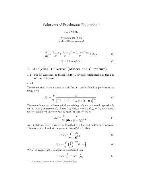
Solutions of Friedmann Equations ∗

Solutions of Friedmann Equations ∗
H 2
H 2 0
= Ωrad,0
a 4
Umut Yildiz
December 20, 2006
Email: yildiz@astro.rug.nl
Ωm,0
+
a3 + 1 − Ωm,0 − ΩΛ,0
a2 + ΩΛ,0
(1)
H0 = 71km/s/Mpc (2)
1 Analytical Universes (Matter and Curvature)
1.1 For an Einstein-de Sitter (EdS) Universe calculatiton of the age
of the Universe.
1.1.1
The cosmic time t as a function of scale factor a can be found by performing the
integral of;
H0t =
a
0
da
Ωr,0
a 2 + Ωm,0
a + ΩΛ,0a 2 + (1 − Ω0)
1/2 . (3)
The fate of a curved universe which containing only matter would depend only
on the density parameter Ω0. Since Ωr,0 = ΩΛ,0 = 0 and Ωm,0 = Ω0 in a curved,
matter dominated universe, the integral (3) turns to be as
H0t =
a
0
da
Ω0
a + (1 − Ω0) . (4)
1/2
An Einstein-de Sitter Universe is described as a flat and matter-only universe.
Therefore Ω0 = 1 and at the present time a(t0) = 1, then
1
H0t0 =
0
1
H0t0 =
0
1
a
da
. (5)
1/2
−1/2 1
da =
a
2
3
With the given Hubble constant in equation 2 then,
H0t0 = 2
3 ⇒ t0 = 2
3H0
∗ Cosmology Lecture, End of Term Computer Task
(6)
(7)

The Hubble constant is given at the value of [km/s/Mpc], then in order to get
the time in terms of Gyr we need to make some conversions like
1 Mpc = 3.085678 × 10 19 km
1 year = 31536000 sec, then
2 × 3.085678 × 10 19 km
3 × 71km/s/Mpc × 31536000s
The age of the EdS universe is 9.187 Gyr.
1.1.2 Computer Calculations
= 9.187Gyr (8)
All the program pieces written for the next tasks calls the module (cosmomodule.py)
given below. It consists of calling some Python modules, constants and
etc...
1.1.3 Python Code
cosmomodule.py
from Numeric import *
from pylab import *
from matplotlib.numerix import *
## Constants
H = 71.0 ## Hubble Constant = 71 km/s/Mpc
Mpc = 3.085677581e+19 #kms
km = 1.0
Gyr= 3.1536e16 #seconds
H0 = (H * Gyr * km / Mpc)
## For LaTeX in the Plots
rc(’text’, usetex=True)
rc(’ps’, usedistiller="xpdf")
## For Legends (Arrays)
openlegend =
[’$\Omega_{0}=1.0$’,’$\Omega_{0}=0.9$’,’$\Omega_{0}=0.8$’,
’$\Omega_{0}=0.3$’,’$\Omega_{0}=0.1$’]
closedlegend =
[’$\Omega_{0}=1.1$’,’$\Omega_{0}=1.2$’,’$\Omega_{0}=1.5$’,
’$\Omega_{0}=2.0$’]
openclosedlegend =
[’$\Omega_{0}=0.1$’,’$\Omega_{0}=0.3$’,’$\Omega_{0}=0.8$’,
’$\Omega_{0}=0.9$’,’$\Omega_{0}=1.0$’,’$\Omega_{0}=1.1$’,
’$\Omega_{0}=1.2$’,’$\Omega_{0}=1.5$’,’$\Omega_{0}=2.0$’]
2

1.2 For EdS Universe plot of a(t) versus t
1.2.1
In Einstein-de Sitter Universe the scale factor as a function of time is found by
t
a(t) =
t0
2/3
where a(t0) is the expansion factor at the present time which is represented by
a circle in the plot.
Figure 1: In EdS Universe, the plot of scale factor a(t) versus time (Gyr)
1.2.2 Python Code
#!/usr/bin/python
#q2.py
from cosmomodule import *
t = arange(0.0,20.0,1)
t0=9.187
a_t = (t/t0)**(2.0/3.0)
plot(t, a_t, ’r’)
scatter(array([t0]), array([1.0]), 20, c=’b’, marker=’o’)
text(9.0,(1.0)**(2.0/3.0)+0.1, "$t = t_{0}$")
title(’${\small Einstein-de Sitter Universe}$’)
xlabel(’t (Gyr)’)
ylabel(’a(t)’)
grid(True)
legend([’$\Omega_{0}=1.0$’])
show()
3
(9)

1.3 For Open Universes with Ω0 = 0.9, 0.8, 0.3, 0.1, present age of
these universes.
1.3.1
In a negatively curved Universe containing only matter (Ω0 < 1, κ = −1), the
present age of the Universe is given by the formula (Ryden [2003], eq 6.44)
1 Ω0
2 − Ω0
H0t0 = −
cosh−1 . (10)
1 − Ω0 2(1 − Ω0) 3/2 Ω0
For the given values of universes with Ω0 = 0.9, 0.8, 0.3, 0.1, present age of these
universes
1.3.2 Python Code
#!/usr/bin/python
#q3.py
from cosmomodule import *
Ω0 t0(Gyr)
0.9 9.3795
0.8 9.5904
0.3 11.1461
0.1 12.3772
def t0(oz): ## oz and omz refers to Omega_{0}
eq=1./(1.-oz) - (oz/(2.*(1.-oz)**(3./2.))* arccosh((2.-oz)/oz))
return eq
omz = array([0.9,0.8,0.3,0.1])
for j in omz:
print t0(j) /(H*Gyr*km/Mpc)
4

1.4 Plot of a(t) versus t for Ω0 = 0.9, 0.8, 0.3, 0.1 Open and Ω0 = 1.0
EdS Universe.
1.4.1 Answer
The analytical solutions of the Friedmann equation for the Open universes is
given in the parametric form in (Ryden [2003], eq 6.20, 6.21). In the equation
the parameter η runs from 0 to infinity.
a(η) = 1
2
Ω0
(cosh η − 1) (11)
1 − Ω0
t(η) = 1 Ω0
(sinh η − η) (12)
2H0 (1 − Ω0) 3/2
Figure 2: Plot of a(t) versus t for Ω0 = 0.9, 0.8, 0.3, 0.1 Open and Ω0 = 1.0 EdS
Universe.
5

1.4.2 Python Code
#!/usr/bin/python
#q4.py
from cosmomodule import *
def aeta(oz, eeta): ## oz and omz refers to Omega_{0}
eq=(1.0/2.0)*(oz/(1.0-oz))*(cosh(eeta)-1.0)
return eq
def teta(oz, eeta):
eq=(1.0/2.0)*(1.0/(H*Gyr*km/Mpc))*(oz/((1.0-oz)**(3.0/2.0)))*(sinh(eeta)-eeta)
return eq
aetaa = []
tetaa = []
eeta = arange(0.0,100.0,0.01)
open= [0.99, 0.90, 0.80, 0.30, 0.1]
agesopen = [9.187, 9.37952716217, 9.5904510966,11.1461044903, 12.3772972365]
for i in range(len(open)):
aetaa.append(aeta(open[i],eeta))
tetaa.append(teta(open[i],eeta))
plot(tetaa[i], aetaa[i])
for i in range(len(agesopen)):
scatter(array([agesopen[i]]), array([1.0]), 20, c=’b’, marker=’o’)
xlim(-0.5,50.0)
ylim(0.0,5.0)
xlabel(’t (Gyr)’)
ylabel(’a(t)’)
legend(openlegend)
grid(True)
show()
6

1.5 For closed universes with Ω0 = 1.1, 1.2, 1.5, 2.0, calculation of the
present age of these Universes
1.5.1
In a positively curved Universe containing only matter (Ω0 > 1, κ = 1), the
present age of the Universe is given by the formula (Ryden [2003], eq 6.43)
Ω0
2 − Ω0
H0t0 =
cos−1
−
2(Ω0 − 1) 3/2 1
(13)
Ω0 − 1
For the given values of universes with Ω0 = 1.1, 1.2, 1.5, 2.0, present age of these
universes
1.5.2 Python Code
#!/usr/bin/python
#q5.py
from cosmomodule import *
Ω0 t0(Gyr)
1.1 9.0111
1.2 8.8483
1.5 8.4238
2.0 7.8662
def t0(oz): ## oz and omz refers to Omega_{0}
eq= ((oz/(2.*(oz-1.)**(3./2.)))*(arccos((2.-oz)/oz)))-(1./(oz-1.))
return eq
omz = [1.1,1.2,1.5,2.0]
for j in omz:
print t0(j)/(H*Gyr*km/Mpc)
7
Ω0

1.6 Calculation of the age of the closed universes at their maximum
size and when they collapse.
1.6.1
The analytical solutions of the Friedmann equation for the Closed Universes is
given in the parametric form in (Ryden [2003], eq 6.17, 6.18). In the equation
the parameter θ runs from 0 to 2π and Big Bang θ = 0 and Big Crunch θ = 2π.
Therefore tmax can be found when the θ = π.
1.6.2 Python Code
#!/usr/bin/python
#q6.py
from cosmomodule import *
thetamax = pi ## For Max Size
thetacrunch = 2.*pi ## For Big Crunch
a(θ) = 1 Ω0
(1 − cos θ) (14)
2 Ω0 − 1
t(θ) = 1 Ω0
(θ − sin θ) (15)
2H0 (Ω0 − 1) 3/2
Ω0 tmax(Gyr) tcollapse(Gyr)
1.1 753.0055 1506.0110
1.2 290.4302 580.8603
1.5 91.8421 183.6842
2.0 43.2948 86.5895
def tmax(oz):
eq=(1./(2.*H))*(oz/((oz-1.)**(3./2.)))*(thetamax-sin(thetamax))
return eq
def tcrunch(oz):
eq=(1./(2.*H))*(oz/((oz-1.)**(3./2.)))*(thetacrunch-sin(thetacrunch))
return eq
omz = [1.1,1.2,1.5,2.0]
for j in omz:
print tmax(j)/(km*Gyr/Mpc)
for j in omz:
print tcrunch(j)/(km*Gyr/Mpc)
8

1.7 Plots of a(t) versus t for the closed universes with Ω0 = 1.1, 1.2, 1.5, 2.0
1.7.1 Plots
Figure 3: Plot of a(t) versus t for the closed universes, Lower plot is the more detailed
of the upper one
9

1.7.2 Python Code
#!/usr/bin/python
#q7.py
from cosmomodule import *
def atheta(oz, thetaa): ## oz refers to Omega_{0}
eq=(1./2.)*(oz/(oz-1.))*(1.-cos(thetaa))
return eq
def ttheta(oz, thetaa):
eq=(1./(2.*H))*(oz/((oz-1.)**(3./2.)))*(thetaa-sin(thetaa))/(km*Gyr/Mpc)
return eq
thetaa = arange(0.0,2.0*pi,0.01)
athetaa = []
tthetaa = []
closed = [1.1, 1.2, 1.5, 2.0]
agesclosed =[9.01115084854, 8.84833006354, 8.4238579855, 7.86623214832]
for i in range(len(closed)):
athetaa.append(atheta(closed[i],thetaa))
tthetaa.append(ttheta(closed[i],thetaa))
plot(tthetaa[i], athetaa[i])
for i in range(len(agesclosed)):
scatter(array([agesclosed[i]]), array([1.0]), 20, c=’b’, marker=’o’)
xlim(-10,1510.0)
ylim(0.0,15.0)
xlabel(’t (Gyr)’)
ylabel(’a(t)’)
legend(closedlegend)
grid(True)
show()
10

1.8 Plots of a(t) versus t and a(t) versus t − t0 for EdS, Overdense
and Underdense Universe Models.
1.8.1 Plots
The combination of the previous plots in one figure. The bottom figure a(t)
versus t − t0 is obtained by subtracting the present age values from the X axis.
Figure 4: Plots of a(t) versus t and a(t) versus t−t0 for EdS, Overdense and Underdense
Universe Models.
11

1.8.2 Python Code
q8x.py
from cosmomodule import *
def aeta(oz, eeta): ## oz and omz refers to Omega_{0}
eq=(1./2.)*(oz/(1.-oz))*(cosh(eeta)-1.)
return eq
def teta(oz, eeta):
eq=(1./2.)*(1./(H*Gyr*km/Mpc))*(oz/((1.-oz)**(3./2.)))*(sinh(eeta)-eeta)
return eq
def atheta(oz, thetaa):
eq=(1./2.)*(oz/(oz-1.))*(1.-cos(thetaa))
return eq
def ttheta(oz, thetaa):
eq=(1./(2.*H))*(oz/((oz-1.)**(3./2.)))*(thetaa-sin(thetaa))/(km*Gyr/Mpc)
return eq
thetaa = arange(0.0,2.0*pi,0.01)
eeta = arange(0.0,100.0,0.01)
aetaa = []
tetaa = []
athetaa = []
tthetaa = []
open= [0.99,0.90,0.80,0.30,0.1]
closed = [1.1, 1.2, 1.5, 2.0]
agesopen = [9.187, 9.3795271621, 9.5904510966,11.1461044903, 12.377297236]
agesclosed =[9.01115084854, 8.84833006354, 8.4238579855, 7.86623214832]
q8a.py
#!/usr/bin/python
#q8a.py (Plot a(t) versus Gyr)
from cosmomodule import *
from q8x import *
for i in range(len(open)):
aetaa.append(aeta(open[i],eeta))
tetaa.append(teta(open[i],eeta))
plot(tetaa[i], aetaa[i])
for i in range(len(closed)):
athetaa.append(atheta(closed[i],thetaa))
tthetaa.append(ttheta(closed[i],thetaa))
plot(tthetaa[i], athetaa[i])
xlim(-0.5,500.0)
ylim(0.0,30.0)
xlabel(’t (Gyr)’)
ylabel(’a(t)’)
legend(openclosedlegend)
grid(True)
show()
q8b.py
#!/usr/bin/python
#q8a.py (Plot a(t) versus t-t0)
from cosmomodule import *
from q8x import *
for i in range(len(open)):
aetaa.append(aeta(open[i],eeta))
tetaa.append(teta(open[i],eeta))
plot(tetaa[i] - agesopen[i], aetaa[i])
for i in range(len(closed)):
athetaa.append(atheta(closed[i],thetaa))
tthetaa.append(ttheta(closed[i],thetaa))
plot(tthetaa[i] - agesclosed[i], athetaa[i])
scatter(array([0.0]), array([1.0]), 20, c=’b’, marker=’o’)
xlim(-20.0,50.0)
ylim(0.0,5.0)
xlabel(’$t - t_{0}$’)
ylabel(’a(t)’)
legend(openclosedlegend,’upper left’)
grid(True)
show()
12

2 Numerical Universes (Matter Radiation Lambda
and Curvature)
In this exercise for different Matter-only Universe models the integration of
H0t =
1
0
Ωm,0
a
da
+ (1 − Ω0)
1/2
(16)
is solved numerically. The calculations of ages for different universe models is
calculated by Mathematica c○ with ‘NIntegrate’ function. And the plot of a(t)
versus t is computed in Matlab.
Here is the comparison of Numerical vs Analytical calculations of t0.
Ω0 Numerical t0(Gyr) Analytical t0(Gyr)
0.1 12.3773 12.37729
0.3 11.1461 11.14610
0.8 9.59045 9.59045
0.9 9.37953 9.37953
1.0 9.18744 9.187
1.1 9.01115 9.01115
1.2 8.84833 8.84833
1.5 8.42386 8.42385
2.0 7.86623 7.86623
It is clearly seen that the analytical solutions and the numerical calculations
of the Friedmann Equation is quite accurate.
2.0.3 Mathematica c○ Code for Present Ages
H = 71.0
Mpc = 3.085677581 ∗ 10 19
km = 1.0
Gyr = 3.1536 ∗ 10 16
H0 = (H ∗ Gyr ∗ km/Mpc)
# Matter-only Universes with different Ω0
1
NIntegrate[
( 1 a − 0.3a2 + 0.3) 1 , {a, 0, 1}]/H0 (17)
2
13

a(t)
1.8
1.6
1.4
1.2
1
0.8
0.6
0.4
0.2
2.0.4 Matlab Code
Numerical Calculations of universe models
0
−5 0 5 10 15 20 25 30
t (Gyr)
Figure 5: Numerical calculated version of Figure 4
Three files are involved in to compute and plot the universe models. In this
computation, I used ‘Trapezoidal Method’ for the numerical approach.
Numerical Approach is defined as
x2
f(x)dx =
x1
x2 − x1
[f(x1) + f(x2)] +
2
(x1 − x2) 3
f”(ξ)
12
error
trapezoidal.m
function y = trapezoidal ( f, a, b, n, oz)
h = (b-a)/n;
x = linspace ( a, b, n+1 );
for i = 1:n+1
fx(i) = universe(x(i),oz );
end
w = [ 0 ones(1,n) ] + [ ones(1,n) 0 ];
if ( nargout == 1 )
y = (h/2) * sum ( w .* fx );
else
disp ( (h/2) * sum ( w .* fx ) );
end
universe.m
function [t]=universe(a,oz)
t = (1.0/((oz/a)+(1.0-oz))^(1/2)) / 0.0725628631386;
plottinguniv.m
a=0:0.01:1.8;
oz = [0.1, 0.3, 0.8, 0.9, 0.9999, 1.1, 1.2, 1.5, 2.0];
for j=1:length(oz),
for i=1:length(a),
univ1(i,j)=trapezoidal(’universe’,0.001,a(i),1000,oz(j));
end
end
plot(univ1,a)
xlabel(’t (Gyr)’)
ylabel(’a(t)’)
14
(18)

2.1 Calculation of the present age of the universe in Concordance,
Loitering, Lambda Collapse, Big Bounce Universes.
2.1.1
Set of Universes:
Concordance Loitering Λ Collapse Big Bounce
Ωm,0 0.27 0.3 1.0 0.3
Ωr,0 4.6 ×10 −5 0.0 0.0 0.0
ΩΛ,0 0.73 1.713 -0.3 1.8
H0t =
a
2.1.2 Mathematica c○ Code
H = 71.0
Mpc = 3.085677581 ∗ 10 1 9
km = 1.0
Gyr = 3.1536 ∗ 10 1 6
H0 = (H ∗ Gyr ∗ km/Mpc)
# Lambda Collapse Universe
Out :8.84375 Gyr
# Concordance
Out :13.6773 Gyr
# Loitering
Out :56.9277 Gyr
# Big Bounce
Out : Error
0
NIntegrate[
da
Ωr,0
a 2 + Ωm,0
a + ΩΛ,0a 2 + (1 − Ω0)
1/2 . (19)
1
NIntegrate[
( 1 a − 0.3a2 + 0.3) 1 , {a, 0, 1}]/H0 (20)
2
( 0.000046
a 2
NIntegrate[
NIntegrate[
1
+ 0.27
a + 0.73a2 − 0.000046) 1 2
1
( 0.3
a + 1.713a2 − 1.013) 1 2
1
( 0.3
a + 1.8a2 − 1.1) 1 2
, {a, 0, 1}]/H0 (21)
, {a, 0, 1}]/H0 (22)
, {a, 0, 1}]/H0 (23)
Since the Big Bounce Universe has no beginning therefore it is not logical to
calculate an age for it.
15

2.2 Calculation of amax for Lambda Collapse Universe
2.2.1
In an Lambda Collapse Universe, the maximum expansion amax is defined as
when the ˙a = 0. Since H = ˙a
a = 0 the Friedmann equation turns to
Ωr,0 Ωm,0
+
a2 a + ΩΛ,0a 2 + (1 − Ω0) = 0 (24)
Then with the given values for Lambda Collapse Universe;
Ωm,0 Ωr,0 ΩΛ,0
Lambda Collapse Universe 1.0 0.0 -0.3
Ω0 = Ωm,0 + Ωr,0 + ΩΛ,0 = 0.7 (25)
0 1
+
a2 a − 0.3a2 + (1 − 0.7) = 0 (26)
1
a − 0.3a2 + 0.3 = 0 (27)
In order to find out the value of a = amin, I used Mathematica c○ . Then, the
result ia found as amax = 1.7155 for Lambda Collapse Universe.
2.2.2 Mathematica c○ Code
Solve[ 1 a − 0.3a2 + 0.3 == 0, a]
2.3 Calculation of amin for Big Bounce Universe
2.3.1
In a Big Bounce Universe, the same definition in the previous exercise applies
and with the given values of Big Bounce Universe Equation 24 becomes as;
Ωm,0 Ωr,0 ΩΛ,0
Big Bounce Universe 0.3 0.0 1.8
Ω0 = Ωm,0 + Ωr,0 + ΩΛ,0 = 2.1 (28)
0 0.3
+
a2 a + 1.8a2 + (1 − 2.1) = 0 (29)
0.3
a + 1.8a2 − 1.1 = 0 (30)
In order to find out the value of a = amin, I used Mathematica c○ Then the
result is found as amin = 0.5598 for Big Bounce Universe.
2.3.2 Mathematica c○ Code
Solve[ 0.3
a + 1.8a2 − 1.1 == 0, a]
16

2.4 Plot of a(t) versus t for Concordance, Loitering, Lambda Collapse
and EdS with Numerical Integration Method.
2.4.1
In order to plot these universes written above I again used Trapozoidal numerical
integration method.
Figure 6: Plot of a(t) versus t for Concordance, Loitering and Lambda Collapse and
EdS
2.4.2 Python Code
#!/usr/bin/python
from numarray import *
from cosmomodule import *
def trapezoid(x, fx):
eq = 0
for i in range(len(x)-1):
eq = eq + (((x[i-1]-x[i])*(fx[i]+fx[i+1]))/2.)
return eq/H0
def universe(a, omegaM, omegaR, omegaL):
omega = omegaM + omegaR + omegaL
uni =1./sqrt( (omegaR/(a**2.)) + omegaM/a + omegaL*(a**2.) + (1.- omega))
return uni
NOSteps = 1000
begin = 1.e-5
end = 5
StepSize = (end - begin) / NOSteps
at = arange(begin, end + StepSize, StepSize)
concordance_time = [0]
concordance_partresult = 0
loitering_time = [0]
loitering_partresult = 0
esd_time = [0]
esd_partresult = 0
lambdacollapse_time = [0]
lambdacollapse_partresult = 0
17

agesmodels =[13.6773, 56.9277, 9.187, 8.84375]
for i in range(1, NOSteps+1):
concordance_y0 = universe(at[i], 0.27, 4.6e-5, 0.73)
concordance_y1 = universe(at[i-1], 0.27, 4.6e-5, 0.73)
concordance_partresult += StepSize * (concordance_y0 + concordance_y1)/2.
concordance_time.append(concordance_partresult / H0)
loitering_y0 = universe(at[i], 0.3, 0., 1.713)
loitering_y1 = universe(at[i-1], 0.3, 0., 1.713)
loitering_partresult += StepSize * (loitering_y0 + loitering_y1)/2.
loitering_time.append(loitering_partresult / H0)
esd_y0 = universe(at[i], 1., 0., 0.)
esd_y1 = universe(at[i-1], 1., 0., 0.)
esd_partresult += StepSize * (esd_y0 + esd_y1)/2.
esd_time.append(esd_partresult / H0)
lambdacollapse_y0 = universe(at[i], 1., 0., -0.3)
lambdacollapse_y1 = universe(at[i-1], 1., 0., -0.3)
lambdacollapse_partresult += StepSize * (lambdacollapse_y0 + lambdacollapse_y1)/2.
lambdacollapse_time.append(lambdacollapse_partresult / H0)
plot(concordance_time, at)
plot(loitering_time, at)
plot(esd_time, at)
plot(lambdacollapse_time, at)
for i in range(len(agesmodels)):
scatter(array([agesmodels[i]]), array([1.0]), 20, c=’b’, marker=’o’)
title(’Universe Models using Trapezoidal Rule’)
xlabel(’t (Gyr)’)
ylabel(’a(t)’)
legend([’Concordance’,’Loitering’,’EdS’,’Lambda Collapse’])
grid(True)
show()
18

2.5 Plot of a(t) versus t − t0 for Concordance, Loitering and Lambda
Collapse, Big Bounce and EdS with Numerical Integration Method.
2.5.1
Figure 7: Plot of a(t) versus t − t0 for Concordance, Loitering and Lambda Collapse
and EdS
2.5.2 Python Code
#!/usr/bin/python
from numarray import *
from cosmomodule import *
def trapezoid(x, fx):
eq = 0
for i in range(len(x)-1):
eq = eq + (((x[i-1]-x[i])*(fx[i]+fx[i+1]))/2.)
return eq/H0
def universe(a, omegaM, omegaR, omegaL):
omega = omegaM + omegaR + omegaL
uni =1./sqrt( (omegaR/(a**2.)) + omegaM/a + omegaL*(a**2.) + (1.- omega))
return uni
NOSteps = 1000
begin = 1.e-5
end = 5
StepSize = (end - begin) / NOSteps
at = arange(begin, end + StepSize, StepSize)
concordance_time = [0]
concordance_partresult = 0
loitering_time = [0]
loitering_partresult = 0
esd_time = [0]
esd_partresult = 0
lambdacollapse_time = [0]
lambdacollapse_partresult = 0
agesmodels =[13.6773, 56.9277, 9.187, 8.84375]
for i in range(1, NOSteps+1):
concordance_y0 = universe(at[i], 0.27, 4.6e-5, 0.73)
19

concordance_y1 = universe(at[i-1], 0.27, 4.6e-5, 0.73)
concordance_partresult += StepSize * (concordance_y0 + concordance_y1)/2.
concordance_time.append((concordance_partresult / H0) - agesmodels[0])
loitering_y0 = universe(at[i], 0.3, 0., 1.713)
loitering_y1 = universe(at[i-1], 0.3, 0., 1.713)
loitering_partresult += StepSize * (loitering_y0 + loitering_y1)/2.
loitering_time.append((loitering_partresult / H0) - agesmodels[1])
esd_y0 = universe(at[i], 1., 0., 0.)
esd_y1 = universe(at[i-1], 1., 0., 0.)
esd_partresult += StepSize * (esd_y0 + esd_y1)/2.
esd_time.append((esd_partresult / H0) - agesmodels[2])
lambdacollapse_y0 = universe(at[i], 1., 0., -0.3)
lambdacollapse_y1 = universe(at[i-1], 1., 0., -0.3)
lambdacollapse_partresult += StepSize * (lambdacollapse_y0 + lambdacollapse_y1)/2.
lambdacollapse_time.append((lambdacollapse_partresult / H0) - agesmodels[3])
plot(concordance_time, at)
plot(loitering_time, at)
plot(esd_time, at)
plot(lambdacollapse_time, at)
scatter(array([0.0]), array([1.0]), 20, c=’b’, marker=’o’)
title(’Universe Models using Trapezoidal Rule’)
xlim(-60,50.0)
ylim(0.0,5.0)
xlabel(’$t - t_{0}$’)
ylabel(’a(t)’)
legend([’Concordance’,’Loitering’,’EdS’,’Lambda Collapse’])
grid(True)
show()
References
B. Ryden. Introduction to cosmology. Introduction to cosmology / Barbara
Ryden. San Francisco, CA, USA: Addison Wesley, ISBN 0-8053-8912-1, 2003,
IX + 244 pp., 2003.
20