SAMPLING VEGETATION ATTRIBUTES - New Mexico NRCS - US ...
SAMPLING VEGETATION ATTRIBUTES - New Mexico NRCS - US ...
SAMPLING VEGETATION ATTRIBUTES - New Mexico NRCS - US ...

Create successful ePaper yourself
Turn your PDF publications into a flip-book with our unique Google optimized e-Paper software.
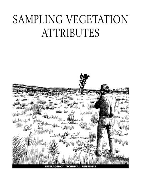
<strong>SAMPLING</strong> <strong>VEGETATION</strong><br />
<strong>ATTRIBUTES</strong><br />
INTERAGENCY TECHNICAL REFERENCE
Sampling Vegetation Attributes<br />
Interagency Technical Reference<br />
Cooperative Extension Service<br />
U.S. Department of Agriculture<br />
— Forest Service —<br />
Natural Resource Conservation Service,<br />
Grazing Land Technology Institute<br />
U.S. Department of the Interior<br />
— Bureau of Land Management —<br />
1996<br />
Revised in 1997, and 1999<br />
Supersedes BLM Technical Reference 4400-4, Trend Studies, dated May 1985<br />
Edited, designed, and produced by the Bureau of Land Management’s<br />
National Applied Resource Sciences Center<br />
BLM/RS/ST-96/002+1730
TABLE OF CONTENTS<br />
<strong>SAMPLING</strong> <strong>VEGETATION</strong> <strong>ATTRIBUTES</strong><br />
Interagency Technical Reference<br />
Bill Coulloudon<br />
Rangeland Management Spec.<br />
Bureau of Land Management<br />
Phoenix, Arizona<br />
Kris Eshelman (deceased)<br />
Rangeland Management Spec.<br />
Bureau of Land Management<br />
Reno, Nevada<br />
James Gianola<br />
Wildhorse and Burro Spec.<br />
Bureau of Land Management<br />
Carson City, Nevada<br />
Ned Habich<br />
Rangeland Management Spec.<br />
Bureau of Land Management<br />
Denver Colorado<br />
Lee Hughes<br />
Ecologist<br />
Bureau of Land Management<br />
St. George, Utah<br />
Curt Johnson<br />
Rangeland Management Spec.<br />
Forest Service Region 4<br />
Ogden Utah<br />
Mike Pellant<br />
Rangeland Ecologist<br />
Bureau of Land Management<br />
Boise, Idaho<br />
By (In alphabetical order)<br />
Technical Reference 1734-4<br />
copies available from<br />
Bureau of Land Management<br />
National Business Center<br />
BC-650B<br />
P.O. Box 25047<br />
Denver, Colorado 80225-0047<br />
Paul Podborny<br />
Wildlife Biologist<br />
Bureau of Land Management<br />
Ely, Nevada<br />
Allen Rasmussen<br />
Rangeland Management Spec.<br />
Cooperative Extension Service<br />
Utah State University<br />
Logan, UT<br />
Ben Robles<br />
Wildlife Biologist<br />
Bureau of Land Management<br />
Safford, Arizona<br />
Pat Shaver<br />
Natural Resource Conservation Service<br />
Rangeland Management Spec.<br />
Corvallis, Oregon<br />
John Spehar<br />
Rangeland Management Spec.<br />
Bureau of Land Management<br />
Rawlins, Wyoming<br />
John Willoughby<br />
State Biologist<br />
Bureau of Land Management<br />
Sacramento, California
TABLE OF CONTENTS<br />
TABLE OF CONTENTS<br />
Page<br />
I. PREFACE ..................................................................................................................i<br />
II. INTRODUCTION ...................................................................................................1<br />
A. Terms and Concepts ...........................................................................................1<br />
B. Techniques Not Addressed ..................................................................................2<br />
C. Guidelines...........................................................................................................3<br />
D. Location of Study Sites .......................................................................................3<br />
E. Key Species ........................................................................................................ 4<br />
F. General Observations..........................................................................................5<br />
G. Coordination .......................................................................................................6<br />
H. Electronic Data Recorders ..................................................................................6<br />
I. Reference Areas ..................................................................................................6<br />
III. STUDY DESIGN AND ANALYSIS..........................................................................7<br />
A. Planning the Study ..............................................................................................8<br />
B. Statistical Considerations ..................................................................................12<br />
C. Other Important Considerations .......................................................................22<br />
IV. <strong>ATTRIBUTES</strong> .........................................................................................................23<br />
A. Frequency .........................................................................................................23<br />
B. Cover ..............................................................................................................25<br />
C. Density .............................................................................................................26<br />
D. Production ........................................................................................................27<br />
E. Structure ...........................................................................................................28<br />
F. Composition .....................................................................................................28<br />
V. METHODS ........................................................................................................... 31<br />
A. Photographs ......................................................................................................31<br />
B. Frequency Methods...........................................................................................37<br />
C. Dry Weight Rank Method .................................................................................50<br />
D. Daubenmire Method ........................................................................................55<br />
E. Line Intercept Method ......................................................................................64<br />
F. Step-Point Method ............................................................................................70<br />
G. Point-Intercept Method ....................................................................................78<br />
H. Cover Board Method ........................................................................................86<br />
I. Density Method ................................................................................................94<br />
J. Double-Weight Sampling................................................................................102<br />
K. Harvest Method ..............................................................................................112<br />
L. Comparative Yield Method .............................................................................116<br />
M. Visual Obstruction Method - Robel Pole ........................................................123<br />
N. Other Methods ...............................................................................................130<br />
VI. GLOSSARY OF TERMS ......................................................................................131<br />
VII. REFERENCES ......................................................................................................139<br />
APPENDIXES ...............................................................................................................149<br />
Appendix A Study Location and Documentation Data Form........................................149<br />
Appendix B Study and Photograph Identification .........................................................153<br />
Appendix C Photo Identification Label .........................................................................157<br />
Appendix D Selecting Random Samples (Using Random Number Tables) ....................161
TABLE OF CONTENTS<br />
TABLE OF CONTENTS (continued)<br />
Illustration Title Page<br />
Number<br />
1 ........ Photo Plot - 3 X 3 Plot Frame Diagram .........................................................34<br />
2 ........ Photo Plot - 5 X 5 Plot Frame Diagram .........................................................35<br />
3 ........ Permanent Photo Plot Location......................................................................36<br />
4 ........ Frequency Form ....................................................................................... 44-45<br />
5 ........ Nested Frequency Form ........................................................................... 46-47<br />
6 ........ Frequency Frame ............................................................................................48<br />
7 ........ Nested Plot Frame..........................................................................................49<br />
8 ........ Dry Weight Rank Form ............................................................................ 53-54<br />
9 ........ Daubenmire Form.................................................................................... 59-60<br />
10 ...... Daubenmire Summary Form ................................................................... 61-62<br />
11 ...... Daubenmire Frame ........................................................................................63<br />
12 ...... Line Intercept Form ................................................................................. 68-69<br />
13 ...... Cover Data Form ..................................................................................... 75-76<br />
14 ...... Sample Units (Hits) and Recording Procedures .............................................77<br />
15 ...... Examples of Sighting Devices ........................................................................83<br />
16 ...... Examples of Pin Frames .................................................................................84<br />
17 ...... Example of a Point Frame ..............................................................................85<br />
18 ...... Cover Board Method: Density Board Form ............................................. 89-90<br />
19 ...... Cover Board Method: Profile Board Form ............................................... 91-92<br />
20 ...... Examples of Cover Boards .............................................................................93<br />
21 ...... Density Form ....................................................................................... 100-101<br />
22 ...... Production Form .................................................................................. 109-110<br />
23 ...... Weight Estimate Quadrat.............................................................................111<br />
24 ...... Comparative Yield Form ...................................................................... 121-122<br />
25 ...... Robel Pole Form................................................................................... 127-128<br />
26 ...... Robel Pole ....................................................................................................129
DEDICATION<br />
DEDICATION<br />
PREFACE<br />
This publication is dedicated to the memory of Kristen R. Eshelman, who<br />
contributed tremendously to its development and preparation. Throughout<br />
his career, Kris was instrumental in producing numerous technical<br />
references outlining procedures for rangeland inventory, monitoring, and<br />
the evaluation of rangeland data. Through his efforts, resource specialists<br />
were provided with the tools to improve the public rangelands for the<br />
benefit of rangeland users and the American public.<br />
i
I. PREFACE<br />
PREFACE<br />
The intent of this interagency monitoring guide is to provide the basis for consistent,<br />
uniform, and standard vegetation attribute sampling that is economical, repeatable,<br />
statistically reliable, and technically adequate. While this guide is not all inclusive, it does<br />
include the primary sampling methods used across the West. An omission of a particular<br />
sampling method does not mean that the method is not valid in specific locations; it simply<br />
means that it is not widely used or recognized throughout the western states. (See Section<br />
V.N, Other Methods.)<br />
Proper use and management of our rangeland resources has created a demand for uniformity<br />
and consistency in rangeland health measurement methods. As a result of this interest, the<br />
<strong>US</strong>DI Bureau of Land Management (BLM) and <strong>US</strong>DA Forest Service met in late 1992 and<br />
agreed to establish an interagency technical team to jointly oversee the development and<br />
publishing of vegetation sampling field guides.<br />
The 13-member team currently includes representatives from the Forest Service, BLM, the<br />
Grazing Land Technology Institute of the Natural Resource Conservation Service (<strong>NRCS</strong>),<br />
and the Cooperative Extension Service.<br />
The interagency technical team first met in January 1994 to evaluate the existing rangeland<br />
monitoring techniques described in BLM’s Trend Studies, Technical Reference TR 4400-4. The<br />
team spent 2 years reviewing, modifying, adding to, and eliminating techniques for this<br />
interagency Sampling Vegetation Attributes technical reference. Feedback from numerous<br />
reviewers, including field personnel, resulted in further refinements.<br />
iii
II. INTRODUCTION<br />
INTRODUCTION<br />
Identifying the appropriate sampling technique first requires the identification of the proper<br />
vegetation characteristic or attribute to measure. To do this the examiner must consider<br />
objectives, life form (grass, forb, shrub, or tree), distribution patterns of individuals of a<br />
species, distribution patterns between species (community mosaic pattern), efficiency of data<br />
collection from an economic standpoint, and accuracy and precision of the data.<br />
Permittees, lessees, other rangeland users, and interested publics should be consulted and<br />
encouraged to participate in the collection and analysis of monitoring data. Those individuals<br />
or groups interested in helping to collect data should be trained in the technique used in the<br />
specific management unit.<br />
This document deals with the collection of vegetation data. The interpretation of that data<br />
will be addressed in other documents. This document does not address interpreting vegetation<br />
data for adjusting livestock numbers or making other management decisions.<br />
A. Terms and Concepts The following terms require an expanded discussion<br />
beyond the scope of the Glossary of Terms:<br />
1. Inventory Inventory is the systematic acquisition and analysis of information<br />
needed to describe, characterize, or quantify vegetation. As might be expected,<br />
data for many different vegetation attributes can be collected. Inventories can be<br />
used not only for mapping and describing ecological sites, but also for determining<br />
ecological status, assessing the distribution and abundance of species, and establishing<br />
baseline data for monitoring studies.<br />
2. Population A population (used here in the statistical, not the biological, sense)<br />
is a complete collection of objects (usually called units) about which one wishes to<br />
make statistical inferences. Population units can be individual plants, points, plots,<br />
quadrats, or transects.<br />
3. Sampling Unit A sampling unit is one of a set of objects in a sample that is<br />
drawn to make inferences about a population of those same objects. A collection<br />
of sampling units is a sample. Sampling units can be individual plants, points,<br />
plots, quadrats, or transects.<br />
4. Sample A sample is a set of units selected from a population used to estimate<br />
something about the population (statisticians call this making inference about the<br />
population). In order to properly make inferences about the population, the units<br />
must be selected using some random procedure (see Technical Reference, Measuring<br />
& Monitoring Plant Populations). The units selected are called sampling units.<br />
5. Sampling Sampling is a means by which inferences about a plant community<br />
can be made based on information from an examination of a small proportion of<br />
that community. The most complete way to determine the characteristics of a<br />
population is to conduct a complete enumeration or census. In a census, each<br />
individual unit in the population is sampled to provide the data for the aggregate.<br />
This process is both time-consuming and costly. It may also result in inaccurate<br />
1
2<br />
INTRODUCTION<br />
values when individual sampling units are difficult to identify. Therefore, the best<br />
way to collect vegetation data is to sample a small subset of the population. If the<br />
population is uniform, sampling can be conducted anywhere in the population.<br />
However, most vegetation populations are not uniform. It is important that data<br />
be collected so that the sample represents the entire population. Sample design is<br />
an important consideration in collecting representative data. (See Section III.)<br />
6. Shrub Characterization Shrub characterization is addressed here since it is<br />
not covered in most of the techniques in this technical reference. Shrub characterization<br />
is the collection of data on the shrub and tree component of a vegetation<br />
community. Attributes that could be important for shrub characterization are<br />
height, volume, foliage density, crown diameter, form class, age class, and total<br />
number of plants by species (density). Another important feature of shrub characterization<br />
is the collection of data on a vertical as well as a horizontal plane.<br />
Canopy layering is also important. The occurrence of individual species and the<br />
extent of canopy cover of each species is recorded in layers. The number of layers<br />
chosen should represent the herbaceous layer, the shrub layer, and the tree layer,<br />
though additional layers can be added if needed.<br />
7. Trend Trend refers to the direction of change. Vegetation data are collected at<br />
different points in time on the same site and the results are then compared to detect<br />
a change. Trend is described as moving “towards meeting objectives,” “away from<br />
meeting objectives,” “not apparent,” or “static.” Trend data are important in determining<br />
the effectiveness of on-the-ground management actions. Trend data indicate<br />
whether the rangeland is moving towards or away from specific objectives. The<br />
trend of a rangeland area may be judged by noting changes in vegetation attributes<br />
such as species composition, density, cover, production, and frequency. Trend data,<br />
along with actual use, authorized use, estimated use, utilization, climate, and other<br />
relevant data, are considered in evaluating activity plans.<br />
8. Vegetation Attributes Vegetation attributes are quantitative features or characteristics<br />
of vegetation that describe how many, how much, or what kind of plant<br />
species are present. The most commonly used attributes are:<br />
Frequency Production<br />
Cover Structure<br />
Density Species Composition<br />
B. Techniques Not Addressed The following are not included in this document:<br />
• Riparian Monitoring<br />
• Monitoring Using Aerial Photography<br />
• Special Status Plant Monitoring<br />
• Weight Estimate and Ocular Reconnaissance Methods<br />
• Soil Vegetation Inventory Method<br />
• Community Structure Analysis Method<br />
• Photo Plot Method
INTRODUCTION<br />
C. Guidelines The techniques described here are guides for establishing and sampling<br />
vegetation attributes. They are not standards. Vegetation sampling techniques and<br />
standards need to be based on management objectives. Techniques can be modified<br />
or adjusted to fit specific resource situations or management objectives as long as the<br />
principles of the technique are maintained. Before a modified technique is used, it<br />
should be reviewed by agency monitoring coordinators, cooperators, and other qualified<br />
individuals. A modified technique should be clearly identified and labeled as<br />
“MODIFIED.” All modifications such as changes in quadrat size or transect layout<br />
should be clearly documented each time the method is used.<br />
D. Location of Study Sites Proper selection of study sites is critical to the<br />
success of a monitoring program. Errors in making these selections can result in<br />
irrelevant data and inappropriate management decisions.<br />
The site selection process used should be documented. Documentation should<br />
include the management objectives, the criteria used for selecting the sites, and the<br />
kinds of comparisons or interpretations expected to be made from them.<br />
Common locations for studies include critical areas and key areas. Some of the site<br />
characteristics and other information that may be considered in the selection of study<br />
sites are:<br />
• Soil<br />
• Vegetation (kinds and distribution of plants)<br />
• Ecological sites<br />
• Seral stage<br />
• Topography<br />
• Location of water, fences, and natural barriers<br />
• Size of pasture<br />
• Kind and/or class of forage animals—livestock, wildlife, wild horses, and wild burros<br />
• Habits of the animals, including foraging<br />
• Areas of animal concentration<br />
• Location and extent of critical areas<br />
• Erosion conditions<br />
• Threatened, endangered, and sensitive species—both plant and animal<br />
• Periods of animal use<br />
• Grazing history<br />
• Location of salt, mineral, and protein supplements<br />
• Location of livestock, wildlife, wild horse, and/or wild burro trails<br />
1. Critical Area Critical areas are areas that should be evaluated separately from<br />
the remainder of a management unit because they contain special or unique<br />
values. Critical areas could include fragile watersheds, sage grouse nesting grounds,<br />
riparian areas, areas of critical environmental concern, etc.<br />
2. Key Areas Key areas are indicator areas that are able to reflect what is happening<br />
on a larger area as a result of on-the-ground management actions. A key area<br />
should be a representative sample of a large stratum, such as a pasture, grazing<br />
allotment, wildlife habitat area, herd management area, watershed area, etc.,<br />
depending on the management objectives being addressed by the study. Key areas<br />
3
4<br />
INTRODUCTION<br />
represent the “pulse” of the rangeland. Proper selection of key areas requires<br />
appropriate stratification. Statistical inference can only be applied to the stratification<br />
unit.<br />
a Selecting Key Areas The most important factors to consider when selecting<br />
key areas are the management objectives found in land use plans, coordinated<br />
resource management plans, and/or activity plans. An interdisciplinary team<br />
should be used to select these areas. In addition, permittees, lessees, and other<br />
interested publics should be invited to participate, as appropriate, in selecting<br />
key areas. Poor information resulting from improper selection of key areas leads<br />
to misguided decisions and improper management.<br />
b Criteria for Selecting Key Areas The following are some criteria that should<br />
be considered in selecting key areas. A key area:<br />
• Should be representative of the stratum in which it is located.<br />
• Should be located within a single ecological site and plant community.<br />
• Should contain the key species where the key species concept is used.<br />
• Should be capable of and likely to show a response to management actions.<br />
This response should be indicative of the response that is occurring on the<br />
stratum.<br />
c Number of Key Areas The number of key areas selected to represent a stratum<br />
ideally depends on the size of the stratum and on data needs. However, the<br />
number of areas may ultimately be limited by funding and personnel constraints.<br />
d Objectives Objectives should be developed so that they are specific to the key<br />
area. Monitoring studies can then be designed to determine if these objectives are<br />
being met.<br />
e Mapping Key Areas Key areas should be accurately delineated on aerial<br />
photos and/or maps. Mapping of key areas will provide a permanent record of<br />
their location.<br />
E. Key Species Key species are generally an important component of a plant<br />
community. Key species serve as indicators of change and may or may not be forage<br />
species. More than one key species may be selected for a stratum, depending on<br />
objectives and data needs. In some cases, problem plants (poisonous, etc.) may be<br />
selected as key species. Key species may change from season to season.<br />
The process used to select key species should be documented. Documentation should<br />
include the management objectives, the criteria used for selecting species, and the kinds<br />
of comparisons or interpretations expected to be made from them.<br />
a Selecting Key Species Selection of key species should be tied directly to<br />
objectives in land-use plans, coordinated resource management plans, and<br />
activity plans. This selection depends upon the plant species in the present<br />
plant community, the present ecological status, and the potential natural communities<br />
for the specific sites. An interdisciplinary team should be used in
INTRODUCTION<br />
selecting key species to ensure that data needs of the various resources are met.<br />
In addition, interested publics should be invited to participate, as appropriate, in<br />
selecting these species (see Section II.G).<br />
b Considerations in Selecting Key Species The following points should be<br />
considered in selecting key species:<br />
• Changes in density, frequency, reproduction, etc., of key species on key areas<br />
are assumed to reflect changes in these species on the entire stratum.<br />
• The forage value of key species may be of secondary or no importance. For<br />
example, watershed protection may require selection of plants as key species<br />
which protect the watershed but are not the best forage species. In some<br />
cases, threatened, endangered, or sensitive species that have no particular<br />
forage value may be selected as key species.<br />
• Any foraging use of the key species on key areas is assumed to reflect foraging<br />
use of that species on the entire stratum.<br />
• Depending on the selected management strategy and/or periods of use, key<br />
species may be foraged during the growing period, after maturity, or both.<br />
• In areas of yearlong grazing use and in areas where there is more than one<br />
use period, several key species may be selected to sample. For example, on<br />
an area with both spring and summer grazing use, a cool season plant may be<br />
the key species during the spring, while a warm season plant may be the key<br />
species during the summer.<br />
• Selection of several key species may be desirable when adjustments in livestock<br />
grazing use are anticipated. This is especially true if more than one plant species<br />
contributes a major portion of the forage base of the animals using the area<br />
(Smith 1965).<br />
c. Key Species on Depleted Rangelands The key species selected should be<br />
present on each key area on which monitoring studies are conducted; however,<br />
on depleted rangelands these species may be sparse or absent. In this situation<br />
it may be necessary to conduct monitoring studies on other species. Data<br />
gathered on non-key species must be interpreted on the basis of effects on the<br />
establishment and subsequent response of the key species. It should also be<br />
verified that the site is ecologically capable of producing the key species.<br />
F. General Observations General observations can be important when conducting<br />
evaluations of grazing allotments, wildlife habitat areas, wild horse and burro<br />
herd management areas, watershed areas, or other designated management areas.<br />
Such factors as rodent use, insect infestations, animal concentrations, fire, vandalism,<br />
and other uses of the sites can have considerable impact on vegetation and soil resources.<br />
This information is recorded on the reverse side of the study method forms or<br />
on separate pages, as necessary.<br />
5
6<br />
INTRODUCTION<br />
G. Coordination Monitoring programs will be coordinated with interested publics<br />
and other appropriate state and federal agencies. Monitoring should be planned and<br />
implemented on an interdisciplinary basis.<br />
H. Electronic Data Recorders Electronic data recorders are handheld “computers”<br />
that are constructed to withstand the harsh environmental conditions found in<br />
the field. They are used to record monitoring data in a digital format that can be<br />
transferred directly to a personal computer for storage and retrieval. They require<br />
minimal maintenance, are generally programmable, and allow easy data entry using a<br />
wand and bar codes.<br />
Recording field data using an electronic data recorder takes approximately the same<br />
amount of time as using printed forms. The advantage with electronic data recorders<br />
is that they improve the efficiency by reducing errors associated with entering data<br />
into a computer for analysis. They can also reduce the time needed for data compilation<br />
and summarization.<br />
The cost of electronic data recorders and computer software programs is considerable<br />
and should be evaluated prior to purchase. It is also important to have good computer<br />
support assistance available to assist users in operating, downloading, and troubleshooting<br />
electronic data recorders, especially during the initial use period.<br />
I. Reference Areas Reference areas are rangelands where natural biological and<br />
physical processes are functioning normally. Reference areas serve as benchmarks for<br />
comparing management actions on rangelands. Reference areas differ from key areas<br />
in that they represents rangeland where impacts are minimal. Reference areas are<br />
found in grazing exclosures, natural areas, or areas that receive minimal grazing impacts.<br />
Reference areas should be included in any monitoring program to evaluate the influences<br />
of natural variables (especially climate) on vegetation. Cause-and-effect relationships<br />
are better determined if the effects of climate on vegetation can be separated<br />
from management effects. Monitoring studies, especially trend studies, should therefore<br />
be established both on key areas and reference areas located on the same ecological<br />
sites. Of course, monitoring priorities and funding resources must be considered in<br />
planning and establishing monitoring studies on reference areas.
STUDY DESIGN AND ANALYSIS<br />
III. STUDY DESIGN AND ANALYSIS<br />
The rangeland monitoring methods described in Section V have a number of common<br />
elements. Those that relate to permanently marking and documenting the study location<br />
are described in detail below.<br />
Also discussed in this section are statistical considerations (target populations, random<br />
sampling, systematic sampling, confidence intervals, etc.) and other important factors (properly<br />
identifying plant species and training people so they follow the correct procedures).<br />
It is important to read this chapter before referring to the specific methods described in<br />
Section V, since the material covered here will not be repeated for each of them.<br />
Permanently Marking the Study Location Permanently mark the location of each study<br />
by means of a reference post (steel post) placed about 100 feet from the actual study<br />
location. Record the bearing and distance from the post to the study location. An alternative<br />
is to select a reference point, such as a prominent natural or man-made feature, and<br />
record the bearing and distance from that point to the study location. If a post is used, it<br />
should be tagged to indicate that it marks the location of a monitoring study and should<br />
not be disturbed.<br />
Permanently mark the study location itself by driving angle iron stakes into the ground at<br />
randomly selected starting points. The baseline technique requires that both ends of the<br />
baseline be permanently staked. With the macroplot technique, a minimum of three<br />
corners need to be permanently staked. If the linear technique is used, only the beginning<br />
point of the study needs to be permanently staked. Establish the study according to the<br />
directions found in Section III.A.2 beginning on page 8.<br />
Paint the transect location stake with brightly colored permanent spray paint (yellow or<br />
orange) to aid in relocation. Repaint this stake when subsequent readings are made.<br />
Study Documentation Document the study and transect locations, number of transects,<br />
starting points, bearings, length, distance between transects, number of quadrats, sampling<br />
interval, quadrat frame size, size of plots in a nested plot frame technique, number of<br />
cover points per quadrat frame, and other pertinent information concerning a study on the<br />
Study Location and Documentation Data form (see Appendix A). For studies that use a<br />
baseline technique, record the location of each transect along the baseline and the direction<br />
(left or right).<br />
Be sure to document the exact location of the study site and the directions for relocating<br />
it. For example: 1.2 miles from the allotment boundary fence on the Old County Line Road.<br />
The reference post is on the south side of the road, 50 feet from the road.<br />
Plot the precise location of the study on detailed maps and/or aerial photos.<br />
7
8<br />
STUDY DESIGN AND ANALYSIS<br />
A. Planning the Study Proper planning is by far the most important part of a<br />
monitoring study. Much wasted time and effort can be avoided by proper planning.<br />
A few important considerations are discussed below. The reader should refer to<br />
Technical Reference, Measuring & Monitoring Plant Populations, for a more complete<br />
discussion of these important steps.<br />
1. Identify Objectives Based on land use and activity plans, identify objectives<br />
appropriate for the area to be monitored. The intent is to evaluate the effects of<br />
management actions on achieving objectives by sampling specific vegetation<br />
attributes.<br />
2. Design the Study The number of quadrats, points, or transects (sample size)<br />
needed depends on the objectives and the efficiency of the sampling design. It should<br />
be known before beginning the study how the data will be analyzed. The frequency of<br />
data collection (e.g., every year, every other year, etc.) and data sheet design should be<br />
determined before studies are implemented. The sample data sheets included with<br />
each method (following the narrative) are only examples of data forms. Field<br />
offices have the option to modify these forms or develop their own.<br />
All of the methods described in this document can be established using the following<br />
techniques:<br />
a Baseline A baseline is established by stretching a tape measure of any desired<br />
length between two stakes (figure 1). For an extremely long baseline, intermediate<br />
stakes can be used to ensure proper alignment. It is recommended that<br />
metric measurement be used. Individual transects are then run perpendicular to<br />
the baseline at random locations along the tape. The location of quadrats along<br />
these transects can be either measured or paced. Transects can all be run in the<br />
same direction, in which case the baseline forms one of the outer boundaries of<br />
the sampled area, or in two directions, in which case the baseline runs through<br />
the center of the sampled area. If transects are run in two directions, the direction<br />
for each individual transect should be determined randomly. (Directions<br />
for randomly selecting the location of transects to be run off of a baseline using<br />
a random numbers table are given in Appendix D). Quadrats or observation<br />
points are spaced at specified distances along the transect. This study design is<br />
intended to randomly sample a specified area. The area to be sampled can be<br />
expanded as necessary by lengthening the baseline and/or increasing the length<br />
between quadrats or sampling points.<br />
This design may need to be modified for riparian areas or other areas where the<br />
area to be sampled is long and narrow. For these areas, a single linear transect<br />
may be more appropriate.<br />
b Macroplot The concept with this type of design is to allow every area within<br />
the study site or sample area to have an equal chance to be sampled. A<br />
macroplot is a large square or rectangular study site. The size of the macroplot<br />
will depend on the size of the study site. The macroplot should encompass<br />
most of the study site. From the standpoint of statistical inference, it is best,<br />
once the macroplot boundaries have been determined, to redefine the study site<br />
to equal the macroplot. Examples of macroplot sizes are 50 m x 100 m, 100 m<br />
x 100 m, and 100 m x 200 m, but much larger macroplots can be used to cover<br />
larger study sites. Macroplot size and shape should be tailored to each situation.
Photo plots may be<br />
permanently located<br />
anywhere along the<br />
baseline tape.<br />
Baseline End Point Stake<br />
Transect 3<br />
Transect 2<br />
Baseline Beginning Point Stake<br />
∆<br />
∆<br />
∆<br />
STUDY DESIGN AND ANALYSIS<br />
Study Layout<br />
100-Meter Baseline Tape<br />
∆<br />
Figure 1. Study layout for the baseline technique.<br />
Transect 1<br />
Study Location Stake<br />
9
10<br />
STUDY DESIGN AND ANALYSIS<br />
Macroplot size also depends on the size and shape of the quadrats that will be<br />
used to sample it. The sides of the macroplot should be of dimensions that are<br />
multiples of the sides of the quadrats.<br />
(1) Macroplot layout Pick one corner of the macroplot to serve as the beginning<br />
for sampling purposes. Drive an angle iron location stake into the ground<br />
at this corner. Determine the bearing of the macroplot side that will serve<br />
as the x-axis, run a tape in that direction and put an angle iron stake at the<br />
selected distance. This serves as another corner of the macroplot. Leave<br />
the x-axis tape in place for sampling purposes. Return to the origin and<br />
determine the bearing of the y-axis, which will be perpendicular to the xaxis.<br />
Run a second tape along the y-axis and put an angle iron stake in the<br />
ground at the selected distance. This serves as the third corner of the<br />
macroplot. If desired, a fourth stake may be placed at the remaining<br />
corner, but this is not necessary for sampling since sampling will be done<br />
using the two tapes serving as the x- and y-axes. See Figure 2 for an example.<br />
Leave the tapes in place until the first year’s sampling is completed.<br />
50 m<br />
angle iron<br />
0 m<br />
0 m 100 m<br />
Figure 2. The two sides of a 50 m x 100 m macroplot, delineated by two tape measures. Both tapes begin<br />
with their 0 point at the beginning. Note placement of angle irons at three of the corners.<br />
Be sure to document the directions of the x- and y-axes so that the<br />
macroplot can be reconstructed if one of the angle iron stakes is missing.<br />
(2) Quadrat locations Quadrats are located in the macroplot using a coordinate<br />
system to identify the lower left-hand corner of each quadrat.<br />
(a) For example it has been determined from the pilot study that 40<br />
samples are needed using a 1 m by 16 m quadrat. The quadrats are to<br />
be positioned so that the long side is parallel to the x-axis. On a 40 m<br />
x 80 m study site (see Figure 3), the x-axis would be the 80 m side.<br />
The total number of quadrats (N) that could be placed in that 40 m x<br />
80 m rectangle without overlap comprises the sampled population. In<br />
this case, N is equal to 200 quadrats.<br />
(b) Along the x-axis there are 5 possible starting points (which always occur<br />
at the lower left-hand corner of each quadrat) for each 1 m x 16 m<br />
quadrat (at points 0 m, 16 m, 32 m, 48 m, and 64 m). Number these<br />
points 0 to 4 (in whole numbers) accordingly. Along the y-axis there are<br />
40 possible starting points for each quadrat (at points 0 m, 1 m, 2 m, 3 m,<br />
4 m, and so on until point 39 m). Number these points 0 to 39 accordingly<br />
(again in whole numbers)
39<br />
30<br />
20<br />
10<br />
Y<br />
axis<br />
STUDY DESIGN AND ANALYSIS<br />
16m 32m 48m 64m 80m<br />
0<br />
0 1<br />
2 3 4 5<br />
Beginning Point Stake<br />
Figure 3. A 40 m x 80 m macroplot showing the 200 possible quadrats of size 1 m x 16 m that could be<br />
placed within it (assuming the long side of the quadrats is oriented along the x-axis).<br />
(c) Now, using a random number table or a random number generator on<br />
a computer or handheld calculator, choose at random 40 numbers<br />
from 0 to 4 for the x axis and 40 numbers from 0 to 39 for the y axis.<br />
(Directions on the use of random number tables and random number<br />
generators are given in Appendix D of this document and in Technical<br />
Reference, Measuring & Monitoring Plant Populations.<br />
(d) At the end of this process, 40 pairs of coordinates will be selected. If<br />
any pair of coordinates is repeated, the second pair is rejected and<br />
another pair picked at random to replace it (because sampling is<br />
without replacement). Continue until there are 40 unique pairs of<br />
coordinates.<br />
These 40 pairs of coordinates mark the points at which quadrats will<br />
be positioned.<br />
(e) Both to increase sampling efficiency and to reduce impacts to the<br />
sampling units by examiners, the coordinates should be ordered from<br />
smallest to largest first on the axis parallel to the longest side of the<br />
quadrat and then on the other axis. For example, the following four<br />
sets of coordinates have been randomly selected (presented in the<br />
order they were selected):<br />
x-axis y-axis<br />
1. 3 (48.0 m) 27.0 m<br />
2. 4 (64.0 m) 34.0 m<br />
3. 3 (48.0 m) 8.0 m<br />
4. 1 (16.0 m) 28.0 m<br />
X<br />
axis<br />
11
12<br />
STUDY DESIGN AND ANALYSIS<br />
Because the quadrats are being placed with their long side parallel to<br />
the x-axis, the coordinates are ordered first by the x-axis and next by<br />
the y-axis. Thus the new order is as follows:<br />
x-axis y-axis<br />
1. 16.0 m 28.0 m<br />
2. 48.0 m 8.0 m<br />
3. 48.0 m 27.0 m<br />
4. 64.0 m 34.0 m<br />
In each column defined by an x-coordinate, sampling starts from the<br />
bottom of the macroplot and moves to the top. This systematic<br />
approach ensures that quadrats are not walked on until after they have<br />
been read.<br />
c Linear This study design samples a study site in a straight line. Because it<br />
samples such a small segment of the sample area, this technique is not<br />
recommended except for long, narrow study sites such as riparian areas.<br />
Randomly select the beginning point of the transect within the study site and<br />
mark it with a stake to permanently locate the transect (figure 4). Randomly<br />
determine the transect bearing and select a prominent distant landmark such as<br />
a peak, rocky point, etc., that can be used as the transect bearing point. Vegetation<br />
attribute readings are taken at a specified interval (paced or measured)<br />
along the transect bearing. If the examiner is unable to collect an adequate<br />
sample with this transect before leaving the study site, additional transects can<br />
be run from the transect location stake at different bearings.<br />
B. Statistical Considerations<br />
1. Target Population Study sites are selected (subjectively) that hopefully reflect<br />
what is happening on a larger area. These may be areas that are considered to be<br />
representative of a larger area such as a pasture (see Section II.D.2 for more discussion<br />
of key areas) or critical areas such as sites where endangered species occur.<br />
Monitoring studies are then located in these areas. Since these study sites are<br />
subjectively selected, no valid statistical projections to an entire allotment are<br />
possible. Therefore, careful consideration and good professional judgement must<br />
be used in selecting these sites to ensure the validity of any conclusions reached.<br />
a Although it would be convenient to make inferences from sampling study sites<br />
regarding the larger areas they are chosen to represent, there is no way this can be<br />
done in the statistical sense because the study sites have been chosen subjectively.<br />
b For this reason it is important to develop objectives that are specific to these<br />
study sites. It is equally important to make it clear what actions will be taken<br />
based on what happens on the study sites.<br />
c It is also important to base objectives and management actions on each study site<br />
separately. Values from study sites from different strata should never be averaged.
End Point of Transect<br />
100-Meter Tape<br />
Midpoint of Transect<br />
Beginning Point of Transect<br />
Figure 4. Study layout for the linear technique.<br />
STUDY DESIGN AND ANALYSIS<br />
Transect Bearing Stake<br />
Quadrats<br />
Study Location Stake<br />
13
14<br />
STUDY DESIGN AND ANALYSIS<br />
d From a sampling perspective, it is the study site that constitutes the target<br />
population. The collection of all possible sampling units that could be placed in<br />
the study site is the target population.<br />
2. Random Sampling Critical to valid monitoring study design is that the sample<br />
be drawn randomly from the population of interest. There are several methods of<br />
random sampling, many of which are discussed briefly below, but the important<br />
point is that all of the statistical analysis techniques available are based on knowing<br />
the probability of selecting a particular sampling unit. If some type of random<br />
selection of sampling units is not incorporated into the study design, the probability<br />
of selection cannot be determined and no statistical inferences can be made<br />
about the population. (Directions for randomly selecting the location of transects<br />
to be run off of a baseline using random number tables are given in Appendix D).<br />
3. Systematic Sampling Systematic sampling is very common in sampling<br />
vegetation. The placement of quadrats along a transect is an example of systematic<br />
sampling. To illustrate, let’s say we decide to place ten 1-square-meter quadrats at<br />
5-meter (or 5-pace) intervals along a 50-meter transect. We randomly select a<br />
number between 0 and 4 to represent the starting point for the first quadrat along<br />
the transect and place the remaining 9 quadrats at 5-meter intervals from this<br />
starting point. Thus, if 10 observations are to be made at 5-meter intervals and the<br />
randomly selected number between 0 and 4 is 2, then the first observation is made<br />
at 2 meters and the remaining observations will be placed at 7, 12, 17, 22, 27, 32,<br />
37, 42, and 47 meters along the transect. The selection of the starting point for<br />
systematic sampling must be random.<br />
Strictly speaking, systematic sampling is analogous to simple random sampling only<br />
when the population being sampled is in random order (for example, see Williams<br />
1978). Many natural populations exhibit an aggregated (also called clumped)<br />
spatial distribution pattern. This means that nearby units tend to be similar to<br />
(correlated with) each other. If, in a systematic sample, the sampling units are<br />
spaced far enough apart to reduce this correlation, the systematic sample will tend<br />
to furnish a better average and smaller standard error than is the case with a<br />
random sample, because with a completely random sample one is more likely to<br />
end up with at least some sampling units close together (see Milne 1959 and the<br />
discussion of sampling an ordered population in Scheaffer et al. 1979).<br />
4. Sampling vs. Nonsampling Errors In any monitoring study, it pays to keep<br />
the error rate as low as possible. Errors can be separated into sampling errors and<br />
nonsampling errors.<br />
a Sampling Errors Sampling errors arise from chance variation; they do not<br />
result from “mistakes” such as misidentifying a species. They occur when the<br />
sample does not reflect the true population. The magnitude of sampling errors<br />
can be measured.<br />
b Nonsampling Errors Nonsampling errors are “mistakes” that cannot be measured.
Examples of nonsampling errors include the following:<br />
STUDY DESIGN AND ANALYSIS<br />
• Using biased selection rules, such as selecting “representative samples” by<br />
subjectively locating sampling units or substituting sampling units that are<br />
“easier” to measure.<br />
• Using sampling units in which it is impossible to accurately count or estimate<br />
the attribute in question.<br />
• Sloppy field work.<br />
• Transcription and recording errors.<br />
• Incorrect or inconsistent species identification.<br />
To minimize nonsampling errors:<br />
• Design studies to minimize nonsampling errors. For example, if canopy cover<br />
estimates are needed, point intercept or line intercept techniques result in<br />
smaller nonsampling errors than the use of quadrats (Floyd and Anderson<br />
1987; Kennedy and Addison 1987; Buckner 1985). For density data, select a<br />
quadrat size that doesn’t contain too many individual plants, stems, etc., to<br />
count accurately.<br />
• When different personnel are used, conduct rigorous training and testing to<br />
ensure consistency in measurement and estimation.<br />
• Design field forms that are easy to use and not confusing to data transcribers.<br />
Double (or triple) check all data entered into computer programs to ensure<br />
the numbers are correct.<br />
5. Confidence Interval In rangeland monitoring, the true population total (or any<br />
other true population parameter) will never be known. The best way to judge how<br />
well a sample estimates the true population total is by calculating a confidence interval.<br />
The confidence interval is a range of values that is expected to include the true population<br />
size (or any other parameter of interest, often an average) a given percentage<br />
of the time (Krebs 1989). For instructions in calculating confidence intervals, see<br />
Technical Reference, Measuring & Monitoring Plant Populations.<br />
6. Quadrat Size and Shape Quadrat size and shape can have a major influence<br />
on the precision of the estimate.<br />
a Frequency Frequency is most typically measured in square quadrats. Because<br />
only presence or absence is measured, square quadrats are fine for this purpose.<br />
Of most concern in frequency measurement is the size of the quadrat. Good<br />
sensitivity to change is obtained for frequency values between 20 percent and<br />
80 percent (Despain et al. 1991). Frequency values between 10 percent and 90<br />
percent are still useful, but values outside this range should be used only to<br />
indicate species presence, not to detect change (Despain et al. 1991). Because<br />
frequency values are measured separately for each species, what constitutes an<br />
optimum size quadrat for one species may be less than optimum or even inappropriate<br />
for another. This problem is partially resolved by using nested plot quadrats<br />
of different sizes (refer to Frequency Method, Section V.B).<br />
15
16<br />
STUDY DESIGN AND ANALYSIS<br />
b Cover In general, quadrats are not recommended for estimating cover (Floyd<br />
and Anderson 1987; Kennedy and Addison 1987). Where they are used, the<br />
same types of considerations given below for density apply: long, thin quadrats<br />
will likely be better than circular, square, or shorter and wider rectangular<br />
quadrats (Krebs 1989). Each situation, however, should be analyzed separately.<br />
The amount of area in the quadrat is a concern with cover estimation. The<br />
larger the area, the more difficult it is to accurately estimate cover.<br />
c Density Long, thin quadrats are better (often very much better) than circles,<br />
squares, or shorter and wider quadrats. How narrow the quadrats can be depends<br />
upon consideration of problems of edge effect, although problems of edge<br />
effect can be largely eliminated by developing consistent rules for determining<br />
whether to include or exclude plants that fall directly under quadrat edges.<br />
One recommendation is to count plants that are rooted directly under the top<br />
and left sides of the quadrat but not those directly rooted under the bottom and<br />
right quadrat sides. The amount of area within the quadrat is limited by the<br />
degree of accuracy with which one can count all the plants within each quadrat.<br />
d Plant Biomass For the same reason as given for density, long, thin quadrats are<br />
likely to be better than circular, square, or shorter and wider rectangular quadrats<br />
(Krebs 1989). Edge effect can result in significant measurement bias if the<br />
quadrats are too small (Wiegert 1962). Since above-ground vegetation must be<br />
clipped in some quadrats, circular quadrats should be avoided because of the<br />
difficulty in cutting around the perimeter of the circle with hand shears and the<br />
likely measurement bias that would result. If plant biomass is collected in<br />
grams, it can be easily converted to pounds per acres if the total area sampled is<br />
a multiple of 9.6 ft 2 .<br />
Use the following table to convert grams to pounds per acre:<br />
Table 1<br />
(# of plots x size = total area)<br />
(10 x 0.96 = 9.6 ft2 ) multiply grams times 100 = pounds per acre<br />
(10 x 1.92 = 19.2 ft2 ) multiply grams times 50 = pounds per acre<br />
(10 x 2.40 = 24.0 ft2 ) multiply grams times 40 = pounds per acre<br />
(10 x 4.80 = 48.0 ft2 ) multiply grams times 20 = pounds per acre<br />
(10 x 9.60 = 96.0 ft2 ) multiply grams times 10 = pounds per acre<br />
(10 x 96.0 = 960.0 ft2 ) multiply grams times 1 = pounds per acre<br />
7. Interspersion One of the most important considerations of sampling is good<br />
interspersion of sampling units throughout the area to be sampled (the target<br />
population).<br />
The basic goal should be to have sampling units as well interspersed as possible<br />
throughout the area of the target population. The practice of placing all of the<br />
sampling units, whether they be quadrats or points, along a single transect or even<br />
a few transects should be avoided, because it results in poor interspersion of<br />
sampling units and makes it unlikely that the sample will provide a representative<br />
sample of the target population. This is true even if the transect(s) is randomly<br />
located.<br />
8. Pilot Studies The purposes of pilot studies are to select the optimum size and/
STUDY DESIGN AND ANALYSIS<br />
or shape of the sampling unit for the study and to determine how much variability<br />
exists in the population being sampled. The latter information is necessary to<br />
determine the sample size necessary to meet specific management and monitoring<br />
objectives.<br />
a Initial Considerations Before beginning the actual pilot study, subjectively<br />
experiment with different sizes and shapes of sampling units. For example, if<br />
estimating density, subjectively place quadrats 1 of a certain size and shape in<br />
areas with large numbers of the target plant species. Then see how many plants<br />
fall into the quadrat and ascertain if this is too many to count. See what kind of<br />
problems there might be with edge effect: when individuals fall on or near one<br />
of the long edges of the quadrat, will it be difficult for examiners to make<br />
consistent calls as to whether these individuals are in or out of the quadrat? 2<br />
See if there is a tendency to get more plants in rectangular quadrats when they<br />
are run one way as opposed to another. If so, then the quadrats should be run in<br />
the direction that hits the most plants. Otherwise it is likely that some quadrats<br />
will have few to no plants in them, while others will have many; this is highly<br />
undesirable. The goal should be to end up with similar numbers of plants in<br />
each of the quadrats, while still sampling at random.<br />
If transects or lines are the sampling units, subjectively lay out lines of different<br />
lengths and in different directions. See if the lines cross most of the variability<br />
likely to be encountered with respect to the target plant species. If not, they<br />
may need to be longer. Don’t make the lines so long, however, that it will be<br />
difficult to measure them, especially if there are a lot of lines involved. As with<br />
rectangular quadrats, it is desirable to have each of the lines encountering<br />
similar numbers and/or cover values of the target species, while still sampling at<br />
random.<br />
b Efficiency of Sample Design Pilot sampling allows the examiner to compare<br />
the efficiency of various sampling designs. By dividing the sample standard<br />
deviation by the sample average, the coefficient of variation is obtained.<br />
Comparing coefficients of variation allows one to determine which of two or<br />
more sampling designs is most efficient (the lower the coefficient of variation,<br />
the greater the efficiency of the sampling design).<br />
Conduct a pilot study by randomly positioning a number of sampling units of<br />
different sizes and shapes within the area to be sampled and then choosing the<br />
size and shape that yields the smallest coefficient of variation.<br />
The following shows how to calculate the standard deviation for the density of<br />
1 Note that it is not necessary to construct an actual frame for the quadrats used. It is sufficient to delineate<br />
quadrats using a combination of tape measures and meter (or yard) sticks. For example, a 5 m x 0.25 m<br />
quadrat can be constructed by selecting a 5 m interval along a meter tape, placing two 1-meter sticks perpendicular<br />
to the tape at both ends of the interval (with their zero points at the tape), and laying another tape or<br />
rope across these two sticks at their 0.25 m points. This then circumscribes a quadrat of the desired size and<br />
shape.<br />
2 Often, problems with edge effect can be largely overcome by making a rule that any plants that fall on the left<br />
or top edges of the quadrat are counted, whereas any plants that fall on the right or bottom edges of the<br />
quadrat are not counted.<br />
17
18<br />
STUDY DESIGN AND ANALYSIS<br />
sideoats grama occurring in two sample designs. In this example there are 2, 10,<br />
and 21 sideoats grama plants in three separate quadrats in the first design and 9,<br />
10, and 14 sideoats grama plants in the second set of three plots. The average<br />
number of plants in both sets of plots is 11 (2+10+21= 33/3= 11 and 9+10+14=<br />
33/3=11). The standard deviation is calculated as follows:<br />
(X1 - X)<br />
where:<br />
S = standard deviation<br />
X = number of plants<br />
X = the mean or average number of plants per quadrat<br />
n = the number of samples (quadrats in this example)<br />
2 + (X2 - X) 2 + . . . + (Xn - X) 2 (X - X) 2<br />
S = or S =<br />
n -1<br />
n -1<br />
Number of plants<br />
2<br />
10<br />
21<br />
Deviation<br />
(X - X)<br />
2 - 11 = -9<br />
10 - 11 = -1<br />
21 - 11 = 10<br />
Squared<br />
Deviation<br />
(X - X)<br />
81<br />
1<br />
100<br />
2<br />
X = 33/3 = 11 182<br />
(X - X) 2 182 182<br />
S = = = = 91 = 9.54<br />
n -1 3 -1 2<br />
Number of plants<br />
9<br />
10<br />
14<br />
Deviation<br />
(X - X)<br />
9 - 11 = -2<br />
10 - 11 = -1<br />
14 - 11 = 3<br />
Squared<br />
Deviation<br />
(X - X)<br />
4<br />
1<br />
9<br />
2<br />
X = 33/3 = 11 14<br />
(X - X) 2 14 14<br />
S = = = = 7 = 2.65<br />
n -1 3 -1 2<br />
The coefficient of variation for the first set of quadrats is 9.54/11 or .86,<br />
whereas the second set of quadrats has a coefficient of variation of 2.65/11= .24.<br />
Since the second sampling design has the lowest coefficient of variation, it is the<br />
most efficient design.<br />
This example, with only three quadrats in each sampling design, is given solely to show how<br />
to calculate standard deviations and coefficients of variation. When comparing actual<br />
study designs, ensure that the sample standard deviation is a good estimate of the population<br />
standard deviation. One way of ensuring this is to construct sequential sampling<br />
graphs of the standard deviation of each design (see Sequential Sampling below).
STUDY DESIGN AND ANALYSIS<br />
Wiegert (1962), summarized in Krebs (1989:67-72), gives a quantitative<br />
method for determining optimal quadrat size and/or shape. The method considers<br />
the costs involved in locating and measuring quadrats and the standard<br />
deviation (or its square, the variance) that results from samples of that size and<br />
shape. Refer to Krebs’ book for details (and an example).<br />
c Sequential Sampling The estimate of the standard deviation derived through<br />
pilot sampling is one of the values used to calculate sample size, whether one<br />
uses the formulas given in Technical Reference, Measuring & Monitoring Plant<br />
Populations, or uses a computer program.<br />
When conducting the pilot sampling, employ sequential sampling. Sequential<br />
sampling helps determine whether the examiner has taken a large enough pilot<br />
sample to properly evaluate different sampling designs and/or to use the standard<br />
deviation from the pilot sample to calculate sample size. The process is<br />
accomplished as follows:<br />
Gather pilot sampling data using some arbitrarily selected sample size. Calculate<br />
the average and standard deviation for the first two quadrats, calculate it again<br />
after putting in the next quadrat value, and continue these iterative calculations<br />
after the addition of each quadrat value to the sample. This will generate a<br />
running average and standard deviation. Look at the four columns of numbers on<br />
the right of Figure 5 for an example of how to carry out this procedure.<br />
Plot on graph paper (or use a computer program) the sample size versus the<br />
average and standard deviation. Look for curves smoothing out. In the example<br />
shown in Figure 5, the curves smooth out after n = 30-35. The decision to stop<br />
sampling is a subjective one. There are no hard and fast rules.<br />
A computer is valuable for creating sequential sampling graphs. Spreadsheet<br />
programs such as Lotus 1-2-3 allow for entering the data in a form that can later<br />
be analyzed while at the same time creating a sequential sampling graph of the<br />
running average and standard deviation. This further allows the examiner to<br />
look at several random sequences of the data before deciding on the number of<br />
sampling units to measure.<br />
Use the sequential sampling method to determine what sample size not to use<br />
(don’t use a sample size below the point where the running average and<br />
standard deviation have not stabilized). Plug the final average and standard<br />
deviation information into the appropriate sample size equation to actually<br />
determine the necessary sample size.<br />
19
4<br />
3.5<br />
3<br />
2.5<br />
20<br />
5<br />
STUDY DESIGN AND ANALYSIS<br />
10<br />
Example of a sequential sampling graph<br />
15<br />
20<br />
25 30<br />
Sample size<br />
Figure 5. Example of a sequential sampling graph. The running average and standard deviation are plotted<br />
for sample sizes of n=5 up to n=50. Sampling was conducted in an area of 50 m x 100 m with a quadrat size<br />
of 1 m x 5 m. Actual values are shown on the right.<br />
35<br />
40<br />
Average<br />
45<br />
SD<br />
50<br />
N<br />
1<br />
2<br />
3<br />
4<br />
5<br />
6<br />
7<br />
8<br />
9<br />
10<br />
11<br />
12<br />
13<br />
14<br />
15<br />
16<br />
17<br />
18<br />
19<br />
20<br />
21<br />
22<br />
23<br />
24<br />
25<br />
26<br />
27<br />
28<br />
29<br />
30<br />
31<br />
32<br />
33<br />
34<br />
35<br />
36<br />
37<br />
38<br />
39<br />
40<br />
41<br />
42<br />
43<br />
44<br />
45<br />
46<br />
47<br />
48<br />
49<br />
50<br />
Plants<br />
1<br />
2<br />
0<br />
9<br />
5<br />
7<br />
1<br />
0<br />
8<br />
1<br />
0<br />
0<br />
4<br />
4<br />
2<br />
0<br />
4<br />
0<br />
7<br />
5<br />
3<br />
1<br />
9<br />
7<br />
1<br />
1<br />
8<br />
7<br />
2<br />
9<br />
1<br />
9<br />
6<br />
7<br />
6<br />
1<br />
6<br />
3<br />
1<br />
1<br />
9<br />
3<br />
3<br />
1<br />
7<br />
3<br />
4<br />
9<br />
4<br />
0<br />
Average<br />
1.00<br />
1.50<br />
1.00<br />
3.00<br />
3.40<br />
4.00<br />
3.57<br />
3.13<br />
3.67<br />
3.40<br />
3.09<br />
2.83<br />
2.92<br />
3.00<br />
2.93<br />
2.75<br />
2.82<br />
2.67<br />
2.89<br />
3.00<br />
3.00<br />
2.91<br />
3.17<br />
3.33<br />
3.24<br />
3.15<br />
3.33<br />
3.46<br />
3.41<br />
3.60<br />
3.52<br />
3.69<br />
3.76<br />
3.85<br />
3.91<br />
3.83<br />
3.89<br />
3.87<br />
3.79<br />
3.73<br />
3.85<br />
3.83<br />
3.81<br />
3.75<br />
3.82<br />
3.80<br />
3.81<br />
3.92<br />
3.92<br />
3.84<br />
9. Sample size determination An adequate sample is vital to the success of any<br />
monitoring effort. Adequacy relates to the ability of the observer to evaluate<br />
whether the management objective has been achieved. It makes little sense, for<br />
example, to set a management objective of increasing the density of a rare plant<br />
species by 20 percent when the monitoring design and sample size is unlikely to<br />
detect changes in density of less than 50 percent. The question of sample size<br />
determination is addressed in much more detail in Technical Reference, Measuring<br />
& Monitoring Plant Populations.<br />
Formulas for calculating sample sizes are given in the Technical Reference, Planning<br />
for Monitoring. Because these formulas are rather unwieldy, you may choose<br />
to use a computer program. There are several microcomputer programs that will<br />
calculate sample size, most of which are available for reasonable cost. Examples<br />
are the programs DESIGN (by SYSTAT), EXSAMPLE, N, Nsurv, PASS, and<br />
SOLO Power Analysis. Goldstein (1989) reviews 13 different computer programs<br />
that can calculate sample sizes. STPLAN Version 4.0, a DOS-based program<br />
SD<br />
0.00<br />
0.50<br />
0.79<br />
3.52<br />
3.15<br />
3.12<br />
3.04<br />
3.05<br />
3.24<br />
3.16<br />
3.15<br />
3.12<br />
3.01<br />
2.90<br />
2.81<br />
2.80<br />
2.73<br />
2.73<br />
2.82<br />
2.78<br />
2.71<br />
2.68<br />
2.90<br />
2.94<br />
2.91<br />
2.88<br />
2.97<br />
3.00<br />
2.95<br />
3.07<br />
3.05<br />
3.15<br />
3.13<br />
3.13<br />
3.10<br />
3.09<br />
3.07<br />
3.03<br />
3.03<br />
3.02<br />
3.09<br />
3.06<br />
3.02<br />
3.02<br />
3.02<br />
2.99<br />
2.96<br />
3.02<br />
2.99<br />
3.00
STUDY DESIGN AND ANALYSIS<br />
developed by Brown et al. (1993), is available as freeware from the following<br />
Internet ftp (file transfer protocol) site: odin.mda.uth.tmc.edu. Documentation is<br />
included with the program. The program calculates sample sizes needed for all of<br />
the types of significance testing but does not calculate those required for estimating<br />
a single population average, total, or proportion. PC-SIZE: CONSULTANT is a<br />
shareware program that will calculate sample sizes for estimating an average (but<br />
not a proportion) and for all the types of significance tests. It was developed in<br />
1990 by Gerard E. Dallal, who also developed the commercial program DESIGN<br />
discussed above. PC-SIZE: CONSULTANT appears to contain all of the algorithms<br />
included in DESIGN but at a fraction of the cost (the author asks for a fee<br />
of $15.00 if the user finds the program to be useful). The program is available via<br />
the World Wide Web at the following address:<br />
http://www.coast.net/SimTel/SimTel/<br />
Once at the homepage, change to the directory msdos/statstic/ and download the<br />
file st-size.zip. Unzip the file using the shareware program PKUNZIP. Executable<br />
files and documentation are included.<br />
Alternatively, tables can be used to calculate sample size. For detecting change in<br />
averages, proportions, or totals between two time periods, the tables found in<br />
Cohen (1988) are highly recommended.<br />
10. Graphical Display of Data The use of graphs, both to initially explore the<br />
quality of the monitoring data collected and to display the results of the data<br />
analysis, is important to designing and implementing monitoring studies. See<br />
Technical Reference, Measuring & Monitoring Plant Populations, for descriptions of<br />
these graphs, along with examples.<br />
a Graphs to Examine Study Data Prior to Analysis The best of these graphs<br />
plot each data point. These graphs can help determine whether the data meet<br />
the assumptions of parametric statistics, or whether the data set contains outliers<br />
(data with values much lower or much higher than most of the rest of the data—as<br />
might occur if one made a mistake in measuring or recording). Normal probability<br />
plots and box plots are two of the most useful types for this purpose. Graphs<br />
can also assist in determining appropriate quadrat size. For more information, see<br />
Technical Reference, Measuring & Monitoring Plant Populations.<br />
b Graphs to Display the Results of Data Analysis Rather than displaying<br />
each data point, these graphs display summary statistics (i.e., averages, totals, or<br />
proportions). When these summary statistics are graphed, error bars must be<br />
used to display the precision of estimates. Because it is the true parameter<br />
(average, median, total, or proportion) that is of interest, confidence intervals<br />
should be used as error bars. Types of graphs include:<br />
• Bar charts with confidence intervals.<br />
• Graphs of summary statistics plotted as points, with error bars.<br />
• Box plots with “notches” for error bars.<br />
21
22<br />
STUDY DESIGN AND ANALYSIS<br />
C. Other Important Considerations<br />
1. Sampling All Species Although the key species concept is important in analyzing<br />
and evaluating management actions, other species should also be considered<br />
for sampling. Whenever possible, all species should be sampled, especially on the<br />
initial sampling. It is also important to record sampling data by individual species<br />
rather than by genera, form class, or other grouping. These data can be lumped<br />
later during the analysis if appropriate. Both of these approaches will provide<br />
greater flexibility in data analysis if objectives or key species change in the future.<br />
2. Plant Species Identification The plant species must be properly identified in<br />
order for the data to be useful in grazing allotment, wildlife habitat area, herd<br />
management area, watershed area, or other designated management area evaluations.<br />
In some cases, it may be helpful to include pressed plant specimens, photographs,<br />
or other aids used for species identification in the study file. If data are<br />
collected prior to positive species identification, examiners should collect plant<br />
specimens for later verification.<br />
3. Training The purpose of training is to provide resource specialists with the<br />
necessary skills for implementing studies and collecting reliable, unbiased, and<br />
consistent data. Examiners should understand data collection, documentation,<br />
analysis, interpretation, and evaluation procedures, including the need for<br />
uniformity, accuracy, and reliable monitoring data.<br />
Training should occur in the field by qualified personnel to ensure that examiners are<br />
familiar with the equipment and supplies and that detailed procedural instructions<br />
are thoroughly demonstrated and understood.<br />
As a follow-up to the training, data collected should be examined early in the<br />
study effort to ensure that the data are properly collected and recorded.<br />
Periodic review and/or recalibration during the field season may be necessary for<br />
maintaining consistency among examiners because of progressive phenological<br />
changes. Review and recalibration during each field season are especially important<br />
where data collection methods require estimates rather than direct measurements.
IV. <strong>ATTRIBUTES</strong><br />
<strong>ATTRIBUTES</strong><br />
The following is a matrix of monitoring techniques and vegetation attributes that are described<br />
in this reference. The X indicates that this is the primary attribute that the technique<br />
collects. Some techniques have the capability of collecting other attributes; the •<br />
indicates the secondary attribute that can be collected or calculated.<br />
Method Frequency Cover Density Production Structure Composition<br />
Frequency X •<br />
Dry-weight-<br />
Rank • • X 3<br />
Daubenmire • X •<br />
Line Intercept X •<br />
Step Point X •<br />
Point Intercept X •<br />
Density X •<br />
Double Weight<br />
Sampling X •<br />
Harvest X •<br />
Comparative<br />
Yield X •<br />
Cover Board X X<br />
Robel Pole • X<br />
A. Frequency<br />
1. Description Frequency is one of the easiest and fastest methods available for<br />
monitoring vegetation. It describes the abundance and distribution of species and<br />
is useful to detect changes in a plant community over time.<br />
Frequency has been used to determine rangeland condition but only limited work<br />
has been done in most communities. This makes the interpretation difficult. The<br />
literature has discussed the relationship between density and frequency but this<br />
relationship is only consistent with randomly distributed plants (Greig-Smith 1983).<br />
3 Species composition is calculated using production data. Frequency data should not be used to calculate<br />
species composition.<br />
23
24<br />
<strong>ATTRIBUTES</strong><br />
Frequency is the number of times a species is present in a given number of sampling<br />
units. It is usually expressed as a percentage.<br />
2. Advantages and Limitations<br />
a Frequency is highly influenced by the size and shape of the quadrats used.<br />
Quadrats or nested quadrats are the most common measurement used; however,<br />
point sampling and step point methods have also been used to estimate<br />
frequency. The size and shape of a quadrat needed to adequately determine<br />
frequency depends on the distribution, number, and size of the plant species.<br />
b To determine change, the frequency of a species must generally be at least 20%<br />
and no greater than 80%. Frequency comparisons must be made with quadrats<br />
of the same size and shape. While change can be detected with frequency, the<br />
extent to which the vegetation community has changed cannot be determined.<br />
c High repeatability is obtainable.<br />
d Frequency is highly sensitive to changes resulting from seedling establishment.<br />
Seedlings present one year may not be persistent the following year. This<br />
situation is problematic if data is collected only every few years. It is less of a<br />
problem if seedlings are recorded separately.<br />
e Frequency is also very sensitive to changes in pattern of distribution in the<br />
sampled area.<br />
f Rooted frequency data is less sensitive to fluctuations in climatic and biotic<br />
influences.<br />
g Interpretation of changes in frequency is difficult because of the inability to<br />
determine the vegetation attribute that changed. Frequency cannot tell which<br />
of three parameters has changed: canopy cover, density, or pattern of distribution.<br />
3. Appropriate Use of Frequency for Rangeland Monitoring If the primary<br />
reason for collecting frequency data is to demonstrate that a change in<br />
vegetation has occurred, then on most sites the frequency method is capable of<br />
accomplishing the task with statistical evidence more rapidly and at less cost than<br />
any other method that is currently available (Hironaka 1985).<br />
Frequency should not be the only data collected if time and money are available.<br />
Additional information on ground cover, plant cover, and other vegetation and site<br />
data would contribute to a better understanding of the changes that have occurred<br />
(Hironaka 1985).<br />
West (1985) noted the following limitations: “Because of the greater risk of<br />
misjudging a downward than upward trend, frequency may provide the easiest<br />
early warning of undesirable changes in key or indicator species. However, because<br />
frequency data are so dependent on quadrat size and sensitive to non-random<br />
dispersion patterns that prevail on rangelands, managers are fooling themselves if<br />
they calculate percentage composition from frequency data and try to compare<br />
different sites at the same time or the same site over time in terms of total species
B. Cover<br />
<strong>ATTRIBUTES</strong><br />
composition. This is because the numbers derived for frequency sampling are<br />
unique to the choice of sample size, shape, number, and placement. For variables<br />
of cover and weight, accuracy is mostly what is affected by these choices and the<br />
variable can be conceived independently of the sampling protocol.”<br />
1. Description Cover is an important vegetation and hydrologic characteristic. It<br />
can be used in various ways to determine the contribution of each species to a<br />
plant community. Cover is also important in determining the proper hydrologic<br />
function of a site. This characteristic is very sensitive to biotic and edaphic forces.<br />
For watershed stability, some have tried to use a standard soil cover, but research<br />
has shown each edaphic site has its own potential cover.<br />
Cover is generally referred to as the percentage of ground surface covered by<br />
vegetation. However, numerous definitions exist. It can be expressed in absolute<br />
terms (square meters/hectares) but is most often expressed as a percentage. The<br />
objective being measured will determine the definition and type of cover measured.<br />
a Vegetation cover is the total cover of vegetation on a site.<br />
b Foliar cover is the area of ground covered by the vertical projection of the aerial<br />
portions of the plants. Small openings in the canopy and intraspecific overlap<br />
are excluded (Figure 6).<br />
c Canopy cover is the area of ground covered by the vertical projection of the<br />
outermost perimeter of the natural spread of foliage of plants. Small openings<br />
within the canopy are included. It may exceed 100% (Figure 7).<br />
Figure 6. Foliar cover. Figure 7. Canopy cover.<br />
d Basal cover is the area of ground surface occupied by the basal portion of the<br />
plants.<br />
e Ground cover is the cover of plants, litter, rocks, and gravel on a site.<br />
25
26<br />
<strong>ATTRIBUTES</strong><br />
2. Advantages and Limitations<br />
C. Density<br />
a Ground cover is most often used to determine the watershed stability of the<br />
site, but comparisons between sites are difficult to interpret because of the<br />
different potentials associated with each ecological site.<br />
b Vegetation cover is a component of ground cover and is often sensitive to<br />
climatic fluctuations that can cause errors in interpretation. Canopy cover and<br />
foliar cover are components of vegetation cover and are the most sensitive to<br />
climatic and biotic factors. This is particularly true with herbaceous vegetation.<br />
c Overlapping canopy cover often creates problems, particularly in mixed communities.<br />
If species composition is to be determined, the canopy of each species<br />
is counted regardless of any overlap with other species. If watershed<br />
characteristics are the objective, only the uppermost canopy is generally<br />
counted.<br />
d For trend comparisons in herbaceous plant communities, basal cover is generally<br />
considered to be the most stable. It does not vary as much due to climatic<br />
fluctuations or current-year grazing.<br />
1. Description Density has been used to describe characteristics of plant communities.<br />
However, comparisons can only be based on similar life-form and size. This is<br />
why density is rarely used as a measurement by itself when describing plant communities.<br />
For example, the importance of a particular species to a community is<br />
very different if there are 1,000 annual plants per acre versus 1,000 shrubs per<br />
acre. It should be pointed out that density was synonymous with cover in the<br />
earlier literature.<br />
Density is basically the number of individuals per unit area. The term refers to the<br />
closeness of individual plants to one another.<br />
2. Advantages and Limitations<br />
a Density is useful in monitoring threatened and endangered species or other<br />
special status plants because it samples the number of individuals per unit area.<br />
b Density is useful when comparing similar life-forms (annuals to annuals, shrubs<br />
to shrubs) that are approximately the same size. For trend measurements, this<br />
parameter is used to determine if the number of individuals of a specific species<br />
is increasing or decreasing.<br />
c The problem with using density is being able to identify individuals and comparing<br />
individuals of different sizes. It is often hard to identify individuals of<br />
plants that are capable of vegetative reproduction (e.g., rhizomatous plants like<br />
western wheatgrass or Gambles oak). Comparisons of bunchgrass plants to<br />
rhizomatous plants are often meaningless because of these problems. Similar<br />
problems occur when looking at the density of shrubs of different growth forms
D. Production<br />
<strong>ATTRIBUTES</strong><br />
or comparing seedlings to mature plants. Density on rhizomatous or stoloniferous<br />
plants is determined by counting the number of stems instead of the number<br />
of individuals. Seedling density is directly related to environmental conditions<br />
and can often be interpreted erroneously as a positive or negative trend<br />
measurement. Because of these limitations, density has generally been used<br />
with shrubs and not herbaceous vegetation. Seedlings and mature plants should<br />
be recorded separately.<br />
If the individuals can be identified, density measurements are repeatable over<br />
time because there is small observer error. The type of vegetation and distribution<br />
will dictate the technique used to obtain the density measurements. In<br />
homogenous plant communities, which are rare, square quadrats have been<br />
recommended, while heterogenous communities should be sampled with<br />
rectangular or line strip quadrats. Plotless methods have also been developed<br />
for widely dispersed plants.<br />
1. Description Many believe that the relative production of different species in a<br />
plant community is the best measure of these species’ roles in the ecosystem.<br />
The terminology associated with vegetation biomass is normally related to<br />
production.<br />
a Gross primary production is the total amount of organic material produced,<br />
both above ground and below ground.<br />
b Biomass is the total weight of living organisms in the ecosystem, including<br />
plants and animals.<br />
c Standing crop is the amount of plant biomass present above ground at any given<br />
point.<br />
d Peak standing crop is the greatest amount of plant biomass above ground<br />
present during a given year.<br />
e Total forage is the total herbaceous and woody palatable plant biomass available<br />
to herbivores.<br />
f Allocated forage is the difference of desired amount of residual material subtracted<br />
from the total forage.<br />
g Browse is the portion of woody plant biomass accessible to herbivores.<br />
2. Advantages and Limitations<br />
a Biomass and gross primary production are rarely used in rangeland trend studies<br />
because it is impractical to obtain the measurements below ground. In addition,<br />
the animal portion of biomass is rarely obtainable.<br />
27
28<br />
<strong>ATTRIBUTES</strong><br />
b Standing crop and peak standing crop are the measurements most often used in<br />
trend studies. Peak standing crop is generally measured at the end of the growing<br />
season. However, different species reach their peak standing crop at different<br />
times. This can be a significant problem in mixed plant communities.<br />
c Often, the greater the diversity of plant species or growth patterns, the larger<br />
the error if only one measurement is made.<br />
d Other problems associated with the use of plant biomass are that fluctuations in<br />
climate and biotic influences can alter the estimates. When dealing with large<br />
ungulates, exclosures are generally required to measure this parameter. Several<br />
authors have suggested that approximately 25% of the peak standing crop is<br />
consumed by insects or trampled; this is rarely discussed in most trend studies.<br />
e Collecting production data also tends to be time and labor intensive. Cover and<br />
frequency have been used to estimate plant biomass in some species.<br />
E. Structure<br />
1. Description Structure of vegetation primarily looks at how the vegetation is<br />
arranged in a three-dimensional space. The primary use for structure measurements<br />
is to help evaluate a vegetation community’s value in providing habitat for<br />
associated wildlife species.<br />
Vegetation is measured in layers on vertical planes. Measurements generally look<br />
at the vertical distribution by either estimating the cover of each layer or by<br />
measuring the height of the vegetation.<br />
2. Advantages and Limitations Structure data provide information that is<br />
useful in describing the suitability of the sites for screening and escape cover,<br />
which are important for wildlife. Methods used to collect these data are quick,<br />
allowing for numerous samples to be obtained over relatively large areas. Methods<br />
that use visual obstruction techniques to evaluate vegetation height have little<br />
observer bias. Those techniques that estimate cover require more training to<br />
reduce observer bias. Structure is rarely used by itself when describing trend.<br />
F. Composition<br />
1. Description Composition is a calculated attribute rather than one that is directly<br />
collected in the field. It is the proportion of various plant species in relation to the<br />
total of a given area. It may be expressed in terms of relative cover, relative density,<br />
relative weight, etc.<br />
Composition has been used extensively to describe ecological sites and to evaluate<br />
rangeland condition.<br />
To calculate composition, the individual value (weight, density, percent cover) for<br />
a species or group of species is divided by the total value of the entire population.
2. Advantages and Limitations<br />
<strong>ATTRIBUTES</strong><br />
a Quadrats, point sampling, and step point methods can all be used to calculate<br />
composition.<br />
b The repeatability of determining composition depends on the attribute collected<br />
and the method used.<br />
c Sensitivity to change is dependent on the attribute used to calculate composition.<br />
For instance, if plant biomass is used to calculate composition, the values can<br />
vary with climatic conditions and the timing of climatic events (precipitation,<br />
frost-free period, etc.). Composition based on basal cover, on the other hand,<br />
would be relatively stable.<br />
d Composition allows the comparison of vegetation communities at various<br />
locations within the same ecological sites.<br />
29
30<br />
<strong>ATTRIBUTES</strong>
A. Photographs<br />
V. METHODS<br />
METHODS—Photographs<br />
1. General Description Photographs and videotapes can be valuable sources of<br />
information in portraying resource values and conditions. Therefore pictures<br />
should be taken of all study areas. Both photographs and videos can be taken at<br />
photo plots or photo points. The difference between photo plots and photo points<br />
is that, with photo points, closeup photographs of a permanently marked plot on<br />
the ground are not taken. Use close-up and/or general view pictures with all of<br />
the study methods. Comparing pictures of the same site taken over a period of<br />
years furnishes visual evidence of vegetation and soil changes. In some situations,<br />
photo points could be the primary monitoring tool. All pictures should be in<br />
color, regardless of whether they are the primary or secondary monitoring tool.<br />
2. Equipment The following equipment is suggested for the establishment of<br />
photo plots:<br />
• Study Location and Documentation Data form (see Appendix A)<br />
• Photo Identification Label (see Appendix C)<br />
• Frame to delineate the 3- x 3-foot, 5- x 5-foot, or 1- x 1- meter photo plots<br />
(see Illustrations 1 and 2)<br />
• Four rods to divide the 3- x 3- foot and 1- x 1-meter photo plot into nine square<br />
segments<br />
• Stakes of 3/4 - or 1- inch angle iron not less than 16 inches long<br />
• Hammer<br />
• 35-mm camera with a 28-mm wide-angle lens and film<br />
• Small step ladder (for 5- x 5-foot photo plots)<br />
• Felt tip pen with waterproof ink<br />
3. Study Identification Number studies for proper identification to ensure that<br />
the data collected can be positively associated with specific studies on the ground<br />
(see Appendix B).<br />
4. Close-up Pictures Close-up pictures show the soil surface characteristics and<br />
the amount of ground surface covered by vegetation and litter. Close-up pictures<br />
are generally taken of permanently located photo plots.<br />
a The location of photo plots is determined at the time the studies are established.<br />
Document the location of photo plots on the Study Location and<br />
Documentation Data form to expedite relocation (see Appendix A).<br />
b Generally a 3- X 3-foot square frame is used for photo plots; however, a different<br />
size and shape frame may be used. Where new studies are being established,<br />
a 1-meter x 1-meter photo plot is recommended. Frames can be made<br />
of PVC pipe, steel rods, or any similar material. Illustration 1 shows a diagram<br />
of a typical photo plot frame constructed of steel rod.<br />
31
32<br />
METHODS—Photographs<br />
c Angle iron stakes are driven into the ground at two diagonal corners of the<br />
frame to permanently mark a photo plot (see Illustration 3). Paint the stakes<br />
with bright-colored permanent spray paint (yellow or orange) to aid in relocation.<br />
Repaint these stakes when subsequent pictures are taken.<br />
d The Photo Identification Label is placed flat on the ground immediately adjacent<br />
to the photo plot frame (see Appendix C).<br />
e The camera point, or the location from which the close-up picture is taken,<br />
should be on the north side of the photo plot so that repeat pictures can be<br />
taken at any time during the day without casting a shadow across the plot.<br />
f To take the close-up pictures, stand over the photo plot with toes touching the<br />
edge of the frame. Include the photo label in the photograph. Use a 35-mm<br />
camera with a 28-mm wide-angle lens.<br />
g A step ladder is needed to take close-up pictures of photo plots larger than<br />
3- x 3-foot.<br />
5. General View Pictures General view pictures present a broad view of a study<br />
site. These pictures are often helpful in relocating study sites.<br />
a If a linear design is used, general view pictures may be taken from either or both<br />
ends of the transect. The points from which these pictures are taken are determined<br />
at the time the studies are established. Document the location of these<br />
points on the Study Location and Documentation Data form to expedite<br />
relocation (see Appendix A).<br />
b The Photo Identification Label is placed in an upright position so that it will<br />
appear in the foreground of the photograph (see Appendix C).<br />
c To take general view pictures, stand at the selected points and include the photo<br />
label, a general view of the site, and some sky in the pictures.<br />
d A picture of a study site taken from the nearest road at the time of establishment<br />
of the study facilitates relocation.<br />
6. Photo Points General view photographs taken from a permanent reference<br />
point are often adequate to visually portray dominant landscape vegetation. It is<br />
important that the photo point location be documented in writing and that the<br />
photo include a reference point in the foreground (fencepost, fence line, etc.),<br />
along with a distinct landmark on the skyline. Photographs taken from photo<br />
points should be brought to the field to assist in finding the photo point and to<br />
ensure that the same photograph (bearing, amount of skyline, etc.) is retaken. The<br />
photograph should be taken at roughly the same time each year to assist in interpreting<br />
changes in vegetation. As always, recording field notes to supplement the<br />
photographs is a good idea.<br />
Photo points are especially well adapted for use by external groups who are<br />
interested in monitoring selected management areas. Photo points require a
METHODS—Photographs<br />
camera, film, and local knowledge of photo point location; given these, they are<br />
easy to set up and retake. Agencies can encourage participation by external groups<br />
or permittees by providing the photographer with film and development. Double<br />
prints allow the agency and photographer to keep copies of photographs for their<br />
files. Negatives should generally be kept and filed at the agency office.<br />
7. Video Images Video cameras, i.e., camcorders, are now available and are able to<br />
record multiple images of landscapes for monitoring. While video images provide<br />
new ways to record landscape images, limitations in their use should also be<br />
considered. Video tapes, especially the quality of the image, may begin to deteriorate<br />
within 5 years. These images can be protected by conversion to digital computer<br />
images (expensive) or rerecording the original tape onto a new blank tape.<br />
Comparing repeat video images is difficult, especially if the same landscape sequences<br />
are not repeated in the same way on subsequent video recordings. Video<br />
cameras are also more susceptible to dust and heat damage and cost considerably<br />
more than 35-mm cameras. Advantages and disadvantages of video cameras<br />
should be carefully considered prior to implementing a video monitoring system.<br />
8. Repeat Pictures When repeat pictures are taken, follow the same process used<br />
in taking the initial pictures. Include the same area and landmarks in the repeat<br />
general view pictures that were included in the initial pictures. Take repeat pictures<br />
at approximately the same time of year as the original pictures.<br />
9. General Observations General observations concerning the sites on which<br />
photographs are taken can be important in interpreting the photos. Such factors as<br />
rodent use, insect infestation, animal concentration, fire, vandalism, and other site<br />
uses can have considerable impact on vegetation and soil resources. This information<br />
can be recorded on note paper or on study method forms themselves if the<br />
photographs are taken while collecting other monitoring data.<br />
10. References<br />
<strong>US</strong>DI, Bureau of Land Management. 1985. Rangeland monitoring - Trend<br />
studies TR4400-4.<br />
<strong>US</strong>DA, Forest Service. 1994. Rangeland Analysis and Management Training<br />
Guide, Rocky Mountain Region <strong>US</strong>DA Forest Service Denver, CO.<br />
33
METHODS—Photographs<br />
Hinge<br />
Rod stabilizers (see detail)<br />
Rangeland Monitoring<br />
Photo Plot Frame - 3- x 3-foot<br />
1'0"<br />
1'0"<br />
3'0"<br />
(inside)<br />
1'0"<br />
1'0"<br />
1/8" Steel rod<br />
(removable)<br />
Rod stabilizer<br />
1/4" Steel rod<br />
3'0"<br />
(inside)<br />
1'0" 1'0"<br />
DETAIL<br />
Hinge<br />
34 Illustration 1<br />
Hinge<br />
1/4" Round or square<br />
steel rod<br />
1/8" Removable<br />
steel rods
3/4 Light tubing<br />
Telescoping legs<br />
(see detail)<br />
Rangeland Monitoring<br />
Photo Plot Frame—5- x 5-foot<br />
5'0"<br />
(inside)<br />
Hinge<br />
Hinge<br />
Illustration 2<br />
METHODS—Photographs<br />
5'0"<br />
(inside)<br />
2"<br />
20"<br />
Set screws<br />
18" DETAIL<br />
35
METHODS—Photographs<br />
angle iron<br />
stake<br />
Rangeland Monitoring<br />
Permanent Photo Plot Location<br />
(3- x 3-foot, 5- x 5-foot, or 1- x 1-meter outline)<br />
Camera Point—Permanent Stake<br />
(locate on north side of plot)<br />
Paint the stakes with bright-colored permanent spray paint<br />
(yellow or orange) to aid in relocation. Repaint these stakes<br />
when subsequent photographs are taken.<br />
36 Illustration 3<br />
angle iron<br />
stake
METHODS—Frequency<br />
B. Frequency Methods - Pace Frequency, Quadrat<br />
Frequency, and Nested Frequency Methods<br />
1. General Description All three methods consist of observing quadrats along<br />
transects, with quadrats systematically located at specified intervals along each<br />
transect. The only differences in these technique are the size and configuration of<br />
the quadrat frames and the layout of the transect. The following vegetation attributes<br />
are monitored with this method:<br />
• Frequency<br />
• Basal cover and general cover categories (including litter)<br />
• Reproduction of key species (if seedling data are collected)<br />
It is important to establish a photo plot (see Section V.A) and take both close-up<br />
and general view photographs. This allows the portrayal of resource values and<br />
conditions and furnishes visual evidence of vegetation and soil changes over time.<br />
2. Areas of Use This method is applicable to a wide variety of vegetation types<br />
and is suited for use with grasses, forbs, and shrubs.<br />
3. Advantages and Limitations<br />
a Frequency sampling is highly objective, repeatable, rapid, and simple to perform,<br />
and it involves a minimum number of decisions. Decisions are limited to<br />
identifying species and determining whether or not species are rooted within<br />
the quadrats (presence or absence).<br />
b Frequency data can be collected in different-sized quadrats with the use of the<br />
nested frame. When a plant of a particular species occurs within a plot, it also<br />
occurs in all of the successively larger plots. Frequency of occurrence for various<br />
size plots can be analyzed even though frequency is recorded for only one size<br />
plot. This eliminates problems with comparing frequency data from different<br />
plot sizes. Use of the nested plot configuration improves the chance of selecting<br />
a proper size plot for frequency sampling.<br />
c Cover data can also be collected at the same time frequency data is gathered.<br />
However, cover data collected in this manner will greatly overestimate cover;<br />
unless the tines are honed to a fine point, observer bias will come into play.<br />
Another limitation is that the use of one size quadrat will likely result in values<br />
falling outside the optimum frequency range (greater than 20 percent to less<br />
than 80 percent) for some of the species of interest.<br />
4. Equipment The following equipment is needed (see also the equipment list in<br />
Section V.A, page 31, for the establishment of the photo plot):<br />
• Study Location and Documentation Data form (see Appendix A)<br />
• Frequency form (see Illustration 4)<br />
• Nested Frequency form (see Illustration 5)<br />
• Permanent yellow or orange spray paint<br />
• Frequency frames (see Illustrations 6 and 7)<br />
37
38<br />
METHODS—Frequency<br />
• One transect location stake: 3/4 - or 1-inch angle iron not less than 16 inches<br />
long<br />
• Hammer<br />
• Tally counter (optional)<br />
• Compass<br />
• Steel post and driver<br />
• Tape: 50-, 100-, or 200-foot delineated in tenths and hundreds or a metric tape<br />
of the desired length.<br />
5. Training A minimum amount of training is needed for this method. Examiners<br />
must be able to identify the plant species and be able to tell whether or not a<br />
species occurs, according to study specifications, within a quadrat. Examiners must<br />
be familiar with the cover categories and how to collect cover data using the tines<br />
on the quadrat frame.<br />
6. Establishing Studies Careful establishment of studies is a critical element in<br />
obtaining meaningful data (see Section III).<br />
a Site Selection The most important factor in obtaining usable data is selecting<br />
representative areas (critical or key areas) in which to run the study (see Sections<br />
II.D). Study sites should be located within a single plant community<br />
within a single ecological site. Transects and sampling points need to be randomly<br />
located within the critical or key areas (see Section III).<br />
b Pilot Studies Collect data on several pilot studies to determine the number of<br />
samples (transects or observation points) and the number and size of quadrats<br />
needed to collect a statistically valid sample (see Section III.B.8).<br />
c Selecting Quadrat Size The selection of quadrat size is important and depends<br />
on the characteristics of the vegetation to be sampled (see Section III.B.6).<br />
(1) As a rule of thumb, it is expected that all frequency percentages for important<br />
species should fall between 10 and 90 percent or, if possible, between<br />
20 and 80 percent. This will provide the greatest possible chance for<br />
detecting an important trend for a species when the study is read again.<br />
Use a frame size that will produce frequencies falling in this range for the<br />
greatest number of species possible.<br />
(2) To build a sample frame, see Illustration 6, which shows an example of a<br />
frequency frame.<br />
(3) Use the same size quadrat throughout a study and for rereading the study.<br />
If frequencies for a specific species approach the extremes of either 0 or<br />
100 percent, it may be necessary to use a different sized quadrat for that<br />
species. The nested plot concept would be suitable in this instance.<br />
d Nested Plot Technique The use of one size plot is usually not adequate to<br />
collect frequency data on all the important species within a community. For<br />
each species occurring on a site, there is a limited range of plot sizes capable of<br />
producing frequency percentages between 20 and 80 percent. A plot size<br />
appropriate for one species may not be appropriate for another. The nested plot
METHODS—Frequency<br />
concept is a simple approach to collecting data on two or more different sized<br />
plots at one time. Several different sized plots are placed inside each other in a<br />
smallest to largest sequence (see Illustration 7).<br />
e Number of Studies Establish at least one frequency study on each study site;<br />
establish more if needed (see Sections II.D and III.B).<br />
f Study Layout Frequency data can be collected using either the baseline,<br />
macroplot, or linear study designs described in Section III.A.2 beginning on<br />
page 8. The baseline technique is the one most often used.<br />
Align a tape (100-, or 200-foot, or metric equivalent) in a straight line by<br />
stretching it between the baseline beginning stake and the baseline end point<br />
stake (see Figure 4 on page 13.) A pin may also be driven into the ground at<br />
the midpoint of the transect. Do not allow vegetation to deflect the alignment<br />
of the tape. A spring and pulley may be useful to help maintain a straight line.<br />
With the baseline technique, any number of transects can be run perpendicularly<br />
to the baseline, depending on the intensity of the sample needed (see<br />
Figure 1 on page 9). Each transect originates at a randomly selected mark along<br />
the baseline. The randomization is restricted so that half of the transects are<br />
randomized on each side of the halfway mark. (Directions for randomly selecting<br />
the location of transects to be run off of a baseline using random number<br />
tables are given in Appendix D.)<br />
The starting point for each transect off the base line and the distance between<br />
each quadrat should not be any closer than the width of the quadrat being used<br />
to avoid the possibility that any two quadrats might overlap.<br />
g Reference Post or Point Permanently mark the location of each study with a<br />
reference post and study location stake (see beginning of Section III).<br />
h Study Identification Number studies for proper identification to ensure that<br />
the data collected can be positively associated with specific studies on the<br />
ground (see Appendix B).<br />
i Study Documentation Document pertinent information concerning the study<br />
on the Study Location and Documentation Data form (see beginning of Section III<br />
and Appendix A).<br />
7. Taking Photographs The directions for establishing photo plots and for taking<br />
close-up and general view photographs are given in Section V.A.<br />
8. Sampling Process In addition to collecting the specific study data, general<br />
observations should be made of the study sites (see Section II.F).<br />
a Running the Transect Study data are collected along several transects. The<br />
location of each transect (distance along the baseline) and the direction (to left<br />
or right from the baseline) are randomly determined for each study site. A<br />
quadrat is read at the specified interval until all quadrats have been read. The<br />
interval between quadrats can be either paced or measured. To widen the area<br />
39
40<br />
METHODS—Frequency<br />
transected, add additional paces or distance (20 paces, 50 feet) between quadrats.<br />
Additional transects can be added to obtain an adequate sample.<br />
(1) Start each transect by placing the rear corner of the quadrat frame at the<br />
starting point along the baseline tape.<br />
(2) Place the quadrat frame at the designated interval along a transect perpendicular<br />
to the baseline until the specified number of quadrats have been<br />
read. The interval between quadrats can be measured or estimated by<br />
pacing.<br />
(3) When a transect is completed, move to the next starting point on the<br />
baseline tape and run the next transect.<br />
b Collecting Cover Data Record, by dot count tally, the cover category at each<br />
of the four corners and at the tip of any tines on the frame. Enter this data in<br />
the Cover Summary section of the Frequency and Nested Frequency forms (see<br />
Illustrations 4 and 5). The cover categories are bare ground (gravel less than<br />
1/12 inch in diameter is tallied as bare ground), litter, and gravel (1/12 inch and<br />
larger). Additional cover categories can be added as needed. Vegetation is<br />
recorded as basal hits or canopy layers in the bottom portion of the form. Up to<br />
three canopy layers can be recorded. For additional information on collecting<br />
vegetation cover data, see Section V.F.8.b on page 72. Cover data can also be<br />
recorded on the Cover Data form, Illustration 13, page 75.<br />
Read the same points on the frame and the same number of points at each<br />
placement of the frame throughout a study and when rereading that study.<br />
c Collecting Frequency Data Collect frequency data for all plant species.<br />
Record the data by species within each quadrat using the Frequency form<br />
(Illustration 4). Only one record is made for each species per quadrat, regardless<br />
of the number of individual plants of a species that occurs within the<br />
quadrat.<br />
(1) Herbaceous plants (grasses and forbs) must be rooted in the quadrat to be<br />
counted.<br />
(2) On many occasions, rooted frequency on trees and shrubs (including half<br />
shrubs) does not provide an adequate sample (occurring within 20% of the<br />
plots). To increase the sample size on trees and shrubs, the canopy overhanging<br />
the quadrat can be counted.<br />
(3) Annual plants are counted whether green or dried.<br />
(4) Specimens of the plants that are unknown should be collected and marked<br />
for later identification.<br />
(5) Frequency occurrence of seedlings by plant species should be tallied<br />
separately from mature plants.
METHODS—Frequency<br />
d Nested Plot Method Collect frequency data for all plant species. For<br />
uniformity in recording data, the four nested plots in a quadrat are numbered<br />
from 1 through 4, with the largest plot size corresponding with the higher<br />
number. Each time the quadrat frame is placed on the ground, determine the<br />
smallest size plot each species occurs in and record the plot number for that<br />
quadrat on the Nested Frequency form (Illustration 5).<br />
9. Calculations Make the calculations and record the results in the appropriate<br />
columns on the Frequency form (see Illustration 4).<br />
a Cover Calculate the percent cover for each cover category by dividing the<br />
number of hits for each category by the total number of hits for all categories,<br />
including hits on vegetation, and multiplying the value by 100. The total of the<br />
percent cover for all cover categories equals 100 percent. Additional information<br />
on calculating ground cover, canopy cover, and basal cover can be found in<br />
Section F.9 on page 73.<br />
b Frequency: Single Plot On the Frequency form, Illustration 4, total the<br />
frequency hits by species. Calculate the percent frequency for each plant<br />
species by dividing the total number of hits for that species by the total number<br />
of quadrats sampled along the transect and multiplying the value by 100.<br />
Record the percent frequency on the form.<br />
c Frequency: Nested Plot Percent frequency by species can be calculated for<br />
each transect and/or for the total of all transects.<br />
(1) Compiling data Determine the number of occurrences for each species for<br />
each plot size.<br />
(a) Count the number of occurrences of a species in plot 1 and record the<br />
value in the Hits portion of column 1 in the Frequency Summary<br />
portion of the Nested Frequency form (see Illustration 5).<br />
(b) Count the number of occurrences of the same species in plot 2 and<br />
add this number to the number recorded for plot 1. Record this total<br />
in the Hits portion of column 2.<br />
(c) Count the number of occurrences of the same species in plot 3 and<br />
add this number to the number recorded for plot 2. Record this total<br />
in the Hits portion of column 3.<br />
(d) Count the number of occurrences of the same species in plot 4 and<br />
add this number to the number recorded for plot 3. Record this total<br />
in the Hits portion of column 4.<br />
(2) Frequency for each transect Calculate the percent frequency of a plant<br />
species by plot size for a transect by dividing the number of occurrences by<br />
the number of quadrats sampled and multiplying the value by 100. Record<br />
in the “% Freq” section of the Frequency Summary portion.<br />
41
42<br />
METHODS—Frequency<br />
(3) Total frequency for all transects Calculate the percent frequency of a<br />
plant species by plot size for the total of all transects by adding the occurrences<br />
of a species by plot size on all transects, dividing the total by the<br />
total number of quadrats sampled for the study, and multiplying the value<br />
by 100. Record the percent frequency in the appropriate plot size on a<br />
separate form.<br />
10. Data Analysis To determine if the change between sampling periods is<br />
significant, a Chi Square contingency table analysis should be used. Frequency<br />
must be analyzed separately for each species. Chi Square (See Technical<br />
Reference, Measuring & Monitoring Plant Populations) can also be used to detect<br />
changes in cover classes between sampling periods.<br />
11. References<br />
Bonham, C.D. 1989. Measurements for Terrestrial Vegetation, John Wiley and<br />
Sons, 338 p.<br />
Despain, D.W., P.R. Ogden, and E.L. Smith. 1991. Plant frequency sampling for<br />
monitoring rangelands. Some methods for monitoring rangelands and other<br />
natural area vegetation. Extension Report 9043. University of Arizona, Tucson,<br />
AZ.<br />
Eckert, Richard E., Jr. and John S. Spencer. 1986. Vegetation response on allotments<br />
grazed under rest rotation management. Soc. for Range Manage. 39 (2):<br />
166-173.<br />
Francis, Richard E., Richard S. Driscoll, and Jack N. Reppert. 1972. Loop-frequency<br />
as related to plant cover, herbage production, and plant density. U.S.<br />
Dept. of Agr., For. Ser., Rocky Mtn. For. and Range Exp. Sta., Ft. Collins, CO.<br />
Research Paper MA-94. 15 p.<br />
Hironaka, M. 1985. Frequency approaches to monitor rangeland vegetation.<br />
Symp. on use of frequency and for rangeland monitoring. William C. Krueger,<br />
Chairman. Proc., 38th Annual Meeting, Soc. for Range Manag. Feb. 1985. Salt<br />
Lake City, UT. Soc. for Range Manage. 84-86.<br />
Hyder, D.N., C.E. Conrad, P.T. Tueller, L.D. Calvin, C.E. Poulton, and F.A. Sneva.<br />
1963. Frequency sampling of sagebrush-bunchgrass vegetation. Ecology<br />
44:740-746.<br />
Hyder, D.N., R.E. Bement, E.E. Remmenga, and C. Terwilliger, Jr. 1965. Frequency<br />
sampling of blue grama range. J. Range Manage. 18:94-98.<br />
Hyder, D.N., R.E. Bement, and C. Terwilliger. 1966. Vegetation-soils and vegetation-grazing<br />
relations from frequency data. J. Range Manage. 19:11-17.<br />
Nevada Range Studies Task Group. 1984. Nevada Rangeland Monitoring Handbook.<br />
Bureau of Land Management Nevada State Office, Reno, NV. 50 p.
METHODS—Frequency<br />
Tueller, Paul T., Garwin Lorain, Karl Kipping, and Charles Wilkie. 1972. Methods<br />
for measuring vegetation changes on Nevada rangelands. Agr. Exp. Sta., Univ.<br />
of Nevada, Reno, NV. T16. 55 p.<br />
<strong>US</strong>DI, Bureau of Land Management. 1985. Rangeland monitoring - Trend studies<br />
TR4400-4.<br />
West, N.E. 1985. Shortcomings of plant frequency-based methods for range<br />
condition and trend. William C. Krueger, Chairman. Proc., 38th Annual Meeting<br />
Soc. for Range Manage. Feb. 1985. Salt Lake City. Soc. for Range Manage.<br />
87-90.<br />
Whysong, G.L. and W.W. Brady, 1987. Frequency Sampling and Type II Errors, J.<br />
Range Manage. 40:172-174.<br />
43
Page of<br />
Frequency<br />
44<br />
Study Number Date Examiner Allotment Name & Number Pasture<br />
Transect Location Number of Quadrats Quadrat Size<br />
Q u a d r a t N u m b e r<br />
METHODS—Frequency<br />
Total<br />
Plant<br />
Species<br />
100<br />
90<br />
80<br />
70<br />
60<br />
50<br />
40<br />
30<br />
20<br />
10<br />
0<br />
Illustration 4<br />
Cover Summary<br />
Vegetation (Basal) Vegetation (Canopy) Litter Bare Ground Gravel/Stone<br />
Hits %Cover Hits %Cover Hits %Cover Hits %Cover Hits %Cover Hits<br />
%Cover<br />
Notes (use other side or another page)
Page of<br />
Nested Frequency<br />
Study Number Date Examiner Allotment Name & Number Pasture<br />
Transect Location Number of Quadrats Quadrat Size<br />
METHODS—Frequency<br />
Quadrats Frequency Summary by Plot Size<br />
Cover<br />
3 4 5 6 7 8 9 10 11<br />
12 13 14 15 16 17 18 19 20<br />
Summary<br />
1 2 3 4<br />
Plant Species<br />
% Freq<br />
Hits % Freq Hits % Freq Hits % Freq Hits<br />
2<br />
1<br />
Vegetation (Basal)<br />
46 Illustration 5<br />
Hits %Cover<br />
Vegetation (Canopy)<br />
Hits %Cover<br />
Litter<br />
Hits %Cover<br />
Bare Ground<br />
Hits %Cover<br />
Gravel/Stone<br />
Hits %Cover<br />
Cryptogamic crust<br />
Observations/Comments<br />
Notes (Use other side or another page) Canopy* Dont record ground cover under canopy hits of shrubs under 10ft in height Hits %Cover
METHODS—Frequency<br />
The frame is made of 3/8-inch<br />
iron rod and 1-inch angle iron<br />
or 1 1/4-inch x 3/16-inch flat iron.<br />
Quadrat size should be based on local conditions<br />
determined from the pilot study.<br />
QUADRAT<br />
Number Size<br />
Area<br />
1 7.5 x 7.5 cm 56.25 sq cm<br />
2 15.0 x 15.0 cm 225.00 sq cm<br />
3 30.0 x 30.0 cm 900.00 sq cm<br />
4 40.0 x 40.0 cm 1600.00 sq cm<br />
5 50.0 x 50.0 cm 2500.00 sq cm<br />
6 20.0 x 50.0 cm 1000.00 sq cm<br />
40 cm<br />
40 cm<br />
Rangeland Monitoring<br />
Frequency Frame<br />
48 Illustration 6<br />
Prong - 1-inch long<br />
1/8-inch wide<br />
The ends of the tines<br />
(both front and rear)<br />
can be tapered to points as<br />
illustrated. These points can<br />
be used to collect additional<br />
cover data.
The frames are made of 3/8-inch<br />
iron rod and 1-inch angle iron<br />
or 1 1/4-inch x 3/16-inch flat iron.<br />
Place tines at the proper intervals<br />
along the rear of the frame and<br />
parallel to the sides to create quadrats<br />
of smaller sizes.<br />
It is convenient to have a 30-, 20-,<br />
15-, 12-, 10-, 6-, and 3-inch quadrat<br />
available. These different size quadrats<br />
can be combined in three frames.<br />
The 30-inch and 15-inch quadrats can<br />
be combined in one frame.<br />
The 20-inch and 10-inch quadrats can<br />
be combined in one frame.<br />
The 12-inch, 6-inch, and 3-inch quadrats<br />
can be combined in one frame.<br />
12 in.<br />
Rangeland Monitoring<br />
12 in.<br />
Nested Plot Frame<br />
3 in.<br />
6 in.<br />
3 in.<br />
6 in.<br />
Illustration 7<br />
METHODS—Frequency<br />
The ends of the tines<br />
(both front and rear)<br />
are tapered to points<br />
as illustrated. These<br />
points are used to collect<br />
cover data.<br />
49
50<br />
METHODS—Dry Weight Rank<br />
C. Dry Weight Rank Method<br />
1. General Description The Dry Weight Rank method is used to determine<br />
species composition. It consists of observing various quadrats and ranking the<br />
three species which contribute the most weight in the quadrat.<br />
It is important to establish a photo plot (see Section V.A) and take both close-up<br />
and general view photographs. This allows the portrayal of resource values and<br />
conditions and furnishes visual evidence of vegetation and soil changes over time.<br />
2. Areas of Use This method has been tested in a wide variety of vegetation types<br />
and is generally considered suitable for grassland/small shrubs types or understory<br />
communities of large shrub or tree communities. It does not work well on large<br />
shrubs and trees.<br />
3. Advantages and Limitations<br />
a One advantage of the Dry Weight Rank Method is that a large number of<br />
samples can be obtained very quickly. Another advantage is that it deals with<br />
estimates of production, which allows for better interpretation of the data to<br />
make management decisions. It can be done in conjunction with frequency,<br />
canopy cover, or comparative yield methods. Because it is easier to rank the top<br />
three species in a quadrat, there is less observer bias.<br />
b The limitation with this technique is that, by itself, it will not give a reliable<br />
estimate of plant standing crop, and it assumes there are few empty quadrats.<br />
In many large shrub or sparse desert communities, a high percentage of quadrats<br />
are empty or have only one species present. The quadrat size required to<br />
address these concerns is often impractical.<br />
4. Equipment The following equipment is needed (see also the equipment listed in<br />
Section V.A, page 31, for the establishment of the photo plot):<br />
• Study Location and Documentation Data form (see Appendix A)<br />
• Dry Weight Rank form (see Illustration 8)<br />
• Quadrat frame<br />
• Hammer<br />
• Permanent yellow or orange spray paint<br />
• One stake: 3/4 - or 1-inch angle iron not less than 16 inches long<br />
• Compass<br />
• Steel post and driver<br />
5. Training Examiners must be able to identify the plants. Experience in weight<br />
estimate is desirable, but those with experience must break the habit of assigning<br />
percentages and just rank the species, as well as not debating over the close calls.<br />
The large number of sampling units tends to reduce the problems with close calls.<br />
6. Establishing Studies<br />
a Site Selection The most important factor in obtaining usable data is selecting<br />
representative areas (critical or key areas) in which to run the study
METHODS—Dry Weight Rank<br />
(see Section II.D). Study sites should be located within a single plant community<br />
within a single ecological site. Transects and sampling points need to be randomly<br />
located within the critical or key areas (see Section III).<br />
b Pilot Studies Collect data on several pilot studies to determine the number of<br />
samples (transects or observation points) and the number and size of quadrats<br />
needed to collect a statistically valid sample (see Section III.B.8).<br />
c Selecting Quadrat Size Adapt the size and shape of quadrats to the vegetation<br />
community to be sampled.<br />
(1) Select a plot size on the premise that most plots should contain three<br />
species.<br />
(2) Determine the proper size quadrat to use by doing preliminary sampling<br />
with different size frames (see Illustration 6).<br />
(3) Use the same size quadrat throughout a study and for rereading the study.<br />
If frequencies approach the extremes of either 0 or 100 percent, it may be<br />
necessary to change the quadrat size.<br />
d Number of Studies At least one Dry Weight Rank study should be established<br />
on each study site, depending on the objectives; establish more if needed (see<br />
Sections II.D and III.B). Evaluate the rangeland plant communities where<br />
studies will be located and determine the number of transects and quadrats<br />
needed. The purpose is to collect the best possible sample for the greatest<br />
number of species in any plant community.<br />
e Study Layout The Dry Weight Rank data can be collected using the baseline,<br />
macroplot, or linear study designs described in Section III.A.2 beginning on<br />
page 8. The linear technique is the one most often used.<br />
f Reference Post or Point Permanently mark the location of each study with a<br />
reference post and a study location stake (see beginning of Section III).<br />
g Study Identification Number studies for proper identification to ensure that<br />
the data collected can be positively associated with specific sites on the ground<br />
(see Appendix B).<br />
h Study Documentation Document pertinent information concerning the study<br />
on the Study Location and Documentation Data form (see beginning of Section<br />
III and Appendix A).<br />
7. Taking Photographs The directions for establishing photo plots and for taking<br />
close-up and general view photographs are given in Section V.A.<br />
8. Sampling Process In addition to collecting the specific study data, general<br />
observations should be made of the study sites (see Section II.F).<br />
Determine the transect bearing and select a prominent distant landmark such as a<br />
peak, rocky point, etc., that can be used as the transect bearing point.<br />
51
52<br />
METHODS—Dry Weight Rank<br />
After the quadrat location has been determined, the observer decides which three<br />
species in the quadrat have the greatest yield of current year’s growth on a dry<br />
matter basis. The species with the highest yield is given a rank of 1, the next 2,<br />
and the third highest a 3. Data are record by quadrat on the Dry Weight Rank<br />
form, Illustration 8. All other species present are ignored. If there are not three<br />
species present in the quadrat, a multiple rank is assigned.<br />
The Dry Weight Rank method assumes that a rank of 1 corresponds to 70%<br />
composition, rank 2 to 20%, and rank 3 to 10%. If only one species is found in a<br />
quadrat, it would be ranked 1, 2 and 3 (100%). If two species are found, one may<br />
be given ranks of 1 and 2 (90%), ranks 1 and 3 (80%), or ranks 2 and 3 (30%),<br />
depending on the relative weight for the two species (see Illustration 8). For each<br />
species, record the number of 1, 2, or 3 ranks received in the sample.<br />
Data can also be collected and recorded for each quadrat for use in conjunction<br />
with the Comparative Yield Method.<br />
9. Calculations<br />
a For each species multiply the number of ranks of 1, 2, and 3 by 7, 2, and 1,<br />
respectively, and record under the appropriate weight column. Add the<br />
amounts in the weight columns of each species and record in the weighted<br />
column.<br />
b Total the weighted column for all species. The total of this column will always<br />
be ten times the number of quadrats.<br />
c Divide the value recorded for each species in the weighted column by the total<br />
of the weighted column to get percent composition for each species. Percent<br />
composition, by definition, should total 100 percent.<br />
10. Data Analysis Chi Square analysis can be used to determine if the frequency<br />
of each species in each rank tally group (1,2, or 3) has changed from one sampling<br />
period to another. Each species must be analyzed separately.<br />
11. References<br />
Despain, D.W., P.R. Ogden, and E.L. Smith. 1991. Plant frequency sampling for<br />
monitoring rangelands. In: G.B. Ruyle, ed. Some Methods for Monitoring<br />
Rangelands and other Natural Area Vegetation. Extension Report 9043,<br />
University of Arizona, College of Agriculture, Tucson, AZ.
Dry Weight Rank Page of<br />
Study Number Date Examiner Allotment Name & Number Pasture<br />
Transect Location Number of Quadrats Quadrat Size<br />
Quadrat<br />
Weighted % Comp.<br />
Rank Tally<br />
Species<br />
2 3<br />
1 2 3 4 5 6 7 8 9 10 11 12 13 14 15 16 17 18 19 20 1<br />
Illustration 8<br />
METHODS—Dry Weight Rank<br />
Observations/Comments<br />
53
D. Daubenmire Method<br />
METHODS—Daubenmire<br />
1. General Description The Daubenmire method consists of systematically<br />
placing a 20- x 50-cm quadrat frame along a tape on permanently located transects<br />
(see Figure 4 on page 13). The following vegetation attributes are monitored using<br />
the Daubenmire method:<br />
• Canopy cover<br />
• Frequency<br />
• Composition by canopy cover<br />
It is important to establish a photo plot (see Section V.A) and take both close-up<br />
and general view photographs. This allows the portrayal of resource values and<br />
conditions and furnishes visual evidence of vegetation and soil changes over time.<br />
2. Areas of Use This method is applicable to a wide, variety of vegetation types as<br />
long as the plants do not exceed waist height.<br />
3. Advantages and Limitations This method is relatively simple and rapid to<br />
use. A limitation is that there can be large changes in canopy cover of herbaceous<br />
species between years because of climatic conditions, with no relationship to the<br />
effects of management. In general, quadrats are not recommended for estimating<br />
cover (Floyd and Anderson 1987; Kennedy and Addision 1987). This method<br />
cannot be used to calculate rooted frequency.<br />
4. Equipment The following equipment is needed (see also the equipment listed<br />
in Section V.A, page 31, for the establishment of the photo plot):<br />
• Study Location and Documentation Data form Appendix A)<br />
• Daubenmire forms (see Illustration 9 and 10)<br />
• Hammer<br />
• Permanent yellow or orange spray paint<br />
• Two stakes: 3/4 - or 1-inch angle iron not less than 16 inches long<br />
• Tape: 100- or 200-foot, delineated in tenths and hundreds, or a metric tape of<br />
the desired length.<br />
• Steel pins (reinforcement bar) for marking zero, mid, and end points of the transect<br />
• Frame to delineate the 20- x 50-cm quadrats (see Illustration 11)<br />
• Compass<br />
• Steel post and driver<br />
5. Training The accuracy of data depends on the training and ability of the<br />
examiners. Examiners must be able to identify the plant species. They must<br />
receive adequate and consistent training in laying out transects and making<br />
canopy coverage estimates using the frame.<br />
6. Establishing Studies Careful establishment of studies is a critical element in<br />
obtaining meaningful data (see Section III).<br />
a Site Selection The most important factor in obtaining usable data is selecting<br />
representative areas (critical or key areas) in which to run the study (see Section<br />
II.D). Study sites should be located within a single plant community within a<br />
55
56<br />
METHODS—Daubenmire<br />
single ecological site. Transects and sampling points need to be randomly<br />
located within the critical or key areas (see Section III).<br />
b Pilot Studies Collect data on several pilot studies to determine the number of<br />
samples (transects or observation points) and the number and size of quadrats<br />
needed to collect a statistically valid sample (see Section III.B.8).<br />
c Number of Studies Establish a minimum of one study on each study site;<br />
establish more if needed (see Section II.D and III.B).<br />
d Study Layout Data can be collected using the baseline, macroplot, or linear<br />
study designs described in Section III.A.2 beginning on page 8. The linear<br />
technique is the one most often used.<br />
(1) Align a tape (100-, or 200-foot, or metric equivalent) in a straight line by<br />
stretching it between the transect location and the transect bearing stakes.<br />
Do not allow vegetation to deflect the alignment of the tape. A spring and<br />
pulley may be useful to maintain a straight line. The tape should be<br />
aligned as close to the ground as possible.<br />
(2) Drive steel pins almost to the ground surface at the zero point on the tape<br />
and at the end of the transect. A pin may also be driven into the ground at<br />
the midpoint of the transect. (see Figure 4 on page 13)<br />
e Reference Post or Point Permanently mark the location of each study with a<br />
reference post and a study location stake (see beginning of Section III).<br />
f Study Identification Number studies for proper identification to ensure that<br />
the data collected can be positively associated with specific sites on the ground<br />
(See Appendix B).<br />
g Study Documentation Document pertinent information concerning the study<br />
on the Study Location and Documentation Data form (see beginning of Section III<br />
and Appendix A).<br />
7. Taking Photographs The directions for establishing photo plots and for taking<br />
close-up and general view photographs are given in Section V.A.<br />
8. Sampling Process In addition to collecting the specific studies data, general<br />
observations should be made of the study sites (see Section II.F).<br />
a Cover Classes This method uses six separate cover classes (Daubenmire 1959).<br />
The cover classes are:<br />
Cover Class Range of Coverage Midpoint of Range<br />
1 0 - 5% 2.5%<br />
2 5 - 25% 15.0%<br />
3 25 - 50% 37.5%<br />
4 50 - 75% 62.5%<br />
5 75 - 95% 85.0%<br />
6 95 - 100% 97.5%
METHODS—Daubenmire<br />
b Ten Cover Classes Where narrower and more numerous classes are preferred,<br />
a ten-cover class system can be used.<br />
c Collecting Cover Data As the quadrat frame is placed along the tape at the<br />
specified intervals, estimate the canopy coverage of each plant species. Record<br />
the data by quadrat, by species, and by cover class on the Daubenmire form (see<br />
Illustration 9). Canopy coverage estimates can be made for both perennial and<br />
annual plant species.<br />
(1) Observe the quadrat frame from directly above and estimate the cover<br />
class for all individuals of a plant species in the quadrat as a unit. All other<br />
kinds of plants are ignored as each plant species is considered separately.<br />
(2) Imagine a line drawn about the leaf tips of the undisturbed canopies (ignoring<br />
inflorescence) and project these polygonal images onto the ground. This<br />
projection is considered “canopy coverage.” Decide which of the classes the<br />
canopy coverage of the species falls into and record on the form.<br />
(3) Canopies extending over the quadrat are estimated even if the plants are<br />
not rooted in the quadrat.<br />
(4) Collect the data at a time of maximum growth of the key species.<br />
(5) For tiny annuals, it is helpful to estimate the number of individuals that<br />
would be required to fill 5% of the frame (the 71- x 71-mm area). A quick<br />
estimate of the numbers of individuals in each frame will then provide an<br />
estimate as to whether the aggregate coverage falls in Class 1 or 2, etc.<br />
(6) Overlapping canopy cover is included in the cover estimates by species;<br />
therefore, total cover may exceed 100 percent. Total cover may not reflect<br />
actual ground cover.<br />
9. Calculations Make the calculations and record the results in the appropriate<br />
columns on the Daubenmire form (see Illustrations 9 and 10).<br />
a Canopy Cover Calculate the percent canopy cover by species as follows:<br />
(1) On the Daubenmire form (Illustration 9) count the number of quadrats in<br />
each of the six cover class (by species) and record in the Number column<br />
on the Daubenmire Summary form (Illustration 10).<br />
(2) Multiply this value times the midpoint of the appropriate cover class<br />
(Illustration 10).<br />
(3) Total the products for all cover classes by species.<br />
(4) Divide the sum by the total number of quadrats sampled on the transect.<br />
(5) Record the percent cover by species on the form.<br />
57
58<br />
METHODS—Daubenmire<br />
b Frequency Calculate the percent frequency for each plant species by dividing<br />
the number of occurrences of a plant species (the number of quadrats in which<br />
a plant species was observed) by the total number of quadrats sampled along<br />
the transect. Multiply the resulting value by 100. Record the percent frequency<br />
on the form (Illustration 10).<br />
c Species Composition With this method, species composition is based on<br />
canopy cover of the various species. It is determined by dividing the percent<br />
canopy cover of each plant species by the total canopy cover of all plant species.<br />
Record the percent composition on the form (Illustration 10).<br />
10. Data Analysis Tests should be directed at detecting changes in cover of the<br />
species and/or in major ground cover classes. Tests for changes in minor species<br />
will have low power to detect change. If quadrats are spaced far enough apart on<br />
each transect so as to be considered independent, the quadrat can be analyzed as<br />
the sampling unit. Otherwise, the transects should be considered the sampling<br />
units. If the transects are treated as the sampling unit, and given that the transects<br />
are permanent, either the paired t-test or the nonparametric Wilcoxon signed rank<br />
test should be used to test for change between two years. Repeated measures<br />
ANOVA can be used to test for differences between 3 or more years. If the<br />
quadrats are treated as the sampling units, care must be taken to ensure they are<br />
positioned the same along each transect in each year of measurement. A paired<br />
t-test, Wilcoxon signed rank test, or ANOVA is then used as described above for<br />
transects.<br />
11. References<br />
Daubenmire, Rexford. 1959. A Canopy-coverage method of vegetational analysis.<br />
Northwest Science 33:43-64.<br />
——— 1968. Plant communities: a textbook of plant synecology. Harper and<br />
Row, <strong>New</strong> York. 300 p.<br />
<strong>US</strong>DI, Bureau of Land Management. 1985. Rangeland monitoring - Trend Studies<br />
TR4400-4.
Page of<br />
Daubenmire<br />
Study Number Date Examiner Allotment Name & Number Pasture<br />
Transect Number and Location Number of Quadrats<br />
Quadrat<br />
13 14 15 16 17 18 19 20 21 22 23 24 25<br />
12<br />
11<br />
10<br />
9<br />
8<br />
7<br />
6<br />
5<br />
4<br />
3<br />
2<br />
1<br />
Plant<br />
Species<br />
Illustration 9<br />
METHODS—Daubenmire<br />
Quadrat<br />
26 27 28 29 30 31 32 33 34 35 36 37 38 39 40 41 42 43 44 45 46 47 48 49 50<br />
Plant<br />
Species<br />
59
Page of<br />
Daubenmire Summary<br />
Study Number Date Examiner Allotment Name & Number Pasture<br />
Study Location Number of Quadrats<br />
Species<br />
Species<br />
Species<br />
Species<br />
Species<br />
Species<br />
Species<br />
Species<br />
Species<br />
Species<br />
Species<br />
P roduct<br />
N<br />
u<br />
m<br />
b<br />
e<br />
r<br />
P roduct<br />
N<br />
u<br />
m<br />
b<br />
e<br />
r<br />
P roduct<br />
N<br />
u<br />
m<br />
b<br />
e<br />
r<br />
P roduct<br />
N<br />
u<br />
m<br />
b<br />
e<br />
r<br />
P roduct<br />
N<br />
u<br />
m<br />
b<br />
e<br />
r<br />
P roduct<br />
N<br />
u<br />
m<br />
b<br />
e<br />
r<br />
P roduct<br />
N<br />
u<br />
m<br />
b<br />
e<br />
r<br />
P roduct<br />
N<br />
u<br />
m<br />
b<br />
e<br />
r<br />
P roduct<br />
N<br />
u<br />
m<br />
b<br />
e<br />
r<br />
P roduct<br />
N<br />
u<br />
m<br />
b<br />
e<br />
r<br />
P roduct<br />
N<br />
u<br />
m<br />
b<br />
e<br />
r<br />
Mid-<br />
Point<br />
Cover<br />
Class<br />
2.5<br />
1-5%<br />
1<br />
15<br />
5-25%<br />
2<br />
Illustration 10<br />
37.5<br />
26-50%<br />
3<br />
51-75% 62.5<br />
4<br />
METHODS—Daubenmire<br />
76-95% 85<br />
5<br />
6 96-100% 97.5<br />
Total canopy<br />
Number of Samples<br />
% canopy cover<br />
Species composition<br />
61<br />
Frequency
50 cm<br />
Six Cover Class Frame<br />
20 cm<br />
Rangeland Monitoring<br />
Daubenmire Frame<br />
71 mm<br />
71 mm<br />
Illustration 11<br />
METHODS—Daubenmire<br />
The frame is made of 3/8-inch<br />
iron rod. The inside dimensions<br />
of the frame are 20 x 50<br />
centimeters. The frame should<br />
have sharpened legs 3 centimenters<br />
long welded to each corner to<br />
help hold the frame in place.<br />
The six cover class frame is<br />
divided into fourths by painting<br />
alternate sections of the frame<br />
different colors as illustrated.<br />
Use orange and white or red<br />
and white paint.<br />
In one corner of the frame,<br />
delineate two sides of an area<br />
71 millimeters square as<br />
illustrated. This area represents<br />
5% of the quadrat area.<br />
The painted design provides<br />
visual reference areas equal to<br />
5, 25, 50, 75, 95, and 100% of<br />
the plot area.<br />
63
64<br />
METHODS—Line Intercept<br />
E. Line Intercept Method<br />
1. General Description The Line Intercept method consists of horizontal, linear<br />
measurements of plant intercepts along the course of a line (tape). It is designed<br />
for measuring grass or grass-like plants, forbs, shrubs, and trees. The following<br />
vegetation attributes are monitored with this method:<br />
• Foliar and basal cover<br />
• Composition (by cover)<br />
It is important to establish a photo plot (see Section V.A) and take both close-up<br />
and general view photographs. This allows the portrayal of resource values and<br />
conditions and furnishes visual evidence of vegetation and soil changes over time.<br />
2. Areas of Use This method is ideally suited for semiarid bunchgrass-shrub<br />
vegetation types.<br />
3. Advantages and Limitations The Line Intercept method is best suited<br />
where the boundaries of plant growth are relatively easy to determine. It can be<br />
adapted to sampling varying densities and types of vegetation. It is not well<br />
adapted, however, for estimating cover on single-stemmed species, dense grassland<br />
situations, litter, or gravel less than 1/2 inch in diameter. It is best suited to estimating<br />
cover on shrubs.<br />
4. Equipment The following equipment is needed (see also the equipment listed in<br />
Section V.A, page 31, for the establishment of the photo plot):<br />
• Study Location and Documentation Data form (see Appendix A)<br />
• Line Intercept form (see Illustration 12)<br />
• Hammer<br />
• Permanent yellow or orange spray paint<br />
• Two stakes: 3/4 - or 1-inch angle iron not less than 16 inches long.<br />
• Two tapes: 100- or 200-foot, delineated in tenths and hundredths, or a metric<br />
tape of the desired length<br />
• Compass<br />
• Steel post and driver<br />
5. Training A minimum of training is needed to make sure the examiners understand<br />
how to lay out baselines and transects and how to make the measurements.<br />
The examiner must also be able to identify the plant species.<br />
6. Establishing Studies Careful establishment of studies is a critical element in<br />
obtaining meaningful data (see Section III).<br />
a Site Selection The most important factor in obtaining usable data is selecting<br />
representative areas (critical or key areas) in which to run the study (see<br />
Section II.D). Study sites should be located within a single plant community<br />
within a single ecological site. Transects and sampling points need to be randomly<br />
located within the critical or key areas (see Section III).
METHODS—Line Intercept<br />
b Pilot Studies Collect data on several pilot studies to determine the number of<br />
samples (transects or observation points) and the number and size of quadrats<br />
needed to collect a statistically valid sample (see Section III.B.8).<br />
c Number of Transects Establish the minimum number of transects to achieve<br />
the desired level of precision for the key species in each study site (see Section III.B).<br />
d Length of Transect The length of a transect is based on the density and<br />
homogeneity of the vegetation. If the vegetation is sparse, a longer transect is<br />
needed. Transects may be any length (eg. 100 feet, 200 feet, or even longer).<br />
e Study Layout Line Intercept data can be collected using either the baseline or<br />
linear study design described in Section III.A.2 beginning on page 8. The<br />
baseline technique is the recommended study design.<br />
(1) The study location stake is placed at the beginning of the baseline. After<br />
determining the bearing of the study, a stake is placed at the end of the<br />
baseline. Transects are run perpendicular to and at random distances along<br />
the baseline. Transect location stakes are placed at the beginning and end<br />
of each transect. The distance between the stakes dependents on the length<br />
of the transect. The height of the stakes depends on the height of the<br />
vegetation. (Directions for randomly selecting the location of transects to be<br />
run off of a baseline using random number tables are given in Appendix D).<br />
Transect location stakes may be left in place as permanent markers or<br />
removed at the conclusion of the study. Permanently marking transects<br />
will result in greater power to detect change.<br />
(2) Stretch the transect tapes between stakes as close to the ground as possible,<br />
with the zero point of the tape aligned on the baseline (the beginning point<br />
of the transect). Do not allow vegetation to deflect the alignment of the tape.<br />
f Reference Post or Point Permanently mark the location of each study with a<br />
reference post and a study location stake (see beginning of Section III).<br />
g Study Identification Number studies for proper identification to ensure that<br />
the data collected can be positively associated with specific sites on the ground.<br />
(see Appendix B).<br />
h Study Documentation Document pertinent information concerning the study<br />
on the Study Location and Documentation Data form (see beginning of Section<br />
III and Appendix A).<br />
7. Taking Photographs The directions for establishing photo plots and for taking<br />
close-up and general view photographs are given in Section V.A.<br />
8. Sampling Process In addition to collecting the specific studies data, general<br />
observations should be made of the study sites (see Section II.F).<br />
Proceed down the tape stretched along the transect line and measure the horizontal<br />
linear length of each plant that intercepts the line. Measure grasses and grass-like<br />
65
66<br />
METHODS—Line Intercept<br />
plants, along with rosette-forming plants, at ground level. For forbs, shrubs, and<br />
trees, measure the vertical projection of the foliar cover intercepting one side of<br />
the tape. Be sure not to inadvertently move the tape to include or exclude certain<br />
plants. If the measurements are made in 10ths and 100ths of feet, the totals are<br />
easily converted to percentages. The measurements are recorded by species on the<br />
Line Intercept form (Illustration 12).<br />
9. Calculations Make the calculations and record the results on the Line Intercept<br />
form (see Illustration 12).<br />
a Cover<br />
(1) Calculate the percent cover of each plant species by totaling the intercept<br />
measurements for all individuals of that species along the transect line and<br />
convert this total to a percent.<br />
(2) Where the measurements are made in 10ths and 100ths of feet along a<br />
100-foot transect, the totals for each species are the cover percentages.<br />
(3) Calculate the total cover measured on the transect by adding the cover<br />
percentages for all the species. This total could exceed 100% if the intercepts<br />
of overlapping canopies are recorded.<br />
b Composition With this method, species composition is based on the percent<br />
cover of each species. Calculate percent composition by dividing the percent<br />
cover for each plant species by the total cover for all plant species.<br />
10. Data Analysis It is important to realize that each transect is a single sampling<br />
unit. For trend analysis permanent sampling units are suggested. If permanent<br />
transects are monitored, use the appropriate paired analysis technique. Use either<br />
a paired t-test or the nonparametric Wilcoxon signed rank test when testing for<br />
change between years. When comparing more than two sampling periods, use<br />
repeated measures ANOVA. If the transects are not permanently marked, use the<br />
appropriate nonpaired test.<br />
11. References<br />
Brun, Jorge M. and Thadis W. Box. 1963. Comparison of line intercepts and<br />
random point frames for sampling desert shrub vegetation. J. Range Manage.<br />
16:21-25.<br />
Buckner, D.L. 1985. Point-Intercept Sampling in Revegetation Studies: Maximizing<br />
Objectivity and Repeatability. Paper presented at American Society for Surface<br />
Mining and Reclamation Meeting, Denver, CO. 1985.<br />
Canfield, R.H. 1941. Application of the line interception method in sampling<br />
range vegetation. J. Forestry 39:388-394.<br />
Canfield, R.H. 1944. Measurement of grazing use by the line intercept Method.<br />
Jour. For. 42(3):192-194
METHODS—Line Intercept<br />
Hanley, Thomas A. 1978. A comparison of the line-interception and quadrat<br />
estimation methods of determining shrub canopy coverage. J. Range Manage.<br />
31:60-62.<br />
Kinsinger, Floyd E., Richard E. Eckert, and Pat 0. Currie. 1960. A comparison of<br />
the line-interception, variable-plot, and loop methods as used to measure<br />
shrub-crown cover. J. Range Manage. 13:17-21.<br />
<strong>US</strong>DI, Bureau of Land Management. 1985. Rangeland monitoring - Trend studies<br />
TR4400-4.<br />
67
Line Intercept Page of<br />
Study Number Date Examiner Allotment Name & Number Pasture<br />
Line Length Transect Location<br />
METHODS—Line Intercept<br />
Grass Species Forb Species Shrub Species NOTES<br />
NOTES<br />
(Use other side or<br />
another page, if necessary)<br />
68 Illustration 12<br />
Totals<br />
Totals<br />
% Cover<br />
100%<br />
% Comp
70<br />
METHODS—Step Point<br />
F. Step-Point Method<br />
1. General Description The Step-Point Method involves making observations<br />
along a transect at specified intervals, using a pin to record cover “hits.” It measures<br />
cover for individual species, total cover, and species composition by cover.<br />
It is important to establish a photo plot (see Section V.A) and take both close-up<br />
and general view photographs. This allows the portrayal of resource values and<br />
conditions and furnishes visual evidence of vegetation and soil changes over time.<br />
2. Areas of Use This method is best suited for use with grasses and forbs, as well<br />
as low shrubs. The greater the structure to the community, the more difficult it<br />
becomes to determine “hits” due to parallax, observer bias, wind, etc. This method<br />
is good for an initial overview of an area not yet subjected to intensive monitoring.<br />
3. Advantages and Limitations This method is relatively simple and easy to<br />
use as long as careful consideration is given to the vegetation type to which it is<br />
applied. It is suitable for measuring major characteristics of the ground and vegetation<br />
cover of an area. Large areas can easily be sampled, particularly if the<br />
cover is reasonably uniform. It is possible to collect a fairly large number of<br />
samples within a relatively short time.<br />
A limitation of this method is that there can be extreme variation in the data<br />
collected among examiners when sample sizes are small. Tall or armored vegetation<br />
reduces the ability to pace in a straight line, and the offset for obstructions<br />
described in the procedures adds bias to the data collection by avoiding certain<br />
components of the community. Another limitation is that less predominant plant<br />
species may not be hit on the transects and therefore do not show up in the study<br />
records. The literature contains numerous studies utilizing point intercept<br />
procedures that required point densities ranging from 300 to 39,000 in order to<br />
adequately sample for minor species. One major consideration in the use of this<br />
method is to assure that a sharpened pin is used and that only the point is used to<br />
record “hits.” Pins have finite diameters and therefore overestimate cover (Goodall<br />
1952). Another limitation of this method is that statistical analysis of the data is<br />
suspect unless two and preferably more transects are run per site (see Section III -<br />
Study Design and Analysis).<br />
4. Equipment The following equipment is needed (see also the equipment listed in<br />
Section V.A, page 31, for the establishment of the photo plot):<br />
• Study Location and Documentation Data form (see Appendix A)<br />
• Cover Data form (see Illustration 13)<br />
• Permanent yellow or orange spray paint<br />
• Tally counter (optional)<br />
• One stake: 3/4- or 1-inch angle iron not less than 16 inches long<br />
• 3-foot long, 3/16th-inch diameter sharpened pin<br />
• Compass<br />
• Steel post and driver<br />
5. Training A minimum amount of training is needed for this method. Examiners<br />
must be able to identify the plant species, be familiar with the ground-level cover
METHODS—Step Point<br />
categories, know how to collect canopy or foliar cover data, and know how to<br />
collect cover data using a pin and notch in the boot.<br />
6. Establishing Studies Careful establishment of studies is a critical element in<br />
obtaining meaningful data.<br />
a Site Selection The most important factor in obtaining usable data is selecting<br />
representative areas (critical or key areas) in which to run the study (see Section<br />
II.D). Study sites should be located within a single plant community within a<br />
single ecological site. Transects and sampling points need to be randomly<br />
located within the critical or key areas. (see Section III).<br />
b Pilot Studies Collect data on several pilot studies to determine the number of<br />
samples (transects or observation points) and the number and size of quadrats<br />
needed to collect a statistically valid sample (see Section III.B.8).<br />
c Number of Transects Establish the minimum number of transects to achieve<br />
the desired level of precision (see Section III.B).<br />
d Study Layout Data can be collected using either the baseline or linear study<br />
designs described in Section III.A.2 beginning on page 8. The linear technique<br />
is the one most often used.<br />
e Reference Post or Point Permanently mark the location of each study with a<br />
reference post and a study location stake (see beginning of Section III).<br />
f Study Identification Number studies for proper identification to ensure that<br />
the data collected can be positively associated with specific sites on the ground<br />
(see Appendix B).<br />
g Study Documentation Document pertinent information concerning the study<br />
on the Study Location and Documentation Data form (see beginning of Section III<br />
and Appendix A).<br />
7. Taking Photographs The directions for establishing photo plots and for taking<br />
close-up and general view photographs are given in Section V.A.<br />
8. Sampling Process In addition to collecting the specific studies data, general<br />
observations should be made of the study sites (see Section II.F).<br />
a Running a Transect Determine the transect bearing and select a prominent<br />
distant landmark such as a peak, rocky point, etc., that can be used as the<br />
transect bearing point.<br />
(1) Start a transect by randomly selecting a point along the transect bearing<br />
and reading the first hit (observation point).<br />
(2) Read hits at specified intervals by placing the heel of the boot on the<br />
ground with the sole of the boot at a 30-degree angle to the ground. Place<br />
the pin into the 3/16th inch wide by 1/8th inch deep notch in the toe of<br />
71
72<br />
METHODS—Step Point<br />
the boot and vertically lower the pin until it either intersects an herbaceous<br />
plant or the ground for the specified number of hits. It is recommended<br />
that the interval be a minimum of 5 paces. To lengthen the transect,<br />
increase the distance between hits (10 paces, 20 paces, etc.).<br />
(3) When obstructions such as juniper trees, cholla cactus, or ledge rock, etc.,<br />
are encountered, sidestep at 90˚ from the transect line and continue pacing<br />
parallel to the transect to avoid the obstructions. Return to the original<br />
transect line as soon as possible by sidestepping at 90˚ in the opposite<br />
direction. Continue pacing along the transect bearing. If the obstruction<br />
(juniper tree, cholla cactus, or ledge rock) is determined to be a highly<br />
important component of the community, this information can be recorded<br />
qualitatively on the back of the form.<br />
(4) In most cases, do not count hits along portions of a transect that have been<br />
unnaturally disturbed, such as roads or trails. When such areas are<br />
encountered, proceed three paces past the disturbance before resuming the<br />
reading of hits along the transect line.<br />
b Collecting Cover Data At each observation point, identify the ground level<br />
or basal hit with the point of the pin and record the data by dot count tally by<br />
category and/or plant species code in the appropriate section of the Cover Data<br />
form (see Illustrations 13 and 14). If there is a vegetation canopy layer, lower<br />
the pin through the vegetation until a basal or ground level hit is determined.<br />
Record the basal or ground level hit and any subsequent vegetation layers that<br />
intersect the pin. For vegetation structure above 3-feet (length of pin), a visual<br />
observation of plant intercepts above the notch in the boot can be made and<br />
recorded as additional canopy or foliar level hits on the data form.<br />
(1) Ground-level or basal hits<br />
(a) Ground-level hits (excluding basal vegetation hits) will fall into four<br />
cover categories. They can be redefined and/or additional categories<br />
added, depending on the data needed. The four categories are:<br />
L - Litter<br />
B - Bare ground<br />
G - Gravel (particle sizes between 1/12 inch and 10 inches)<br />
S - Stone (greater than 10 inches)<br />
(b) Record the ground-level hits by dot count tally by ground-level cover<br />
category in the Ground-Level Cover section of the form, except where<br />
there are ground-level and, basal or canopy cover hit combinations. In<br />
this situation, use the Basal and Canopy/Foliar Cover section of the form.<br />
(c) Basal hits on live vegetation are identified by species (includes mosses<br />
and lichens more than 1/16 inch thick). To count as a basal hit on live<br />
vegetation, the plant crown at or below a l-inch height above the<br />
ground M<strong>US</strong>T be intercepted by the pin.
METHODS—Step Point<br />
(d) Enter the appropriate plant species code in the Basal or Ground-Level<br />
Column in the Basal and Canopy/Foliar Cover section of the form.<br />
(e) Enter a dot count tally for each basal hit on a species in the Dot Count<br />
Column in the Basal and Canopy/Foliar Cover section of the form<br />
when the plant species code is first entered on the form. Enter an<br />
additional dot count tally each time there is a basal hit on that species<br />
on the transect, except where there are basal and canopy/foliar cover<br />
hit combinations.<br />
(2) Ground-level or basal and canopy/foliar cover hit combinations<br />
(a) Identify the ground-level or basal hit, as well as any canopy cover<br />
hit(s) below 3 feet in height, intercepted at each point by the pin. For<br />
canopy cover above 3 feet, use line-of-sight observations directly<br />
perpendicular to the notch in the boot.<br />
(b) Enter the appropriate ground-level cover category code and/or plant<br />
species code for each level of hit (up to four levels) in the appropriate<br />
columns in the Basal and Canopy/Foliar Cover section of the form (see<br />
Illustration 13).<br />
(c) Enter a dot count tally for each ground-level or basal and canopy/foliar<br />
cover hit combination when it is first entered on the form and each<br />
time this same combination is encountered on the transect.<br />
(d) Enclose plant species codes for vegetation cover hits more than 20 feet<br />
above ground level in brackets [ ].<br />
9. Calculations Calculate the percent cover for each cover category by dividing<br />
the number of hits for each category by the total number of hits for all categories,<br />
including hits on vegetation.<br />
a Ground Cover Ground cover is determined by dividing the total number of<br />
hits for all categories except bare ground by the total number of hits (including<br />
bare ground).<br />
b Canopy/Foliar Cover Canopy/Foliar cover is determined by dividing the total<br />
number of hits on vegetation (includes all basal and canopy/foliar hits) by the<br />
total number of hits.<br />
c Basal Cover Basal cover is determined by dividing the number of basal hits by<br />
the total number of hits.<br />
10. Data Analysis<br />
a When transects are the sampling units: For trend analysis, permanent sampling<br />
units are suggested. If permanent transects are monitored, use the appropriate<br />
paired analysis technique to compare change in average cover by species and<br />
cover class. When comparing more than two sampling periods, use repeated<br />
73
74<br />
METHODS—Step Point<br />
measures ANOVA. If the transects are not permanently marked, use the<br />
appropriate nonpaired test.<br />
b When points are the sampling units: To determine if the change between<br />
sampling periods is significant, use Chi Square analysis of variance for cover data.<br />
11. References<br />
Bonham, C.D. 1989. Measurements for Terrestrial Vegetation, John Wiley and<br />
Sons, <strong>New</strong> York, NY. 338 p.<br />
Evans, Raymond A. and R. Merton Love. 1957. The step-point method of sampling—a<br />
practical tool in range research. J. Range Manage. 10:208-212.<br />
Goodall, D.W. 1952. Some considerations in the use of point quadrats for the<br />
analysis of vegetation. Aust. J. Sci. Res., Series B 5:1-41<br />
Mueller-Dombois, Dieter and Heinz Ellenberg. 1974. Aims and methods of<br />
vegetation ecology. John Wiley & Sons, <strong>New</strong> York, NY. 547 p.<br />
<strong>US</strong>DI, Bureau of Land Management. 1985. Rangeland monitoring - Trend studies<br />
TR4400-4.
Category<br />
Dot<br />
Count<br />
Total<br />
Hits<br />
% Cover<br />
Ground-Level Cover<br />
B L G S<br />
Basal and Canopy/Foliar Cover<br />
Illustration 13<br />
METHODS—Step Point<br />
Page of<br />
Bare<br />
Litter<br />
Gravel Stone<br />
Ground (2mm-10") (>10")<br />
Vegetation Total<br />
Bsl or Grnd-Lev Level 1 Level 2 Level 3 Dot Count Total Hits<br />
Notes (use other side or another page)<br />
Cover Data<br />
Study Number Date Examiner Pasture<br />
Allotment Name & Number Study Location Number of Points<br />
Total<br />
75
78<br />
METHODS—Point Intercept<br />
G. Point-Intercept Method - Sighting Devices, Pin Frames,<br />
and Point Frames<br />
1. General Description The Point-Intercept method consists of employing a sighting<br />
device or pin/point frame along a set of transects to arrive at an estimate of cover. It<br />
measures cover for individual species, total cover, and species composition by cover.<br />
It is important to establish a photo plot (see Section V.A) and take both close-up<br />
and general view photographs. This allows the portrayal of resource values and<br />
conditions and furnishes visual evidence of vegetation and soil changes over time.<br />
2. Areas of Use This method is suited to all vegetation types less than about 1.5<br />
meters in height. This is because sighting devices and pin/point frames require the<br />
observer to look down on the vegetation from above in a vertical line with the<br />
ground. If the sighting device allows upward viewing, the method can also be used<br />
to estimate the canopy cover of large shrubs and trees.<br />
3. Advantages and Limitations Point interception measurements are highly<br />
repeatable and lead to more precise measurements than cover estimates using<br />
quadrats. The method is more efficient than line intercept techniques, at least for<br />
herbaceous vegetation, and it is the best method of determining ground cover and<br />
the cover of the more dominant species. Given the choice between sighting<br />
devices and pin/point frames, the optical sighting device is preferable.<br />
A limitation of point-intercept sampling is the difficulty in picking up the minor species in<br />
the community without using a very large number of points. In addition, wind will increase<br />
the time required to complete a study because of the need to view a stationary plant.<br />
One limitation that is specific to the use of point frames is that a given number of<br />
points grouped in frames gives less precise estimates of cover than the same number of<br />
points distributed individually (Goodall 1952; Greig-Smith 1983). In fact, single-pin<br />
measurements require only one-third as many points as when point frames are used<br />
(Bonham 1989). Another problem with frames is that they overestimate the cover of<br />
large or clumped plants because the same plant is intercepted by different points on<br />
the same frame (Bonham 1989). This problem is overcome with the method<br />
described here by treating the frames as the sampling units (rather than using the<br />
individual points as sampling units). However, this approach doesn’t change the<br />
fact that more points must be read than when the points are independent.<br />
Use of a pin frame device (as opposed to a grid frame made of crossing strings) will<br />
result in overestimation of cover because the pins have finite diameter. The use of<br />
a sharpened pin will greatly reduce overestimation when only the point of the pin<br />
is used to record a hit or a miss.<br />
4. Equipment The following equipment is needed (see also the equipment listed in<br />
Section V.A, page 31, for the establishment of the photo plot):<br />
• Study Location and Documentation Data form (see Appendix A)<br />
• Cover Data form (see Illustration 13 on page 75)<br />
• Sighting device (see Illustration 15) 4<br />
4 A sighting device is available commercially from ESCO, P.O. Box 18775, Boulder, Colorado 80308.
METHODS—Point Intercept<br />
• Tripod for mounting sighting device<br />
• Panhead for tripod (makes possible rapid positioning of sighting device)<br />
• Pin or point frame. This can be a pin frame (see Illustration 16), usually with<br />
10 pins (Bonham 1989; Pieper 1973) or a point frame (see Illustration 17),<br />
consisting of two superimposed string grids mounted one above the other on<br />
three adjustable legs (Floyd and Anderson 1983). The design of Floyd and<br />
Anderson (1983) produces a sighting grid of 36 points per frame.<br />
• Hammer<br />
• Permanent yellow or orange spray paint<br />
• Tally counter (optional)<br />
• Two stakes: 3/4 - or 1-inch angle iron not less than 16 inches long<br />
• Compass<br />
• Steel post and driver<br />
• Tape: 50-, 100-, or 200-foot delineated in tenths and hundreds or a metric tape<br />
of the desired length.<br />
5. Training A minimum of training is needed to make sure the examiners understand<br />
how to lay out baselines and transects and position and read the specific<br />
sighting device or pin/point frame being employed. The examiners must also be<br />
able to identify the plant species.<br />
6. Establishing Studies Careful establishment of studies is a critical element in<br />
obtaining meaningful data.<br />
a Site Selection The most important factor in obtaining usable data is selecting<br />
representative areas (critical or key areas) in which to run the study (see Section<br />
II.D). Study sites should be located within a single plant community within a<br />
single ecological site. Transects and sampling points need to be randomly<br />
located within the critical or key areas (see Section III).<br />
b Pilot Studies Collect data on several pilot studies to determine the number of<br />
samples (transects or observation points) and the number and size of quadrats<br />
needed to collect a statistically valid sample (see Section III.B.8).<br />
c Study Layout Data can be collected using either the baseline or linear study<br />
designs described in Section III.A.2 beginning on page 8. The baseline<br />
technique is the recommended procedure.<br />
d Reference Post or Point Permanently mark the location of each study with a<br />
reference post and a study location stake (see beginning of Section III).<br />
e Study Identification Number studies for proper identification to ensure that<br />
the data collected can be positively associated with specific sites on the ground<br />
(see Appendix B).<br />
f Study Documentation Document pertinent information concerning the study<br />
on the Study Location and Documentation Data form (see beginning of Section III<br />
and Appendix A).<br />
7. Taking Photographs The directions for establishing photo plots and for taking<br />
close-up and general view photographs are given in Section V.A.<br />
79
80<br />
METHODS—Point Intercept<br />
8. Sampling Process In addition to collecting the specific studies data, general<br />
observations should be made of the study sites (see Section II.F).<br />
a Transects Run a series of transects perpendicular to the baseline in both<br />
directions. The beginning points for each transect are randomly selected points<br />
along the baseline and the direction of each transect is also randomly determined<br />
(see Section III.A.2).<br />
To ensure that both transects and points/point frames are independent, spacing<br />
between transects and between points/point frames on each transect should be greater<br />
than the average diameter of the largest plants likely to be sampled. (If only basal cover<br />
is to be sampled, this diameter is the basal diameter; otherwise, it is canopy diameter.)<br />
b Sampling along Transects The first point/point frame read on each transect<br />
should be randomly determined. After the first point/point frame is read, all<br />
others are spaced the predetermined interval from the first point. If a tape is<br />
used for the transects, always read on the same side of the tape. 5<br />
• Sighting Device Determine hits by sighting through the device and recording<br />
the cover category in the cross hairs.<br />
• Pin/point frames Determine hits by recording the cover category intercepted<br />
by each of the points. For pin frames, this is the cover category hit by each<br />
pin; for grid frames, this is the cover category determined by sighting through<br />
the “cross hairs” formed by each of the intersections of strings.<br />
Hits are recorded on the Cover Data form (Illustration 13) in the following<br />
categories: vegetation (by plant species), litter, gravel, stone, and bare ground.<br />
Prior to recording data, the examiner needs to determine if canopy/foliar cover<br />
or basal cover (or both) will be recorded and if hits will be recorded in more<br />
than one canopy layer. For sighting devices and some pin/point frames, recording<br />
hits in more than one canopy layer requires that upper layers be temporarily<br />
moved out of the way to provide a direct line of sight to the lower canopy layers.<br />
c Paired Samples If the data are to be analyzed as paired samples, each transect<br />
should be permanently marked the first year at both ends. In each subsequent<br />
year of measurement, a tape should be run from one end to the other and the<br />
points/point frames read at the selected intervals along the transect. This<br />
process should then be repeated for each transect.<br />
d Independent Samples If the data are to be analyzed as independent samples,<br />
the transects do not have to be permanently marked. In this case, it is sufficient<br />
to pace each transect, taking measurements at each specified pace interval. The<br />
observer must ensure, however, that no bias is introduced by subconsciously<br />
“choosing” the point to be read. Such bias can be avoided by looking at the<br />
horizon when placing the tripod down.<br />
5 One of the devices manufactured by ESCO employs a mounting arm that is exactly 0.5 m long from tripod<br />
pivot to the axis of point projection. With this device, two points along each transect can be read with each<br />
placement of the tripod (assuming that 1 m is the selected interval between points). If this device is used, the<br />
tripod is placed at 2 m intervals along the tape (or at a number of paces approximating 2 m if no tape is used),<br />
the arm is rotated toward the baseline, the intercepted object is recorded, the arm rotated 180 o , the next<br />
intercepted object is recorded, and so on.
METHODS—Point Intercept<br />
9. Calculations Make the calculations and record the results on the Cover Data<br />
form (see Illustration 13, page 75).<br />
a Cover of Individual Plants, Litter, Gravel, Stone, and Bare Ground<br />
(1) Paired samples Calculate the percent cover of each species along each<br />
transect by totaling all of the “hits” for that species along the transect,<br />
dividing the hits by the total number of points along the transect, and<br />
multiplying by 100. Calculate the total percent cover for the species in the<br />
sampled area by adding together all the transect cover values for the<br />
species and dividing by the number of transects. Do the same for litter,<br />
gravel, stone, and bare ground.<br />
When point frames are used, the point frames themselves can be analyzed<br />
as sampling units. In this case, percent cover of each species is calculated<br />
for each point frame. Percent cover is calculated by totaling all of the “hits”<br />
for that species in one frame, dividing the hits by the total number of<br />
points in that frame, and multiplying by 100. In this situation, cover data<br />
for each frame must be recorded separately on one form or on separate forms.<br />
(2) Independent samples: Sighting device and pin frames Calculate the<br />
percent cover of each species in the study area as a whole by totaling all<br />
the “hits” for that species along all of the transects, dividing by the total<br />
number of points in the study, and multiplying by 100. Do the same for<br />
litter, gravel, stone, and bare ground.<br />
(3) Independent samples: Point frames For independent samples, the frames<br />
themselves can be considered the sampling units. Calculate the percent<br />
cover of each species in each point frame by totaling all the “hits” for that<br />
species in the frame, dividing the hits by the total number of points in the<br />
frame, and multiplying by 100. Calculate the total percent cover for the<br />
species in the sampled area by adding together all of the point frame cover<br />
values for the species and dividing by the number of point frames. Do the<br />
same for litter, gravel, stone, and bare ground.<br />
(4) Total vegetation cover Calculate total vegetation cover by adding the<br />
study area cover percentages for all plant species. This total could exceed<br />
100 percent if multiple hits (overlapping canopies) were recorded at each<br />
point along the transect.<br />
b Species Composition Species composition is based on the percent cover of<br />
the various species. Calculate percent composition by dividing the percent<br />
cover for each plant species by the total cover for all plant species.<br />
10. Data Analysis The method of data analysis depends upon whether or not the<br />
transects are permanent.<br />
a Permanent Transects If the transects are permanent, the transects or point<br />
frames are the sampling units. Either a paired t test or the nonparametric Wilcoxon<br />
signed rank test is used to test for significant change in average cover between two<br />
sampling periods. Repeated measures analysis of variance is used to test for<br />
significant change in average cover between three or more sampling periods.<br />
81
82<br />
METHODS—Point Intercept<br />
b Transects Not Permanent If the transects are not permanent, that is, if they<br />
are randomly located in each sampling period, then the samples are independent<br />
and the points can be treated as the sampling units.<br />
Sighting Devices: Analysis consists of a Chi Square contingency table analysis<br />
to test for significant change between years in numbers of “hits” on the key<br />
species, other plant species, or cover classes.<br />
Point Frames: Analysis consists of testing for significant changes in average<br />
cover between sampling periods using the independent sample t test or the<br />
nonparametric Mann Whitney U test. Independent sample analysis of variance<br />
or the nonparametric Kruskal-Wallis test is used to test for significant changes in<br />
average cover between three or more years.<br />
11. References<br />
Bonham, C.D. 1989. Measurements for Terrestrial Vegetation, John Wiley and<br />
Sons, 338 p.<br />
Brown, Dorothy. 1954. Methods of surveying and measuring vegetation. Commonwealth<br />
Bureau of Pastures and Field Crops. Bulletin No. 42. Commonw. Agr.<br />
Bur., Farmham Royal, Bucks, England. 223 p.<br />
Brun, Jorge M. and Thadis W. Box. 1963. Comparison of line intercepts and<br />
random point frames for sampling desert shrub vegetation. J. Range<br />
Management. 16:21-25.<br />
Buckner, D.L. 1985. Point-intercept sampling in revegetation studies; maximizing<br />
objectivity and repeatability. Proceedings of the American Society of Surface<br />
Mining and Reclamation. 1985 Annual Meeting, Denver, CO.<br />
Goodall, D.W. 1952. Some considerations in the use of point quadrats for the<br />
analysis of vegetation. Aust. J. Sci. Res., Series B 5:1-41<br />
Greig-Smith, P. 1983. Quantitative plant ecology. 3rd Ed. University of California<br />
Press Berkeley and Los Angeles.<br />
Floyd, D.A., and J.E. Anderson. 1983. A new point interception frame for estimating<br />
cover of vegetation. Idaho National Engineering Laboratory Radioecology and<br />
Ecology Programs 1983 Progress Report, pp.107-113<br />
Levy, E.B. and E.A. Madden. 1933. The Point method for Pasture Analysis. <strong>New</strong><br />
Zealand J. Agric. 46: 267-279.<br />
Mueller-Dombois, Dieter and Heinz Ellenberg. 1974. Aims and methods of<br />
vegetation ecology. John Wiley & Sons, <strong>New</strong> York. 547 p.<br />
Stanton, F.W. 1960. Ocular Point Frame. J. Range Manage. 13:153.<br />
Winkworth, R.E. and D.W. Goodall. 1962. A Crosswire Sighting Tube for Point-<br />
Quadrat Analysis. Ecology 43:342-343.
Examples of Sighting Devices<br />
Tripod<br />
Mount<br />
Mirror<br />
Illustration 15<br />
View<br />
Crosshair<br />
METHODS—Point Intercept<br />
Internal focus<br />
Moveable<br />
Mirror<br />
83
METHODS—Point Intercept<br />
Examples of Pin Frames<br />
84 Illustration 16
Example of a Point Frame<br />
Illustration 17<br />
METHODS—Point Intercept<br />
85
86<br />
METHODS—Cover Board<br />
H. Cover Board Method<br />
1. General Description The Cover Board method uses a profile board or density board<br />
to estimate the vertical area of a board covered by vegetation from a specified distance<br />
away. This technique is designed to evaluate changes in the vegetation structure over<br />
time. Quantifying the vegetation structure for statistical comparison was described by<br />
Nudds (1977). The following vegetation attributes are monitored using this method:<br />
• Vertical cover<br />
• Structure<br />
It is important to establish a photo plot (see Section V.A) and take both close-up<br />
and general view photographs. This allows the portrayal of resource values and<br />
conditions and furnishes visual evidence of vegetation and soil changes over time.<br />
2. Areas of Use This method is applicable to a wide variety of vegetation types. It should<br />
be used with those that show potential for changes, such as woody riparian vegetation.<br />
3. Advantages and Limitations The Cover Board technique is a fast and easily duplicated<br />
procedure. The size of the board can be modified to meet the purpose of the study.<br />
4. Equipment The following equipment is needed (see also the equipment listed in<br />
Section V.A, page 31, for the establishment of the photo plot):<br />
• Study Location and Documentation Data form (Appendix A)<br />
• Cover Board Method forms (see Illustrations 18 and 19)<br />
• Cover board (see Illustration 20)<br />
• One stake: 3/4- or 1-inch angle iron not less than 16 inches long<br />
• Hammer<br />
• Permanent yellow or orange spray paint<br />
• Compass<br />
• Steel post and driver<br />
5. Training The accuracy of the data depends on the training and ability of the<br />
examiners. They must receive adequate and consistent training in laying out<br />
transects. A minimum of training is needed to make sure the examiners understand<br />
how to position the cover board and estimate percent cover. Examiners<br />
must also be able to identify plant species if estimates are to be made be species.<br />
6. Establishing Studies Careful establishment of studies is a critical element in<br />
obtaining meaningful data (see Section III).<br />
a Site Selection The most important factor in obtaining usable data is selecting<br />
representative areas (critical or key areas) in which to run the study (see Section<br />
II.D). Study sites should be located within a single plant community within a<br />
single ecological site. Transects and sampling points need to be randomly<br />
located within the critical or key areas (see Section III).<br />
b Pilot Studies Collect data on several pilot studies to determine the number of<br />
samples (transects or observation points) and the number and size of quadrats<br />
needed to collect a statistically valid sample (see Section III.B.8).
METHODS—Cover Board<br />
c Number of Transects Establish the minimum number of transects to achieve the<br />
desired level of precision for the key species in each study site (see Section III.B).<br />
d Study Layout Data can be collected using either the baseline or linear study<br />
designs described in Section III.A.2 beginning on page 8. The linear technique<br />
is the most often used procedure.<br />
(1) Linear transect<br />
(a) Determine the transect bearing and select a prominent distant landmark<br />
such as a peak, rocky point, etc., that can be used as the transect<br />
bearing point.<br />
(b) Randomly select an observation point along the transect. The cover<br />
board will be placed 15 feet from this observation point in a random<br />
direction. One way to select a random direction is by using the second<br />
hand on a standard watch. Look at the watch and note the direction<br />
the second hand is pointing. Another way is to randomly select a three<br />
digit number between 0 and 360 from a random number table to<br />
represent the degrees on a compass (see Appendix D for directions<br />
and a table of random digits). After taking the initial reading, remain<br />
at the observation point on the transect and take three additional<br />
readings at 90-degree angles from the original bearing and at the same<br />
distance (15 feet). Additional observation points can be established at<br />
specified intervals from the initial observation point along the transect<br />
bearing. A piece of angle iron or rebar should be placed at each<br />
observation point for easy relocation.<br />
(c) Be sure to record the bearing from the observation point to each cover<br />
board location on the Cover Board form (see Illustrations 18 and 19).<br />
(2) Center location<br />
(a) An alternative method of establishing a transect is to randomly select a<br />
center point within an area to be sampled. Set angle iron or rebar at<br />
four randomly selected points 15 feet from the center point. Place the<br />
cover board at each rebar, facing the center post. Take readings and<br />
photographs of the cover board from the center point. Additional<br />
center points can be established as needed.<br />
(b) Be sure to record the bearing and distance to each center point<br />
location from the reference post on the Cover Board form (see<br />
Illustrations 18 and 19).<br />
e Reference Post or Point Permanently mark the location of each study with a<br />
reference post and a study location stake (see beginning of Section III).<br />
f Study Identification Number studies for proper identification to ensure that<br />
the data collected can be positively associated with specific sites on the ground<br />
(see Appendix B).<br />
87
88<br />
METHODS—Cover Board<br />
g Study Documentation Document pertinent information concerning the study<br />
on the Study Location and Documentation Data form (see beginning of Section<br />
III and Appendix A).<br />
7. Taking Photographs The directions for establishing photo plots and for taking<br />
close-up and general view photographs are given in Section V.A.<br />
8. Sampling Process In addition to collecting the specific studies data, general<br />
observations should be made of the study sites (see Section II.F).<br />
Position the cover board in the appropriate locations 15 feet from the observation<br />
point. Record the cover class from the modified Daubenmire cover classes (see<br />
Table 2) for each segment of the cover board (see Illustration 20). Depending on<br />
the objectives, vegetative cover can be recorded by species or simply for the total<br />
of all species. Cover can also be recorded as a straight percentage.<br />
Cover Class<br />
Table 2<br />
Range of Coverage Midpoint of Range<br />
0 0% 0%<br />
T < 1% 0.5%<br />
1 1 to 5% 3.0%<br />
2 5 to 25% 15.0%<br />
3 25 to 50% 37.5%<br />
4 50 to 75% 62.5%<br />
5 75 to 95% 85.0%<br />
6 95 to 100% 97.50%<br />
9. Calculations for Vertical Canopy Cover Calculate the average “cover<br />
score” by layer. The midpoint of each cover class is used to calculate the average<br />
cover for each layer or for the entire transect when using cover classes. If actual<br />
percentage estimates are made, calculate an average cover value by averaging cover<br />
for each layer. For a total cover average, the calculation involves summing the<br />
cover values for all layers and dividing by the number of layers.<br />
10. Data Analysis For trend analysis, permanent sampling units are suggested. If<br />
permanent transects are monitored, use the appropriate paired analysis technique. If<br />
the transects are not permanently marked, use the appropriate nonpaired test.<br />
When comparing more than two sampling periods, use repeated measures ANOVA.<br />
11. References<br />
Nudds, Thomas D. 1977. Quantifying the vegetative structure of wildlife cover.<br />
Wildlife Society Bulletin 5:113-117.<br />
Spalinger, D.E. 1980. Vegetation Changes on Eight Selected Deer Ranges in Nevada<br />
Over a 15-Year Period. Nevada State Office Bureau of Land Management.<br />
<strong>US</strong>DI, Bureau of Land Management. 1987. Riparian Inventory and Monitoring,<br />
Montana BLM Riparian Tech. Bull. No.1.
Density Board Location -<br />
5<br />
4<br />
3<br />
2<br />
1<br />
Cover Board Method<br />
Density Board<br />
Percent Cover<br />
Total Average Cover-<br />
Illustration 18<br />
METHODS—Cover Board<br />
Study Number Date Examiner<br />
Allotment Name & Number Pasture<br />
Page of<br />
Plot 1 Plot 2 Plot 3 Plot 4 Avg. Cover<br />
89
Page of<br />
Cover Board Method<br />
Profile Board<br />
Study Number Date Examiner Allotment Name & Number Pasture<br />
Bearing & Distance Study Location<br />
Cover Readings—Daubenmire Classes1 or Percentages<br />
Species<br />
Cover<br />
Board<br />
Heights<br />
Total<br />
Bearing<br />
Observation<br />
Points<br />
Average<br />
Total<br />
Bearing<br />
Total<br />
Bearing<br />
Total<br />
Bearing<br />
0.0 - 0.5m<br />
0.5 - 1.0m<br />
1.0 - 1.5m<br />
1.5 - 2.0m<br />
Illustration 19<br />
0.0 - 0.5m<br />
0.5 - 1.0m<br />
1.0 - 1.5m<br />
1.5 - 2.0m<br />
METHODS—Cover Board<br />
0.0 - 0.5m<br />
0.5 - 1.0m<br />
1.0 - 1.5m<br />
1.5 - 2.0m<br />
0.0 - 0.5m<br />
0.5 - 1.0m<br />
1.0 - 1.5m<br />
1.5 - 2.0m<br />
Comments:<br />
1 Daubenmire Classes: 0=0; 1=1-5; 2=5-25; 3=25-50; 4=50-75; 5=75-95; 6=95-100<br />
91
2<br />
2.0<br />
1.5<br />
1.0<br />
0.5<br />
30.48cm<br />
removable<br />
spikes<br />
2 1/2 m<br />
Examples of Cover Boards<br />
Illustration 20<br />
hinged inside<br />
2'-0"<br />
METHODS—Cover Board<br />
hinged<br />
2'-6"<br />
Profile Board Density Board<br />
wing nuts<br />
2'-10"<br />
93<br />
5'-0"
94<br />
METHODS—Density<br />
I. Density Method<br />
1. General Description Density is the number of individuals of a species in a<br />
given unit of area. For rhizomatous and other species for which the delineation of<br />
separate individual plants is difficult, density can also mean the number of stems,<br />
inflorescences, culm groups, or other plant parts per unit area.<br />
2. Areas of Use This method has wide applicability and is suited for use with<br />
grasses, forbs, shrubs, and trees.<br />
3. Advantages and Limitations<br />
a Generally, the density of mature perennial plants is not affected as much by<br />
annual variations in precipitation as are other vegetation attributes such as<br />
canopy cover or herbage production.<br />
b Density is a quantifiable and absolute attribute.<br />
c Density is sensitive to changes in the adult population caused by long-term<br />
climatic conditions or resource uses.<br />
d Density provides useful information on seedling emergence, survival, and mortality.<br />
e Sampling is often quick and easy with certain life forms (e.g., trees, shrubs,<br />
bunchgrasses).<br />
f Plant communities on the same ecological sites can be compared using density<br />
estimates on specific species or lifeforms.<br />
g Density can be useful in estimating plant responses to management actions.<br />
h It can often be difficult to delineate an individual, especially when sampling sod<br />
forming plants (stoloniferous, or rhizomatous plants) and multi-stemmed grasses<br />
or closely spaced shrubs. Although in these cases a surrogate plant part (e.g.,<br />
upright stems, inflorescences, culm groups) can be counted, the usefulness of such<br />
estimates is limited to the biological significance of changes in these surrogates.<br />
i Sampling may be slow and tedious in dense populations; this also raises the risk<br />
of non-sampling errors.<br />
j There is no single quadrat size and shape that will efficiently and adequately<br />
sample all species and life forms. For this reason, density estimations are usually<br />
limited to one or a few key species.<br />
4. Equipment The following equipment is needed (see also the equipment listed in<br />
Section V.A, page 31, for the establishment of the photo plot):<br />
• Study Location and Documentation Data form (see Appendix A)<br />
• Density form (see Illustration 21)<br />
• Tapes: 50-, 100-, 150-, or 200-meter delineated in centimeters. (Tapes in
METHODS—Density<br />
English measurements can be substituted but metric tapes are preferred.) At<br />
least three tapes are required (one, to be used for constructing quadrats, need<br />
only be as long as the long side of the quadrat; a rope of the desired length can<br />
be substituted for this tape); four are better.<br />
• Meter sticks (or yard sticks if using English measurements). Two are required.<br />
• Four stakes: 3/4- or 1-inch angle iron not less than 16 inches long<br />
• Hammer<br />
• Permanent yellow or orange spray paint<br />
• Tally counter (optional)<br />
• Compass<br />
• Steel post and driver<br />
5. Training As with any monitoring method, adequate training is essential to<br />
minimize nonsampling errors.<br />
a Examiners must be able to identify the target plant species.<br />
b For sod-forming grasses and other species for which individual plants might be<br />
hard to distinguish, written guidelines should be provided on what constitutes<br />
an individual unit to be counted. 6 This will help to ensure consistency among<br />
examiners. To assess consistency prior to the study, several examiners should be<br />
asked to independently count these units in the same set of quadrats and the<br />
results compared. If relatively consistent results cannot be achieved a different<br />
species should be chosen for estimation or a different method selected.<br />
6. Establishing Studies Careful establishment of studies is a critical element in<br />
obtaining meaningful data.<br />
a Site Selection The most important factor in obtaining usable data is selecting<br />
representative areas (critical or key areas) in which to run the study (see Section<br />
II.D). Study sites should be located within a single plant community within a<br />
single ecological site. Transects and sampling points need to be randomly located<br />
within the critical or key areas (see Section III).<br />
b Pilot Studies Collect data on several pilot studies to determine the number of<br />
samples (transects or observation points) and the number and size of quadrats<br />
needed to collect a statistically valid sample (see Section III.B.8).<br />
(1) Quadrat size and shape It is vital to choose the quadrat size and shape<br />
that will give the highest statistical precision for the area and key species<br />
being sampled. As a general rule of thumb long, thin quadrats are better<br />
6 Determination of what constitutes a unit to be counted is somewhat arbitrary. For rhizomatous grasses such as<br />
western wheatgrass (Pascopyrum smithii), each culm group can be visualized as an actual or potential plant<br />
unit, as can rooted stoloniferous units of such species as vine mesquite (Panicum obtusum). Mat or sodforming<br />
plants such as blue grama (Bouteloua gracilis) or alkali sacaton (Sporobolus airoides) usually start<br />
growth as small, distinct clumps, but may spread to plants a meter or more in diameter. As this occurs they<br />
tend to fragment into more-or-less separate units, and it is these separate units that should be counted as<br />
actual or potential individuals. For rhizomatous or mat-forming forbs, flowering stems may be the units<br />
counted. The examiner should ensure, however, that a change in the unit chosen is of biological significance,<br />
i.e., reflects a real change in the vegetation community. If it has no such significance, then another unit or a<br />
different species should be chosen. (Alternatively, an attribute other than density can be selected for monitoring.)<br />
95
96<br />
METHODS—Density<br />
(often very much better) than circles, squares, or shorter and wider quadrats<br />
(Krebs 1989). How narrow the quadrats can be depends upon consideration<br />
of measurement errors due to edge effect, but these problems can<br />
be largely overcome by incorporating rules for determining whether a plant<br />
falls inside or outside a quadrat (discussed in more detail under Sampling<br />
Process below).<br />
(a) Subjectively place quadrats 7 of a certain size and shape in areas with<br />
large numbers of the target plant species. See how many plants fall into<br />
the quadrat and ask if this is too many to count. See what kind of<br />
problems there might be with edge effect: when individuals fall on or<br />
near one of the long edges of the quadrat, will it be difficult for examiners<br />
to make consistent calls as to whether these individuals are in or out<br />
of the quadrat? See if there is a tendency to get more plants in rectangular<br />
quadrats when they are run one way as opposed to another.<br />
(b) Determine the standard deviations of those quadrat sizes and shapes<br />
deemed to be practical from the subjective examination described<br />
above (see Section III.B.8.b).<br />
(c) Choose the quadrat size and shape with the smallest standard deviation.<br />
(2) Direction of quadrats Determine if there is an environmental gradient<br />
affecting the density of the target species in the key area. Examples of such<br />
gradients are elevation and moisture. If there is a gradient, the study<br />
should be set up so that the long side of each quadrat is placed perpendicular<br />
to this gradient. This ensures that there is more variability within each<br />
quadrat than there is between quadrats.<br />
Subjectively placing quadrats in different directions as described under<br />
6.b.(1)(a) above can assist in making this determination. For example, if<br />
quadrats laid out with the long side going north-south tend to have no or<br />
fewer plants of the key species than quadrats with the long side going eastwest,<br />
the east-west position should be selected.<br />
c Study Layout Data can be collected using the baseline, macroplot or linear<br />
study designs described in Section III.A.2 beginning on page 8. The macroplot<br />
technique is the recommended procedure.<br />
d Reference Post or Point Permanently mark the location of each study with a<br />
reference post and a study location stake (see beginning of Section III).<br />
e Study Identification Number macroplots for proper identification to ensure<br />
7 Note that it is not necessary to construct an actual frame for the quadrats used. It is sufficient to delineate<br />
quadrats using a combination of tape measures and meter (or yard) sticks. For example, a 5 m x 0.25 m<br />
quadrat can be constructed by selecting a 5 m interval along a meter tape, placing two 1-meter sticks perpendicular<br />
to the tape at both ends of the interval (with their zero points at the tape), and laying another tape or<br />
rope across these two sticks at their 0.25 m points. This then circumscribes a quadrat of the desired size and<br />
shape. Alternately place a meter stick perpendicular to the tape at one end of the interval. The meter stick is<br />
then moved slowly up the interval and all plants of the species occurring within the first 0.25 m of the meter<br />
stick recorded until the end of the interval is reached.
METHODS—Density<br />
that the data collected can be positively associated with specific sites on the<br />
ground (see Appendix B).<br />
f Study Documentation Document pertinent information concerning the study<br />
on the Study Location and Documentation Data form (see beginning of Section<br />
III and Appendix A).<br />
7. Taking Photographs The directions for establishing photo plots and for taking<br />
close-up and general view photographs are given in Section V.A.<br />
8. Sampling Process In addition to collecting the specific studies data, general<br />
observations should be made of the study sites (see Section II.F).<br />
a Selecting Random Pairs of Coordinates Using the technique described in<br />
Section III.A.2.b.(2) on page 10 and Appendix D, select coordinates to mark the<br />
points at which quadrats will be positioned.<br />
b Sampling Assuming that the x-axis is on the “bottom” and the y-axis is at the<br />
“left,” each pair of coordinates represents the lower left corner of each quadrat.<br />
Thus, if one random set of coordinates is 0,0, the quadrat is positioned with its<br />
lower left corner at the origin.<br />
(1) Place the quadrats at each of the random pairs of coordinates and continue<br />
reading them until the number of quadrats previously determined to be<br />
required has been read.<br />
Make a quadrat of the desired size and shape by running a tape in the<br />
direction of the long side of each quadrat from the appropriate axis and<br />
using two 1-meter sticks and another tape or rope. In the example in<br />
Section III.A.2.b.(2)(e) on page 11, it has been decided that the quadrats<br />
should be placed with their long sides parallel to the x-axis and that the<br />
quadrats should be 1 m x 16 m. Based on the random coordinates chosen,<br />
the first quadrat is to be placed at the 28 m point on the y-axis and the 16<br />
m point on the x-axis. A tape is run parallel to the x-axis beginning at the<br />
28 m point on the y-axis. At the 16 m mark on this tape, a meter stick is<br />
positioned perpendicular to the tape with its 0 point at the tape. Another<br />
meter stick is similarly placed at the 32 m mark. Another tape or a rope of<br />
16 m in length is placed across the two 1-meter sticks at their 1 m points.<br />
The number of plants is counted in this quadrat and sampling continues. If<br />
the short side of each quadrat exceeds 1.0 m, more than one 1-meter stick or<br />
additional tapes or ropes may need to be used.<br />
(2) Count the number of individuals (or other counting unit) of the key<br />
species in each quadrat and record this on the Density form (Illustration 21).<br />
Count only those plants that are rooted in the quadrat. Often it is desir-<br />
97
98<br />
METHODS—Density<br />
able to make separate counts for different size or age classes of the key<br />
species. This is particularly true for seedlings, many of which may not<br />
survive to the next sampling period.<br />
(a) To eliminate measurement error due to edge effects, it is helpful to<br />
have rules for determining whether an individual plant that falls<br />
exactly on the edge of a quadrat is considered inside or outside the<br />
quadrat.<br />
(b) A good rule to follow is to count those individuals falling on the left<br />
and top edges of the quadrat as being inside the quadrat and those<br />
individuals falling on the right and bottom edges of the quadrat as<br />
being outside the quadrat. Make sure that all observers follow the<br />
same set of rules.<br />
9. Calculations Make the calculations and record the results on the Density form<br />
(see Illustration 21).<br />
a Average Density per Quadrat Calculate the estimated average density per<br />
quadrat for each size/age class by dividing the total number of plants counted in<br />
the sample for each size/age class by the number of quadrats in the sample. If<br />
more than one key species is counted, this process is done separately for each<br />
species. For example, a sample of 40 quadrats yields a total of 177 individual<br />
mature plants of key species Y. The estimated average density of mature plants<br />
per quadrat is therefore 177/40 = 4.4 plants/quadrat.<br />
b Total Density of Macroplot Calculate the estimated total density of the<br />
macroplot by multiplying the average density per quadrat by the total number<br />
of possible quadrats in the macroplot. If more than one key species is counted,<br />
this process is done separately for each key species. Say the macroplot in the<br />
example given in 9.a above is 40 m x 80 m and the quadrat size is 1.0 m x 16 m.<br />
There are 200 possible nonoverlapping quadrat placements in a macroplot of<br />
this size (40/1 = 40 along one axis and 80/16 = 5 along the other; 40 x 5 = 200<br />
possible quadrats). The estimate of the total density of the macroplot is therefore<br />
4.4 mature plants/quadrat x 200 quadrats = 880 mature plants.<br />
10. Data Analysis and Interpretation Data analysis is straightforward. Confidence<br />
intervals should be constructed around each of the estimates of average<br />
density per quadrat (hereafter referred to simply as “average”) and total macroplot<br />
density for each year. The averages of two years should be compared by using a t<br />
test (for independent samples). Averages of three or more years can be compared<br />
by an analysis of variance. See Technical Reference, Measuring & Monitoring Plant<br />
Populations.<br />
11. References<br />
Krebs, C.J. 1989. Ecological methodology. Harper & Row, <strong>New</strong> York. This book<br />
discusses the superiority of long, thin quadrats over circular and square quadrats,<br />
as well as the potential problems of edge effect.
METHODS—Density<br />
Salzer, D. 1994. An introduction to sampling and sampling design for vegetation<br />
monitoring. Unpublished papers prepared for Bureau of Land Management<br />
Training Course 1730-5. BLM Training Center, Phoenix, Arizona. These papers,<br />
together with material prepared for a class exercise, present the basic concepts<br />
of the Density Method. The Density Method is in rather widespread use in<br />
The Nature Conservancy and, increasingly, by the Bureau of Land Management<br />
and the Forest Service, particularly as a means of estimating numbers of<br />
special status plant species.<br />
99
Page of<br />
Density<br />
Study Number Date Examiner Allotment Name & Number Pasture Plot Size<br />
METHODS—Density<br />
Study Location<br />
Plot 1 2 3 4 5 6 7 8 9 10 Total<br />
Coordinates<br />
Seedling Mature Seedling Mature Seedling Mature Seedling Mature Seedling Mature Seedling Mature Seedling Mature Seedling Mature Seedling Mature Seedling Mature Seedling<br />
Mature<br />
Plant Species<br />
100 Illustration 21
102<br />
METHODS—Double Weight Sampling<br />
J. Double-Weight Sampling<br />
1. General Description This technique has been referred to by some as the<br />
Calibrated Weight Estimate method. The objective of this method is to determine<br />
the amount of current-year above-ground vegetation production on a defined area.<br />
The following vegetation attributes are monitored:<br />
• Peak standing crop, which is the above-ground annual production of each plant<br />
species<br />
• Species composition by weight<br />
It is important to establish a photo plot (see Section V.A) and take both close-up<br />
and general view photographs. This allows the portrayal of resource values and<br />
conditions and furnishes visual evidence of vegetation and soil changes over time.<br />
2. Areas of Use This method can be used in a wide variety of vegetation types. It<br />
is best suited to grasslands and desert shrubs. It can also be used in large shrub and<br />
tree communities, but the difficulties increase.<br />
3. Advantages and Limitations<br />
a Double-weight sampling measures the attribute historically used to determine<br />
capabilities of an ecosystem.<br />
b It provides the basic data currently used for determining ecological status.<br />
c Seasonal and annual fluctuations in climate can influence plant biomass.<br />
d Measurements can be time-consuming.<br />
e Current year’s growth can be hard to separate from previous years’ growth.<br />
f Accurate measurements require collecting production data at peak production<br />
periods, which are usually short, or using utilization and phenology adjustment<br />
factors.<br />
g Green weights require conversion to air-dry weights.<br />
h In most areas, the variability in production between quadrats and the accuracy<br />
of estimating production within individual quadrats requires the sampling of<br />
large numbers of quadrats in order to detect reasonable levels of change.<br />
4. Equipment The following equipment is needed (see also the equipment listed in<br />
Section V.A, page 31, for the establishment of the photo plot):<br />
• Study Location and Documentation Data form (see Appendix A)<br />
• Production form (Illustration 22)<br />
• Sampling frames or hoops<br />
• One stake: 3/4- or 1-inch angle iron not less than 16 inches long
• Herbage Yield Tables for Trees by Height, DBH, or Canopy<br />
• Clippers<br />
• Paper bags<br />
• Kilogram and gram spring-loaded scales with clip<br />
• Tree diameter measuring tape<br />
• Steel post & driver<br />
• Oven for drying vegetation<br />
• Air-dry weight conversion tables<br />
• Rubber bands<br />
• Pin flags<br />
• Compass<br />
METHODS—Double Weight Sampling<br />
5. Training The accuracy of the data depends on the training and ability of the<br />
examiners. Examiners must be able to identify plant species and determine current<br />
year’s growth.<br />
6. Establishing Studies Careful establishment of studies is a critical element in<br />
obtaining meaningful data (see Section III).<br />
a Site Selection The most important factor in obtaining usable data is selecting<br />
representative areas (critical or key areas) in which to run the study (see Section<br />
II.D). Study sites should be located within a single plant community within a<br />
single ecological site. Transects and sampling points need to be randomly<br />
located within the critical or key areas (see Section III).<br />
(1) The number of quadrats selected depends on the purpose for which the<br />
estimates are to be used, uniformity of the vegetation, and other factors<br />
(see Section III.B for Statistical Considerations).<br />
(2) The size and shape of quadrats must be adapted to the vegetation<br />
community to be sampled (see Section III.B.6).<br />
b Pilot Studies Collect data on several pilot studies to determine the number of<br />
samples (transects or observation points) and the number and size of quadrats<br />
needed to collect a statistically valid sample (see Section III.B.8).<br />
c Study Layout Production data can be collected using either the baseline,<br />
macroplot or linear study designs described in Section III.A.2 beginning on<br />
page 8. The linear technique is the one most often used.<br />
d Number of Transects Establish the minimum number of transects to achieve the<br />
desired level of precision for the key species in each study site (see Section III.B).<br />
e Reference Post or Point Permanently mark the location of each study with a<br />
reference post and a study location stake (see beginning of Section III).<br />
f Study Identification Number studies for proper identification to ensure that<br />
the data collected can be positively associated with specific sites on the ground<br />
(see Appendix B).<br />
103
104<br />
METHODS—Double Weight Sampling<br />
g Study and Documentation Document pertinent information concerning the<br />
study on the Study Location and Documentation Data form (see beginning of<br />
Section III and Appendix A).<br />
7. Taking Photographs The directions for establishing photo plots and for taking<br />
close-up and general view photographs are given in Section V.A.<br />
8. Weight Units Double sampling requires the establishment of a weight unit for<br />
each species occurring in the area to be sampled. All weight units are based on<br />
current year’s growth.<br />
a Procedures For Establishing Weight Units:<br />
(1) Decide on a weight unit that is appropriate for each species. A weight unit<br />
could be an entire plant, a group of plants, or an easily identifiable portion<br />
of a plant, and can be measured in either pounds or grams.<br />
(2) Visually select a representative weight unit.<br />
(3) Harvest and weigh the plant material to determine the actual weight of the<br />
weight unit.<br />
(4) Maintain proficiency in estimating by periodically harvesting and weighing<br />
to check estimates of production.<br />
b Estimating Production of a Single Quadrat:<br />
(1) Estimate production by counting the weight units of each species in the<br />
quadrat.<br />
(2) Convert weight units for each species to grams or pounds.<br />
(3) Harvest and weigh each species to check estimate of production.<br />
(4) Repeat the process until proficiency is attained.<br />
(5) Periodically repeat the process to maintain proficiency in estimating.<br />
(6) Keep the harvested material, when necessary, for air-drying and weighing to<br />
convert from green weights to air-dry weights.<br />
c Alternate Method of Establishing Weight Units:<br />
(1) Decide on a weight unit that is appropriate for each species. A weight unit<br />
could be an entire plant, a group of plants, or an easily identifiable portion<br />
of a plant, and can be measured in either pounds or grams.<br />
(2) Visually select a representative weight unit.<br />
(3) Instead of weighing the material, save it by securing it with rubber bands so<br />
portions are not lost.
METHODS—Double Weight Sampling<br />
(4) Use this as a visual model for comparison at each quadrat in the transect.<br />
Record on the proper forms only the number of weight units. Do not<br />
record the estimated weights.<br />
(5) Weigh each weight unit at the conclusion of the transect. Weighing the<br />
weight unit before the conclusion of the transect might influence the<br />
weight estimates.<br />
(6) Convert the weight units on the form to actual weight by multiplying the<br />
number of units by the weight of the unit.<br />
(7) Harvested weight unit material is not saved for determining air-dry weight<br />
conversion. Air-dry conversions are determined from clipped quadrats.<br />
9. Sampling Process In addition to collecting the specific studies data, general<br />
observations should be made of the study sites (see Section II.F).<br />
a Transect Bearing Determine the transect bearing and select a prominent<br />
distant landmark such as a peak, rocky point, etc., that can be used as the<br />
transect bearing point.<br />
b Double Sampling<br />
(1) Randomly select the starting point along the transect bearing. Take the<br />
specified number of paces and read the first quadrat.<br />
(2) Temporarily mark the quadrat by placing a pin flag next to the quadrat so<br />
that it can be relocated later if this quadrat is selected for clipping. Be sure<br />
to flag every quadrat.<br />
(3) Estimate and record the weight of each species in the quadrat by means of<br />
the weight-unit method.<br />
When estimating or harvesting plants, include all parts of all plants within<br />
the quadrat. Exclude all parts of herbaceous plants and shrubs outside the<br />
vertical projection of the quadrat, even though the base is within the<br />
quadrat (see Illustration 23).<br />
(4) Continue the transect by establishing additional quadrats at specified pace<br />
intervals. To change the length of the transect, adjust the number of paces<br />
between quadrats.<br />
(5) After weights have been estimated on all quadrats, select the quadrats to be<br />
harvested.<br />
(a) The quadrats selected should include all or most of the species in the<br />
estimated quadrats. If an important species occurs on some of the<br />
estimated quadrats but not on the harvested quadrats, it can be<br />
clipped individually on one or more other quadrats.<br />
105
106<br />
METHODS—Double Weight Sampling<br />
(b) The number of quadrats harvested depends on the number estimated.<br />
At least one quadrat should be harvested for each seven estimated to<br />
adequately correct the estimates (see table 3).<br />
Number of quadrats<br />
Table 3<br />
Minimum Number of<br />
Estimated Quadrats to be Weighed<br />
1 - 7 1<br />
8 - 14 2<br />
14 - 21 3<br />
22 - 28 4<br />
29 - 35 5<br />
36 - 42 6<br />
(6) Harvest, weigh, and record the weight of each species in the quadrats<br />
selected for harvesting. Harvest all herbaceous plants originating in the<br />
quadrat at ground level. On rangeland, harvest all of the current leaf, twig,<br />
and fruit production of woody plants located in the quadrats. On native<br />
pasture and grazable woodland, harvest the current leaf, twig, and fruit<br />
production of woody plants within the plot up to a height of 4 1/2 feet<br />
above the ground. For further clarification see Illustration 23.<br />
(7) Correct estimated weights by dividing the harvested weight of each species<br />
by the estimated weight for the corresponding species on the harvested<br />
quadrats. This factor is used to correct the estimates for that species in<br />
each quadrat. A factor of more than 1.0 indicates that the estimate is too<br />
low. A factor lower than 1.0 indicates that the estimate is too high.<br />
After quadrats are estimated and harvested and correction factors for<br />
estimates are computed, air-dry percentages are determined by air-drying<br />
the harvested materials or by selecting the appropriate factor from an airdry<br />
percentage table. Values for each species are then converted to air-dry<br />
pound per acre or kilograms per hectare for all quadrats. Average weight<br />
and percentage composition can then be computed for the sample area.<br />
10. Calculations The weights collected for each species per quadrat placement are<br />
recorded on the Production form (see Illustration 22).<br />
a Record estimated weights for each species occurring in each quadrat in the<br />
appropriate column (Estimated or Clipped Weight sections of the form.)<br />
b Quadrats that were harvested are circled. The estimate weights for these<br />
quadrats are totaled and shown in column 4. The total harvested weights are<br />
shown in column 5. Harvested weights for each quadrat for each species are<br />
not shown on the form, only the total for each species.<br />
c Column 6 is the actual dry weight for each species from the quadrats that were<br />
clipped.
METHODS—Double Weight Sampling<br />
d The Quadrat Correction Factor (QCF)column 7 is calculated by dividing<br />
column 5 by column 4.<br />
f Column 8 is determined by dividing the dry weight by the green weight. In the<br />
example shown on Illustration 22, the clipped weights were not air dried; the<br />
percent dry weights shown in column 8 were taken from the dry weight conversion<br />
table.<br />
g The total estimated weights for each species for the entire transect are shown in<br />
column 9.<br />
h The average yield (column 10) is determined by multiplying the Total Estimated<br />
Weight of each species (column 9) times the Quadrat Correction Factor<br />
(column 7) to adjust for the error in estimating weights and then multiplying<br />
that times the percent dry weight (column 8) to determine the adjusted dry<br />
weight or the Average Yield (column 10).<br />
i The Average Yield for each species (column 10) is totaled at the bottom of the<br />
form for the composition totals.<br />
j Percent Composition (column 11) is calculated by dividing the average yield for<br />
each species (column 10) by the composition totals.<br />
k If peak standing crop is collected in grams, it can be easily converted to pounds<br />
per acres if the total area sampled is a multiple of 9.6 ft 2 .<br />
Use table 4 to convert grams to pounds per acre:<br />
Table 4<br />
(# of plots x size = total area)<br />
(10 x 0.96 = 9.6 ft2 ) multiply grams times 10.0 = pounds per acre<br />
(10 x 1.92 = 19.2 ft2 ) multiply grams times 5.0 = pounds per acre<br />
(10 x 2.40 = 24.0 ft2 ) multiply grams times 4.0 = pounds per acre<br />
(10 x 4.80 = 48.0 ft2 ) multiply grams times 2.0 = pounds per acre<br />
(10 x 9.60 = 96.0 ft2 ) multiply grams times 1.0 = pounds per acre<br />
(10 x 96.0 = 960.0 ft2 ) multiply grams times 0.1 = pounds per acre<br />
11. Data Analysis This technique involves destructive sampling (clipped plots), so<br />
permanent transects or quadrats are not recommended. Since the transects are not<br />
permanently marked, use the appropriate nonpaired test. When comparing more<br />
than two sampling periods, use ANOVA.<br />
12. References<br />
Cook, C. Wayne and James Stubbendieck, 1986. Range Research: Basic Problems<br />
and Techniques. Society for Range Management. Denver, CO.<br />
Laycock, W.A. 1987. Setting Objectives and Picking Appropriate Methods for<br />
Monitoring Vegetation on Rangelands. Rangeland Monitoring Workshop<br />
Proceedings. U.S. Department of Interior. Bureau of Land Management.<br />
Golden, CO.<br />
Revised 2/97<br />
107
108<br />
METHODS—Double Weight Sampling<br />
Pechanec, J.F. and G.D. Pickford. 1937. A weight-estimate method for the determination<br />
of range or pasture production. J. Amer. Soc. Agron. 29:894-904.<br />
Riser, Paul G. 1984. Methods for Inventory and Monitoring of Vegetation, Litter,<br />
and Soil Surface Condition. Developing Strategies for Rangeland Monitoring.<br />
National Research Council National Academy of Sciences.<br />
<strong>US</strong>DA, Soil Conservation Service. 1976. National Range Handbook. 154 p.<br />
<strong>US</strong>DI, Bureau of Land Management. 1984 (rev. 1990). National Range Handbook<br />
4410-1. Washington, D. C.<br />
Van Dyne, George M., W.G. Vogel, and H.G. Fisser. 1963. Influence of small plot<br />
size and shape on range herbage production estimates. Ecology 44:746-759.
Page of<br />
Production<br />
Study Number Date Examiner Allotment Name & Number Pasture<br />
Transect Location Quadrat Size Transect Bearing<br />
Plant Estimated or Clipped Weight Per Species Wt Clipped Plots QCF %Dry Wt All Avg Pct<br />
Plant Name Symbol (Circle Plots that are Clipped) (3) Est Clip Dry Wt Plots Yield Comp<br />
(1) (2) P-1 P-2 P-3 P-4 P-5 P-6 P-7 P-8 P-9 P-10 (4) (5) (6) (7) (8) (9) (10) (11)<br />
Illustration 22<br />
METHODS—Double Weight Sampling<br />
Totals<br />
Notes (use other side or another page)<br />
109
Record weights<br />
of all plants within<br />
the vertical projection<br />
of the quadrat<br />
even though the<br />
base is not within<br />
the quadrat.<br />
Weight Estimate Quadrat<br />
Illustration 23<br />
METHODS—Double Weight Sampling<br />
Do not record weights of portions of plants outside the vertical<br />
projection of the quadrat even though the base is within the quadrat<br />
111
112<br />
METHODS—Harvest<br />
K. Harvest Method<br />
1. General Description The concept of this method is to determine the amount<br />
of current-year above-ground vegetation production on a defined area. The<br />
following vegetation attributes are monitored:<br />
• Peak standing crop, which is the above-ground annual production of each plant<br />
species<br />
• Species composition by weight<br />
It is important to establish a photo plot (see Section V.A) and take both close-up<br />
and general view photographs. This allows the portrayal of resource values and<br />
conditions and furnishes visual evidence of vegetation and soil changes over time.<br />
2. Areas of Use This method can be used in a wide variety of vegetation types. It<br />
is best suited for grasslands and desert shrubs. It is not well suited to large shrub<br />
and tree communities.<br />
3. Advantages and Limitations<br />
a The harvest method measures the attribute historically used to determine the<br />
capabilities of an ecosystem.<br />
b It provides the basic data currently used for determining ecological status.<br />
c Seasonal and annual fluctuations in climate can influence plant biomass.<br />
d Measurements can be time-consuming.<br />
e Current year’s growth can be hard to separate from previous years’ growth.<br />
f Accurate measurements require collecting production data at peak production<br />
periods which, are usually short, or using utilization and phenology adjustment<br />
factors.<br />
g Green weights require conversion to air-dry weights.<br />
h In most areas, the variability in production between quadrats requires the<br />
sampling of large numbers of quadrats in order to detect reasonable levels of<br />
change.<br />
4. Equipment The following equipment is needed (see also the equipment listed in<br />
Section V.A, page 31, for the establishment of the photo plot):<br />
• Study Location and Documentation Data form (see Appendix A)<br />
• Production form (Illustration 22, page 109)<br />
• Sampling frames or hoops<br />
• One stake: 3/4- or 1-inch angle iron not less than 16 inches long<br />
• Herbage Yield Tables for Trees by Height, DBH, or Canopy
• Clippers<br />
• Paper bags<br />
• Kilogram and gram spring-loaded scales with clip<br />
• Tree diameter measuring tape<br />
• Steel post and driver<br />
• Oven for drying vegetation<br />
• Air-dry weight conversion tables<br />
• Rubber bands<br />
• Compass<br />
METHODS—Harvest<br />
5. Training The accuracy of the measurement depends on the training and ability<br />
of the examiners. Examiners must be able to identify plant species and determine<br />
current year’s growth.<br />
6. Establishing Studies Careful establishment of studies is a critical element in<br />
obtaining meaningful data (see Section III).<br />
a Site Selection The most important factor in obtaining usable data is selecting<br />
representative areas (critical or key areas) in which to run the study (see Section<br />
II.D). Study sites should be located within a single plant community within a<br />
single ecological site. Transects and sampling points need to be randomly<br />
located within the critical or key areas (see Section III).<br />
(1) Select transects at random (see Section III.B. 2).<br />
(2) The number of quadrats selected depends on the purpose for which the<br />
estimates are to be used, uniformity of the vegetation, and other factors<br />
(see Section III.B for Statistical considerations.)<br />
(3) Adapt the size and shape of quadrats to the vegetation community to be<br />
sampled (see Section III.B.6).<br />
b Pilot Studies Collect data on several pilot studies to determine the number of<br />
samples (transects or observation points) and the number and size of quadrats<br />
needed to collect a statistically valid sample (see Section III.B.8).<br />
c Study Layout Production data can be collected using either the baseline,<br />
macroplot, or linear study designs described in Section III.A.2 beginning on<br />
page 8. The linear technique is the one most often used.<br />
d Reference Post or Point Permanently mark the location of each study with a<br />
reference post and a study location stake (see beginning of Section III).<br />
e Study Identification Number studies for proper identification to ensure that<br />
the data collected can be positively associated with specific sites on the ground<br />
(Appendix B).<br />
f Study Documentation Document pertinent information concerning the study<br />
on the Study Location and Documentation Data form (see beginning of Section<br />
III and Appendix A).<br />
113
114<br />
METHODS—Harvest<br />
7. Taking Photographs The directions for establishing photo plots and for taking<br />
close-up and general view photographs are given in Section V.A.<br />
8. Sampling Process In addition to collecting the specific studies data, general<br />
observations should be made of the study sites (see Section II.F).<br />
a Determine the transect bearing and select a prominent distant landmark such as<br />
a peak, rocky point, etc., that can be used as the transect bearing point.<br />
b Randomly select the starting point along the transect bearing. Take the specified<br />
number of paces and read the first quadrat.<br />
c Record weights by clipping and weighing all vegetative material for each species<br />
occurring in the quadrat. Samples should be bagged and saved for determining<br />
air-dry weights. Samples from subsequent quadrats should be kept separate.<br />
The following information should be record on each bag: Date, Transect<br />
Number, Quadrat Number, and Species.<br />
When harvesting plants, include all parts of all plants within the quadrat. Exclude<br />
all parts of herbaceous plants and shrubs outside the vertical projection of<br />
the quadrat, even though the base is within the quadrat (see Illustration 23).<br />
d Continue the transect by establishing additional quadrats at specified intervals.<br />
To change the length of the transect, adjust the number of paces between<br />
quadrats.<br />
e Oven-dry samples at 60˚C for 24 hours to determine air-dry weight.<br />
9. Calculations The weights collected for each species per quadrat placement are<br />
recorded on the Production form (see Illustration 22).<br />
a The green weight for each species is totaled for the entire transect and shown in<br />
column 5.<br />
b Column 6 is the total dry weight for each species. This column is totaled at the<br />
bottom of the form for the composition totals.<br />
c Percent composition (Column 11) is calculated by dividing the total dry weight<br />
of each species by the composition totals.<br />
d Columns 4, 7, 8, 9,and 10 are used only for double sampling.<br />
e If plant biomass is collected in grams, it can be easily converted to pounds per<br />
acres if the total area sampled is a multiple of 9.6 ft 2 .
Use the following table to convert grams to pounds per acre:<br />
METHODS—Harvest<br />
Table 5<br />
(# of plots x size = total area)<br />
(10 x 0.96 = 9.6 ft2 ) multiply grams times 10.0 = pounds per acre<br />
(10 x 1.92 = 19.2 ft2 ) multiply grams times 5.0 = pounds per acre<br />
(10 x 2.40 = 24.0 ft2 ) multiply grams times 4.0 = pounds per acre<br />
(10 x 4.80 = 48.0 ft2 ) multiply grams times 2.0 = pounds per acre<br />
(10 x 9.60 = 96.0 ft2 ) multiply grams times 1.0 = pounds per acre<br />
(10 x 96.0 = 960.0 ft2 ) multiply grams times 0.1 = pounds per acre<br />
10. Data Analysis This technique involves destructive sampling (clipped plots), so<br />
permanent transects or quadrats are not recommended. Since the transects are not<br />
permanently marked, use the appropriate nonpaired test. When comparing more<br />
than two sampling periods, use ANOVA.<br />
11. References<br />
Cook, C. Wayne and James Stubbendieck, 1986. Range Research: Basic Problems<br />
and Techniques. Society for Range Management. Denver, CO.<br />
Laycock, W.A. 1987. Setting Objectives and Picking Appropriate Methods for<br />
Monitoring Vegetation on Rangelands. Rangeland Monitoring Workshop<br />
Proceedings. U.S. Department of Interior. Bureau of Land Management.<br />
Golden, CO.<br />
Pechanec, J.F. and G.D. Pickford. 1937. A weight-estimate method for the determination<br />
of range or pasture production. J. Amer. Soc. Agron. 29:894-904.<br />
Riser, Paul G. 1984. Methods for Inventory and Monitoring of Vegetation, Litter,<br />
and Soil Surface Condition. Developing Strategies for Rangeland Monitoring.<br />
National Research Council National Academy of Sciences.<br />
<strong>US</strong>DA, Soil Conservation Service. 1976. National Range Handbook. 154 p.<br />
<strong>US</strong>DI, Bureau of Land Management. 1984 (rev. 1990). National Range Handbook<br />
4410-1. Washington D. C.<br />
Van Dyne, George M., W.G. Vogel, and H.G. Fisser. 1963. Influence of small plot<br />
size and shape on range herbage production estimates. Ecology 44:746-759.<br />
Revised 2/97<br />
115
116<br />
METHODS—Comparative Yield<br />
L. Comparative Yield Method<br />
1. General Description This method is used to estimate total standing crop or<br />
production of a site. The total production in a sample quadrat is compared to one<br />
of five reference quadrats; relative ranks are recorded rather than estimating the<br />
weight directly.<br />
It is important to establish a photo plot (see Section V.A) and take both close-up<br />
and general view photographs. This allows the portrayal of resource values and<br />
conditions and furnishes visual evidence of vegetation and soil changes over time.<br />
2. Areas of Use This method works best for herbaceous vegetation but can also be<br />
used successfully with small shrubs and half-shrubs. As with most production<br />
estimates, the comparative yield method can be used to compare relative production<br />
between different sites.<br />
3. Advantages and Limitations The advantage of the comparative yield<br />
method is that a large sample can be obtained quickly. Total production is evaluated,<br />
so clipping calibration on a species basis is not needed. The process of developing<br />
reference quadrats for ranking purposes reduces both sampling and training time.<br />
This technique can be done in conjunction with the frequency, canopy cover, or dry<br />
weight rank methods. Identification of individual species is not required.<br />
Large shrub communities are not well suited for this technique. If used in conjunction<br />
with other techniques (frequency and dry weight rank), the quadrat size<br />
may need to be different. This technique can detect only large changes in<br />
production.<br />
4. Equipment The following equipment is needed (see also the equipment listed in<br />
Section V.A, page 31, for the establishment of the photo plot):<br />
• Study Location and Documentation Data form (see Appendix A)<br />
• Comparative Yield form (Illustration 24)<br />
• Five sampling quadrat frames<br />
• Clippers<br />
• Paper bags<br />
• Kilogram and gram spring-loaded scale with clip<br />
• One stake: 3/4- or 1-inch angle iron not less than 16 inches long<br />
• Tally counter (optional)<br />
• Hammer<br />
• Permanent yellow or orange spray paint<br />
• Compass<br />
• Steel post and driver<br />
5. Training Examiners must calibrate their estimates when sampling situations<br />
change (i.e., different sites, time of day, or season).<br />
6. Establishing Studies Careful establishment of studies is a critical element in<br />
obtaining meaningful data. Depending on the objectives, comparative yield data<br />
can be collected on permanent transects or in a random or systematic design.
METHODS—Comparative Yield<br />
a Site Selection The most important factor in obtaining usable data is selecting<br />
representative areas (critical or key areas) in which to run the study (see Section<br />
II.D). Study sites should be located within a single plant community within a<br />
single ecological site. Transects and sampling points need to be randomly<br />
located within the critical or key areas (see Section III).<br />
b Pilot Studies Collect data on several pilot studies to determine the number of<br />
samples (transects or observation points) and the number and size of quadrats<br />
needed to collect a statistically valid sample (see Section III.B.8).<br />
c Selecting Quadrat Size The criteria for selecting the proper size quadrat is<br />
the same as any weight estimate procedure (see Section III.B.6.d).<br />
(1) Determine the proper size quadrat(s) to use by doing preliminary sampling<br />
with different size frames.<br />
(2) Use the same size quadrat throughout a study and for rereading the study.<br />
d Number of Transects Establish one transect on each study site; establish more<br />
if needed.<br />
e Study Layout Production data can be collected using the baseline, macroplot,<br />
or linear study designs described in Section III.A.2 beginning on page 8. The<br />
linear technique is the one most often used.<br />
f Reference Post or Point Permanently mark the location of each study with a<br />
reference post and a study location stake (see beginning of Section III).<br />
g Study Identification Number studies for proper identification to ensure that<br />
the data collected can be positively associated with specific sites on the ground<br />
(see Appendix B).<br />
h Study Documentation Document pertinent information concerning the study<br />
on the Study Location and Documentation Data form (see beginning of Section<br />
III and Appendix A).<br />
7. Taking Photographs The directions for establishing photo plots and for taking<br />
close-up and general view photographs are given in Section V.A.<br />
8. Sampling Process In addition to collecting the specific study data, general<br />
observations should be made of the study sites (see Section II.F).<br />
a A set of reference quadrats must be established. The sample quadrats will be<br />
compared and rated back to these reference quadrats. The reference quadrats<br />
represent the range in dry weight of standing crop that will be commonly found<br />
during sampling.<br />
117
118<br />
METHODS—Comparative Yield<br />
(1) Five reference quadrats are subjectively located. References 1 and 5 are<br />
located first. The first quadrat (reference 1) is placed in a low-yielding area<br />
which represents the low-yielding situations commonly encountered on the<br />
site (avoid bare or nearly bare quadrats). Reference 5 is determined by<br />
placing a quadrat on a high-yielding area, excluding unusually dense<br />
patches of vegetation which would have a rare chance of being sampled.<br />
The examiner should make a mental note of the amount of production in<br />
each of the reference quadrats. These references are then clipped and<br />
weighed. If the clipped weight in reference 5 is more than five times the<br />
weight found in reference 1, then two new sites should be selected as<br />
references 1 and 5. In establishing the initial reference quadrats, the<br />
weight in reference 5 is usually too high and the weight in reference 1 is<br />
too low. Make sure reference 5 does not represent a rare situation. When<br />
references 1 and 5 have been selected, reference 3 is located by placing a<br />
frame in an area considered to have a yield halfway between references 1<br />
and 5. References 2 and 4 are located the same way by selecting the midpoint<br />
yield between references 1 and 3 and references 3 and 5, respectively.<br />
(2) All five reference quadrats are clipped and weighed to compare the reference<br />
quadrats to a linear distribution of quadrat weights. This process is<br />
repeated by clipping additional quadrats until the weights of the five<br />
reference quadrats are approximately linear and observers are confident in<br />
their ability to rank quadrats relative to one of the five references. If the<br />
rankings are not linear, the precision of the method will be reduced. If<br />
more than five percent of the quadrats have no production, then a larger<br />
quadrat frame should be used.<br />
(3) In areas with less than 500 lb/ac, small quadrats are difficult to evaluate. In<br />
these situations, larger quadrats should be used or three reference quadrats<br />
should be established instead of five.<br />
b Collecting the Data<br />
(1) Start a transect by randomly locating the first quadrat along the transect<br />
bearing.<br />
(2) Read additional quadrats at specified intervals. To change the length of the<br />
transect, increase the number of paces between quadrats.<br />
(3) For each quadrat, compare the total yield in the quadrat to the references<br />
and record the appropriate rank by dot count tally. It is appropriate to<br />
assign intermediate ranks if the yield is at the midpoint between two<br />
references. For example, if a quadrat has a yield between references 1 and 2,<br />
assign a rank of 1.5. If a quadrat yield greatly exceeds the yield of reference<br />
5, then a higher rank may be estimated. For example, if a quadrat is<br />
50% greater than reference 5, a rank of 7 could be recorded. If more than<br />
five percent of the quadrats are ranked above 5, the references were not<br />
properly selected.<br />
(4) To calibrate the ranks, several quadrats representing each reference should<br />
be clipped and weighed independently of the transect. The total yield in
METHODS—Comparative Yield<br />
each quadrat is determined without regard to species. Be sure to save all<br />
clipped material. The reference quadrats can be used as part of these<br />
clipped quadrats. The more quadrats clipped, the better the calibration.<br />
Each distinct sampling period should have a separate calibration. Bags can<br />
be weighed in the field to determine green weight and then saved and<br />
dried to determine dry weight (see Section V.J.9.b.(6)). These weights are<br />
then used to determine average weight per reference.<br />
9. Calculations The number of quadrats tallied for each ranking is totaled<br />
(Illustration 7, column 2) and multiplied by the ranking (column 1).<br />
Rank x Tally = Weighted ranking<br />
These weighted rankings (column 3) are summed and divided by the number of<br />
total quadrats. This indicates the average ranking for the site.<br />
___________Total rank___________ = Average ranking for the site<br />
Total number of quadrats sampled<br />
The average yield may be estimated with a ratio estimate (described below) or a<br />
least-squares regression technique. The ratio estimate is good for quick field<br />
calculations, but the least-squares regression should be used for final data analysis.<br />
To use the ratio estimate technique, calculate the average rank and average clipped<br />
weight of the harvested quadrats by dividing the total of the clipped rankings and the<br />
total clipped weight by the number of harvested (clipped) quadrats (column 4 and 5).<br />
____Total of clipped rankings____ = Average rank of clipped quadrats<br />
Total number of clipped quadrats<br />
______Total clipped weight______ = Average weight of clipped quadrats<br />
Total number of clipped quadrats<br />
The average clipped weight is then divided by the average rank to determine the<br />
average rank interval.<br />
Average weight of clipped quadrats = Average rank interval (ARI)<br />
Average rank of clipped quadrats<br />
The average ranking for the site—which is based on the estimated, not clipped,<br />
quadrats—is then multiplied by the average rank interval to estimate the average<br />
yield per quadrat for the site.<br />
Average ranking for the site x Average rank interval = Average yield/Quadrat.<br />
The average yield in grams per quadrat obtained above can be converted to either<br />
pounds/acre or kilograms/hectare.<br />
Use the following table to convert grams to pounds per acre if the total area<br />
sampled is a multiple of 9.6 ft 2.<br />
119
120<br />
METHODS—Comparative Yield<br />
Table 6<br />
(# of plots x size = total area)<br />
(10 x 0.96 = 9.6 ft2 ) multiply grams times 10.0 = pounds per acre<br />
(10 x 1.92 = 19.2 ft2 ) multiply grams times 5.0 = pounds per acre<br />
(10 x 2.40 = 24.0 ft2 ) multiply grams times 4.0 = pounds per acre<br />
(10 x 4.80 = 48.0 ft2 ) multiply grams times 2.0 = pounds per acre<br />
(10 x 9.60 = 96.0 ft2 ) multiply grams times 1.0 = pounds per acre<br />
(10 x 96.0 = 960.0 ft2 ) multiply grams times 0.1 = pounds per acre<br />
To convert to kilograms per hectare, first determine the number of quadrats in a<br />
hectare by dividing the number of square meters in a hectare (10,000m 2 ) by the<br />
total area (in square meters) of the quadrat. Then divide the number of quadrats<br />
in a hectare by 1,000 to arrive at the conversion factor used to convert grams per<br />
quadrat into kilograms per hectare.<br />
For example, if the quadrat size is 40 X 40 centimeters (0.4 X 0.4 meters), then<br />
the quadrat area would be 0.4 multiplied by 0.4, or .16m 2. The number of quadrats<br />
in a hectare is calculated by dividing 10,000 by .16, which works out to<br />
62,500 quadrats per acre. Dividing this number by 1,000 results in the conversion<br />
factor, which is 62.5. The final step is to multiply the average yield per quadrat<br />
obtained from the final equation above by 62.5 to arrive at kilograms per hectare.<br />
10. Data Analysis For trend analysis, permanent sampling units are suggested. If<br />
permanent transects are monitored, use the appropriate paired analysis technique.<br />
If the transects are not permanently marked, use the appropriate nonpaired test.<br />
When comparing more than two sampling periods, use repeated measures ANOVA.<br />
11. References<br />
Despain, D.W., P.R. Ogden, and E.L. Smith. 1991. Plant frequency sampling for<br />
monitoring rangelands. In: G.B. Ruyle, ed. Some Methods for Monitoring<br />
Rangelands and other Natural Area Vegetation. Extension Report 9043,<br />
University of Arizona, College of Agriculture, Tucson, AZ.<br />
Revised 2/97
Study Location<br />
Notes<br />
Illustration 24<br />
METHODS—Comparative Page Yield of<br />
Sampled Quadrats Harvested Quadrat<br />
Rank (1) Tally (2) Rank x Tally (3) Clip Rank (4) Clip Weight (5)<br />
0<br />
.5<br />
1<br />
1.5<br />
2<br />
2.5<br />
3<br />
3.5<br />
4<br />
4.5<br />
5<br />
Total<br />
Average<br />
Comparative Yield<br />
Study Number Date Examiner Pasture<br />
Allotment Name & Number Number of Quadrats Quadrat Size<br />
121
M. Visual Obstruction Method - Robel Pole<br />
METHODS—Visual Obstruction—Robel Pole<br />
1. General Description This method is used for determining standing plant<br />
biomass on an area. It has primarily been used to determine the quality of nesting<br />
cover for birds on the Great Plains and is commonly referred to as the Robel Pole<br />
Method. This method is applicable to other ecosystems throughout the western<br />
U.S. where height and vertical obstruction of cover are important. The following<br />
vegetation attributes are monitored using this method:<br />
• Vertical cover<br />
• Production<br />
• Structure<br />
It is important to establish a photo plot (see Section V.A) and take both close-up<br />
and general view photographs. This allows the portrayal of resource values and<br />
conditions and furnishes visual evidence of vegetation and soil changes over time.<br />
2. Areas of Use The Robel Pole Method is most effective in upland and riparian<br />
areas where perennial grasses, forbs, and shrubs less than 4 feet tall are the predominant<br />
species.<br />
3. Advantages and Disadvantages Robel Pole measurements are simple,<br />
quick, and accurate. This method can be used to monitor height and density of<br />
standing vegetation over large areas quickly. Statistical reliability improves because<br />
numerous measurements can be taken in a relatively short time. Limitations of the<br />
method may stem from infrequent application in a variety of rangeland ecosystems.<br />
While the Robel Pole Method has been used with great success on the Great<br />
Plains, there needs to be more research in a variety of plant communities.<br />
4. Equipment The following equipment is needed (see also the equipment listed in<br />
Section V.A, page 31, for the establishment of the photo plot):<br />
• Study Location and Documentation Data form (see Appendix A)<br />
• Robel Pole form (Illustration 25)<br />
• Cover classes for the area or plant community<br />
• Robel pole (Illustration 26)<br />
• One stake: 3/4- or 1-inch angle iron not less than 16 inches long<br />
• Hammer<br />
• Permanent yellow or orange spray paint<br />
• Compass<br />
• Steel post and driver<br />
5. Training The accuracy of the data depends on the training and ability of the<br />
examiners. They must receive adequate and consistent training in laying out<br />
transects, determining cover classes, and reading the Robel pole.<br />
6. Establishing Studies Careful establishment of studies is a critical element in<br />
obtaining meaningful data. Select study sites that are representative of much<br />
larger areas in terms of similar cover levels.<br />
123
METHODS—Visual Obstruction—Robel Pole<br />
124<br />
a Site Selection The most important factor in obtaining usable data is selecting<br />
representative areas (critical or key areas) in which to run the study (see Section<br />
II.D). Study sites should be located within a single plant community within a<br />
single ecological site. Transects and sampling points need to be randomly<br />
located within the critical or key areas (see Section III).<br />
b Pilot Studies Collect data on several pilot studies to determine the number of<br />
samples (transects or observation points) and the number and size of quadrats<br />
needed to collect a statistically valid sample (see Section III.B.8).<br />
c Vertical Cover Classes Establish the number of vertical cover classes and<br />
height limits for each class based on objectives. These cover classes must be<br />
developed locally for each ecological site or plant community. The following is<br />
an example of cover classes established for upland bird nesting cover on the Fort<br />
Pierre National Grasslands:<br />
Cover Classes Visual Obstruction Height<br />
1 0.0 - 1.9<br />
2 2.0 - 2.9<br />
3 3.0 - 3.9<br />
4 4.0 +<br />
d Number of Transects Establish the minimum number of transects to achieve the<br />
desired level of precision for the key species in each study site (see Section III.B).<br />
e Number of Observation Points The number of observation points will<br />
depend on the objectives, level of precision required, etc.; however, it is recommended<br />
that a minimum of 50 be read per transect. Additional observation<br />
points should be read, depending on the pilot study.<br />
f Study Layout Data can be collected using the baseline, macroplot, or linear<br />
study designs described in Section III.A.2 beginning on page 8. The linear<br />
technique is the one most often used.<br />
g Reference Post or Point Permanently mark the location of each study with a<br />
reference post and a study location stake (see beginning of Section III).<br />
h Study Identification Number studies for proper identification to ensure that<br />
the data collected can be positively associated with specific sites on the ground<br />
(see Appendix B).<br />
i Study Documentation Document pertinent information concerning the study<br />
on the Study Location and Documentation Data form (see beginning of Section<br />
III and Appendix A).<br />
7. Taking Photographs The directions for establishing photo plots and for taking<br />
close-up and general view photographs are given in Section V.A.
METHODS—Visual Obstruction—Robel Pole<br />
8. Sampling Process In addition to collecting the specific studies data, general<br />
observations should be made of the study sites (see Section II.F).<br />
This technique is most effectively accomplished with two individuals.<br />
a Determine the transect bearing and select a prominent distant landmark such as<br />
a peak, rocky point, etc., that can be used as the transect bearing point.<br />
b Start a transect by randomly selecting a point along the transect. Two Visual<br />
Obstruction (VO) measurements are taken at each observation point from<br />
opposite directions along the contour. One examiner holds the Robel pole at<br />
the observation point, while the second examiner holds the end of the cord<br />
perpendicular to the transect. The Visual Observation (VO) measurement is<br />
made by determining the highest 1-inch band totally or partially visible and<br />
recording the height on the Robel Pole form (Illustration 25).<br />
c Continue the transect by taking readings at specified intervals along the transect<br />
bearing until the transect is complete. The distance between observation points<br />
can be increased to expand the area sampled.<br />
9. Calculations<br />
a Total the visual obstruction measurements on the Robel Pole form (Illustration 25)<br />
for both readings at each observation point and record at the bottom of the<br />
form. Add these two totals and divide by the total number of readings. This<br />
will yield the average visual obstruction.<br />
b The average height or visual obstruction value can be used to determine the<br />
cover class.<br />
10. Production Data from the Robel pole method can be correlated to forage<br />
production or standing crop. This correlation can be established by clipping and<br />
weighing the standing crop within a specified quadrat frame directly in front of the<br />
Robel pole after the readings are made. Depending on the vegetation community<br />
approximately 25 quadrat frames need to be clipped to get a good correlation<br />
between visual obstruction readings and standing crop. Note that this will be an<br />
estimate of standing plant biomass. It will include not only this year’s production,<br />
but also herbage remaining from prior years. After the correlation is made between<br />
the pole readings and production, the pole can then be used to quickly<br />
estimate production across the entire plant community.<br />
11. Data Interpretation The average Visual Obstruction value can be used to<br />
determine success at meeting objectives. The average Visual Obstruction value<br />
determined from the Robel Method form is compared with the cover classes and<br />
the residue levels to determine if overall objectives have been meet.<br />
12. Data Analysis This technique involves destructive sampling (clipped plots), so<br />
permanent transects or quadrats are not recommended. Since the transects are not<br />
permanently marked, use the appropriate nonpaired test. When comparing more<br />
than two sampling periods, use ANOVA.<br />
125
METHODS—Visual Obstruction—Robel Pole<br />
126<br />
13. References<br />
Robel, R.J., J.N. Briggs, A.D. Dayton, and L.C. Hulbert. 1970. Relationships<br />
Between Visual Obstruction Measurements and Weight of Grassland Vegetation,<br />
J. Range Manage. 23:295.<br />
Robel, R.J. 1970. Possible Role of Behavior in Regulating Greater Prairie<br />
Chicken’s Populations, J. Wildlife Manage. Vol 34:306-312.<br />
Snyder, W.D. 1991. Wheat stubble as nesting cover for ring necked pheasants in<br />
northern Colorado. Wildlife Soc. bulletin vol 19(4).<br />
<strong>US</strong>DA, Forest Service. 1994. Rangeland Analysis and Management Training<br />
Guide, Rocky Mountain Region <strong>US</strong>DA Forest Service Denver, Colorado.
Sampling Interval Study Location<br />
1<br />
2<br />
3<br />
4<br />
5<br />
6<br />
7<br />
8<br />
9<br />
10<br />
11<br />
12<br />
13<br />
14<br />
15<br />
16<br />
17<br />
18<br />
19<br />
20<br />
21<br />
22<br />
23<br />
24<br />
25<br />
Total<br />
Grand<br />
Total<br />
Average<br />
Robel Pole<br />
Illustration 25<br />
METHODS—Visual Obstruction—Robel Page Pole of<br />
Study Number Date Examiner<br />
Allotment Name & Number Pasture<br />
Transect #- 1 #- #- #-<br />
Station VO VO VO VO VO VO VO VO<br />
127
48"<br />
1 1/8"<br />
15<br />
13<br />
11<br />
9<br />
7<br />
5<br />
3<br />
1<br />
1.<br />
2.<br />
3.<br />
4.<br />
5.<br />
Robel Pole<br />
Illustration 26<br />
METHODS—Visual Obstruction—Robel Pole<br />
157"<br />
Pole is 1.125 inches in diameter and 48 inches long.<br />
Pole is painted with alternating 1-inch bands of flat white and<br />
gray colors, starting with white on the bottom. Alternating 1-inch<br />
bands can be extended to the top of the pole if needed.<br />
A single 157-inch (4m) cord is attached to the pole at a height<br />
of 39 inches (1m) to standardize the distance and height at which<br />
readings are taken.<br />
Narrow black numbers corresponding to the number of bands<br />
are painted on the white bands. For example, the bottom white<br />
band is "1," the next white band is "3," and so on.<br />
A spike is attached to the bottom of the pole so that it can be<br />
pushed into the ground, allowing one examiner to make the<br />
readings. The spike can be removed if not needed.<br />
39"<br />
129
130<br />
METHODS—Other<br />
N. Other Methods<br />
1. Weight Estimate and Ocular Reconnaissance Methods Both of these<br />
methods were commonly used to determine forage production prior to the implementation<br />
of the Ecological Site Inventory Method. They both involved determining<br />
the production on all species, which could then be used to calculate species<br />
composition and total production. Although they are no longer widely used<br />
techniques, written description for completing each can be found in BLM’s Rangeland<br />
Inventory and Monitoring Supplemental Studies, Technical Reference 4400-5.<br />
2. Community Structure Analysis Method This technique is used by very<br />
few field offices. It will be moved to BLM’s Technical Reference 4400-5 in a<br />
future revision.<br />
3. Photo Plot Method This technique requires many quadrats for each study site<br />
in order to provide statistically reliable data. Since this technique is very time<br />
consuming, it is no longer used in most field offices. It will be moved to BLM’s<br />
Technical Reference 4400-5 in a future revision.
VI. GLOSSARY OF TERMS<br />
A<br />
GLOSSARY<br />
actual use: a report of the actual livestock grazing use certified to be accurate by the permittee<br />
or lessee. Actual use may be expressed in terms of animal unit months or animal<br />
months.<br />
allotment: an area of land designated and managed for grazing by livestock. Such an area<br />
may include intermingled private, state, or federal lands used for grazing in conjunction<br />
with the public lands.<br />
allotment management plan (AMP): a documented program which applies to livestock<br />
grazing on the public lands, prepared by consulting, cooperating, and coordinating with<br />
the permittee(s), lessee(s), or other interested publics.<br />
analysis: (1) a detailed examination of anything complex in order to understand its nature<br />
or determine its essential features; or (2) a separating or breaking up of any whole into its<br />
component parts for the purpose of examining their nature, function, relationship, etc. A<br />
rangeland analysis includes an examination of both biotic (plants, animals, etc.) and abiotic<br />
(soils, topography, etc.) attributes of the rangeland.<br />
annual plant: a plant that completes its life cycle and dies in 1 year or less.<br />
animal month: a month’s tenure upon the rangeland by one animal. Animal month is not<br />
synonymous with animal unit month.<br />
animal unit: considered to be one mature cow of approximately 1,000 pounds, either dry or<br />
with calf up to six months of age, or their equivalent, based on a standardized amount of<br />
forage consumed.<br />
animal unit month (AUM): the amount of dry forage required by one animal unit for one<br />
month, based on a forage allowance of 26 pounds per day.<br />
apparent trend: an assessment, using professional judgement, based on a one-time observation.<br />
It includes consideration of such factors as plant vigor, abundance of seedlings and<br />
young plants, accumulation or lack of plant residues on the soil surface, and soil surface<br />
characteristics (i.e., crusting, gravel pavement, pedicled plants, and sheet or rill erosion.<br />
available forage: that portion of the forage production that is accessible for use by a specified<br />
kind or class of grazing animal.<br />
B<br />
basal cover (area): the cross-sectional area of the stem or stems of a plant, or all plants in a<br />
stand. Herbaceous and small woody plants are measured at or near the ground level;<br />
larger woody plants are measured at breast or other designated height.<br />
biomass: the total amount of living plants and animals above and below ground in an area<br />
at a given time.<br />
131
132<br />
GLOSSARY<br />
browse: (1) the part of shrubs, half shrubs, woody vines, and trees available for animal<br />
consumption; or (2) to search for or consume browse.<br />
browse plant or browse species: a shrub, half shrub, woody vine, or tree capable of producing<br />
shoot, twig, and leaf growth suitable for animal consumption.<br />
C<br />
canopy cover: the percentage of ground covered by a vertical projection of the outermost<br />
perimeter of the natural spread of foliage of plants. Small openings within the canopy are<br />
included. Canopy cover is synonymous with crown cover.<br />
class of livestock: the age and/or sex groups of a kind of livestock.<br />
community: an assemblage of populations of plants and/or animals in a common spatial<br />
arrangement.<br />
composition: the proportions of various plant species in relation to the total on a given area.<br />
It may be expressed in terms of relative cover, relative density, relative weight, etc.<br />
cool season species: plants whose major growth occurs during the late fall, winter and early<br />
spring.<br />
crown cover: (See canopy cover.)<br />
critical area: an area which should be treated with special consideration because of inherent<br />
site factors, size, location, condition, values, or significant potential conflicts among uses.<br />
D<br />
density: numbers of individuals or stems per unit area (does not equate to any kind of cover<br />
measurement).<br />
E<br />
ecological site: a kind of rangeland with a specific potential natural community and specific<br />
physical site characteristics, differing from other kinds of rangeland in its ability to produce<br />
vegetation and to respond to management. Ecological sites are defined and described<br />
with soil, species composition, and production emphasis. Ecological site is synonymous<br />
with range site and ecological type (FS).<br />
ecological status: the present state of vegetation of an ecological site in relation to the<br />
potential natural community for the site. Ecological status is independent of use. It is an<br />
expression of the relative degree to which the kinds, proportions, and amounts of plants in<br />
a community resemble that of the potential natural community. The four ecological<br />
status classes correspond to 0-25, 26-50, 51-75, or 76-100 percent similarity to the potential<br />
natural community and are called early-seral, mid-seral, late-seral, and potential natural<br />
community, respectively.<br />
estimated use: the use made of forage on an area by wildlife, wild horses, wild burros, and/<br />
or livestock where actual use data are not available. Estimated use may be expressed in<br />
terms of animal unit months or animal months.
GLOSSARY<br />
evaluation: (1) an examination and judgment concerning the worth, quality, significance,<br />
amount, degree, or condition of something; or (2) the systematic process for determining<br />
the effectiveness of on-the-ground management actions and assessing progress toward<br />
meeting objectives.<br />
foliar cover: the percentage of ground covered by a downward vertical projection of the<br />
aerial portion of plant foliage, excluding small openings in the canopy, Foliar cover is<br />
always less than canopy cover. Total foliar cover of all species may exceed 100 percent.<br />
forage: (1) browse and herbage which is available and can provide food for animals or be<br />
harvested for feeding; or (2) to search for or consume forage.<br />
F<br />
forage production: the weight of forage that is produced within a designated period of time<br />
or a given area. Production may be expressed as green, air dry, or oven dry weight. The<br />
term may also be modified as to time of production such as annual, current year, or<br />
seasonal forage production.<br />
forb: (1) any herbaceous plant other than those in the Gramineae (true grasses),<br />
Cyperaceae (sedges), and Juncaceae (rushes) families—i.e., any nongrass-like plant having<br />
little or no woody material on it; or (2) a broadleaved flowering plant whose aboveground<br />
stem does not become woody and persistent.<br />
forestland: land on which the vegetation is dominated by trees. Lands are classified forestland<br />
if the trees now present will provide 25 percent or greater canopy cover at maturity.<br />
Lands not presently forestland that were originally or could become forested through<br />
natural succession may be classified as potential natural forestland.<br />
frequency: a quantitative expression of the presence or absence of individuals of a species in<br />
a population. It is defined as the percentage of occurrence of a species in a series of<br />
samples of uniform size.<br />
G<br />
goal: the desired state or condition that a resource management policy or program is designed<br />
to achieve. A goal is usually not quantifiable and may not have a specific date by<br />
which it is to be completed. Goals are the base from which objectives are developed.<br />
(See objective.)<br />
grass: any plant of the family Gramineae.<br />
grassland: land on which the vegetation is dominated by grasses, grasslike plants, and/or<br />
forbs. Non-forested lands are classified as grassland if herbaceous vegetation provides at<br />
least 80 percent of the canopy cover excluding trees. Lands not presently grassland that<br />
were originally or could become grassland through natural succession may be classified as<br />
potential natural grassland.<br />
grasslike plant: a plant of the Cyperaceae or Juncaceae families which vegetatively resembles<br />
a true grass of the Gramineae family.<br />
133
134<br />
GLOSSARY<br />
grazable woodland: forestland on which the understory includes, as an integral part of the<br />
forest plant community, plants that can be grazed without detrimental impact to other<br />
forest values.<br />
ground cover: The percentage of material, other than bare ground covering the land surface.<br />
It may include live and standing dead vegetation, litter cobble, gravel, stones, and<br />
bedrock. Ground cover plus bare ground would total 100 percent.<br />
half shrub: a plant with a woody base whose annually produced stems die each year.<br />
H<br />
herbaceous: vegetation growth with little or no woody component; nonwoody vegetation<br />
such as graminoids and forbs.<br />
hedging: (1) the appearance of browse plants that have been browsed so as to appear<br />
artificially clipped; or (2) consistent browsing of terminal buds of browse species that<br />
results in excessive lateral branching and a reduction in upward and outward growth.<br />
herbage: the above-ground material of any herbaceous plant (grasses and forbs).<br />
interpretation: explaining or telling the meaning of something and presenting it in understandable<br />
terms.<br />
I<br />
inventory: the systematic acquisition and analysis of information needed to describe, characterize,<br />
or quantify resources for land-use planning and management of the public lands.<br />
K<br />
key area: a relatively small portion of a range selected because of its location, use or grazing<br />
value as a monitoring point for grazing use. It is assumed that key areas, if properly<br />
selected, will reflect the overall acceptability of current grazing management over the<br />
range.<br />
key species: (1) forage species whose use serves as an indicator to the degree of use of<br />
associated species. (2) those species which must, because of their importance, be<br />
considered in the management program.<br />
kind of livestock: species of domestic livestock—cattle, sheep, horses, burros, and goats.<br />
L<br />
life-form: characteristic form or appearance of a species at maturity, e.g., tree, shrub, herb, etc.<br />
M<br />
monitoring: the orderly collection, analysis, and interpretation of resource data to evaluate<br />
progress toward meeting objectives.
N<br />
GLOSSARY<br />
native pasture: land on which native vegetation (climax or natural potential plant community)<br />
is forest but which is used and managed primarily for production of native plants for<br />
forage. Native pasture includes cutover forest land and forested areas that were cleared<br />
and used as cropland.<br />
objective: planned results to be achieved within a stated time period. Objectives are<br />
subordinate to goals, are narrower in scope and shorter in range, and have increased<br />
possibility of attainment. The time periods for completion, and the outputs or achievements<br />
that are measurable and quantifiable, are specified. (See goal.)<br />
0<br />
overstory: the upper canopy or canopies of plant, usually referring to trees, shrubs, and vines.<br />
P<br />
pasture: a grazing area enclosed and separated from other areas by a fence or natural barrier.<br />
potential natural community (PNC): the biotic community that would become established<br />
if all successional sequences were completed without interference by human beings under<br />
the present environmental conditions. Natural disturbances are inherent in development.<br />
PNCs can include naturalized non-native species.<br />
proper use: (1) a degree of utilization of current year’s growth which, if continued, will<br />
achieve objectives and maintain or improve the long-term productivity of the site; or (2)<br />
the percentage of a plant that is utilized when the rangeland as a whole is properly utilized.<br />
Proper use varies with time and systems of grazing. Proper use is synonymous with<br />
proper utilization.<br />
public lands: any land and interest in land outside of Alaska owned by the United States<br />
and administered by the Secretary of the Interior through the Bureau of Land Management<br />
(see 43 CFR 4100.0-5).<br />
R<br />
rangeland: a kind of land on which the native vegetation is predominantly grasses, grass-like<br />
plants, forbs, or shrubs. Includes lands revegetated naturally or artificially when routine<br />
management of that vegetation is through manipulation of grazing. Rangelands include<br />
natural grasslands, savannas, shrublands, most deserts, tundra, alpine communities, coastal<br />
marshes, and wet meadows.<br />
range site: (See ecological site.)<br />
riparian zone: the banks and adjacent areas of water bodies, water courses, seeps, and springs<br />
whose waters provide soil moisture sufficiently in excess of that otherwise available locally<br />
so as to provide a more moist habitat than that of contiguous flood plains and uplands.<br />
rock fragment: an individual fragment of solid mineral material which occurs naturally on<br />
the earth’s crust and ranges in size from gravel to boulder.<br />
135
136<br />
GLOSSARY<br />
sample: a set of sampling units, as opposed to a single measurement.<br />
S<br />
sampling unit: units on which observations are made. They could be a finite point, plots or<br />
quadrats, distance measures, a weight unit, or a transect.<br />
savanna: a grassland with scattered trees, whether as individuals or clumps; often a<br />
transitional type between true grassland and forest.<br />
seral community: one of a series of biotic communities that follow one another in time on<br />
any given area. Seral community is synonymous with successional community.<br />
seral stage: the developmental stages of an ecological succession; synonymous with<br />
successional stage.<br />
shrub: a plant that has persistent woody stems and a relatively low growth habit, and that<br />
generally produces several basal shoots instead of a single bole. It differs from a tree by its<br />
low stature—less than 5 meters (16 feet)—and nonarborescent form.<br />
shrubland: land on which the vegetation is dominated by shrubs. Nonforested lands are<br />
classified as shrubland if shrubs provide more than 20 percent of the canopy cover, excluding<br />
trees. Lands not presently shrubland that were originally or could become<br />
shrubland through natural succession may be classified as potential natural shrubland.<br />
special status plant: a species that is either Federally listed as threatened or endangered,<br />
officially proposed (or a candidate) for Federal listing as threatened or endangered, State<br />
listed as threatened or endangered, or listed by a BLM State Director as sensitive.<br />
stone: descriptive term applied to rock fragment ground cover where the longest dimension<br />
is greater than 10 inches.<br />
stratification: subdividing an area into units which are, more or less, internally homogeneous<br />
with respect to the (those) characteristic(s) of interest.<br />
succession: the orderly process of community change; it is the sequence of communities<br />
that replace one another in a given area.<br />
successional community: (See seral community.)<br />
successional stage: (See seral stage.)<br />
T<br />
tree: a woody perennial, usually single-stemmed plant that has a definite crown shape and<br />
characteristically reaches a mature height of at least 5 meters (16 feet). Some plants, such<br />
as oaks (Quercus spp.), may grow as either trees or shrubs.<br />
trend: the direction of change in ecological status or in resource value ratings observed over<br />
time. Trend in ecological status is described as “toward” or “away from” the potential<br />
natural community or as “not apparent.” Appropriate terms are used to describe trends in
GLOSSARY<br />
resource value ratings. Trends in resource value ratings for several uses on the same site at<br />
a given time may be in different directions, and there is no necessary correlation between<br />
trends in resource value ratings and the trend in ecological status.<br />
understory: plants growing beneath the canopy of other plants; usually refers to grasses,<br />
forbs, and low shrubs under a tree or shrub canopy.<br />
U<br />
unsuitable rangeland: rangeland which has no potential value for, or which should not be<br />
used for, a specific use because of permanent physical or biological restrictions. When<br />
unsuitable rangeland is identified, the identification must specify what use or uses are<br />
unsuitable (e.g., “unsuitable for cattle grazing”).<br />
useable forage: that portion of forage that can be grazed without damage to the basic<br />
resources; may vary with season of use, species, and associated species.<br />
utilization: the proportion or degree of the current year’s forage production by weight that<br />
is consumed or destroyed by animals (including insects). The term may refer either to a<br />
single plant species, a group of species, or the vegetation community as a whole.<br />
Utilization is synonymous with use.<br />
vegetation: plants in general, or the sum total of the plant life above and below ground in<br />
an area.<br />
V<br />
vegetation hit: a point on vegetation, either basal or canopy, where the tip of the pin or the<br />
crosshairs in a sighting device intersect a leaf, stem, or other portion of the plant. Lichens<br />
and mosses must exceed 1/16 of an inch in thickness to qualify as a vegetation hit. Lichens<br />
and mosses less than 1/16-inch in thickness growing on rock are considered as rock;<br />
if they are growing on bare ground, they are considered as persistent litter.<br />
vegetation type: a kind of existing plant community with distinguishable characteristics<br />
described in terms of the present vegetation that dominates the aspect or physiognomy of<br />
the area.<br />
vigor: relates to the relative robustness of a plant in comparison to other individuals of the<br />
same species. It is reflected primarily by the size of a plant and its parts in relation to its<br />
age and the environment in which it is growing.<br />
W<br />
warm season species: plants whose major growth occurs during the spring, summer, or fall<br />
and that are usually dormant in winter.<br />
wet meadow: a meadow where the surface remains wet or moist throughout the summer,<br />
usually characterized by sedges and rushes.<br />
137
138<br />
GLOSSARY
VII. REFERENCES<br />
REFERENCES<br />
Barrett, James P. and Mary E. Nutt. 1979. Survey sampling in the environmental sciences: a<br />
computer approach. COMPress, Inc., Wentworth, NH. 319 p.<br />
Biswell, H.H. 1956. Ecology of California grasslands. J. Range Manage. 9:19-24.<br />
Blaisdell, James P. 1958. Seasonal development and yield of native plants on the upper<br />
Snake River plains and their relation to certain climatic factors. U.S. Dept. of Agr., For.<br />
Ser., Tech. Bul. No. 1190. 68 p.<br />
Bonham, C.D. 1989. Measurements for Terrestrial Vegetation, John Wiley and Sons, 338 p.<br />
Brown, Dorothy. 1954. Methods of surveying and measuring vegetation. Commonwealth<br />
Bureau of Pastures and Field Crops. Bulletin No. 42. Commonw. Agr. Bur., Farmham<br />
Royal, Bucks, England. 223 p.<br />
Brown, B.W., C. Brauner, A. Chan, D. Gutierrez, J. Herson, J. Lovato, and J. Polsley. 1993.<br />
STPLAN, Version 4.0. University of Texas, M.D. Anderson Cancer Center, Department<br />
of Biomathematics, Houston, TX.<br />
Brun, Jorge M. and Thadis W. Box. 1963. Comparison of line intercepts and random point<br />
frames for sampling desert shrub vegetation. J. Range Management. 16:21-25.<br />
Buckner, D.L. 1985. Point-intercept sampling in revegetation studies; maximizing objectivity<br />
and repeatability. Proceedings of the American Society of Surface Mining and Reclamation.<br />
1985 Annual Meeting, Denver, CO.<br />
Call, Mayo W. 1981. Terrestrial wildlife inventories - some methods and concepts. U.S.<br />
Dept. of the Interior, BLM Tech. Note No. 349. 171 p.<br />
Canfield, R.H. 1941. Application of the line interception method in sampling range<br />
vegetation. J. Forestry 39:388-394.<br />
———. 1944. Measurement of grazing use by the line intercept Method. Jour. For.<br />
42(3):192-194.<br />
Chambers Jeanne C., Ray W. Brown. 1983. Methods for Vegetation and Analysis on<br />
Revegetated Mined Lands. <strong>US</strong>DA, Forest Service General Technical Note INT-151. 57 p.<br />
Clark, Ronnie. 1980. Erosion condition classification system. U.S. Dept. of the Interior,<br />
BLM Tech. Note No. 346. 47 p.<br />
Cochran, William G. 1977. Sampling Techniques. John Wiley & Sons, Inc. <strong>New</strong> York, NY.<br />
Cohen, J. 1988. Statistical power analysis for the behavioral sciences. Lawrence Erlbaum<br />
Associates, Hillsdale, NJ.<br />
Cook, C. Wayne and James Stubbendieck. 1986. Range Research: Basic Problems and<br />
Techniques. Society for Range Management. Denver, CO.<br />
139
140<br />
REFERENCES<br />
Crocker, R.L. and N.S. Tiver. 1948. Survey methods in grassland ecology. Journal of the<br />
British Grassland Society 3: 1-26.<br />
Cuplin, Paul. 1978. The use of large scale color infrared photography for stream habitat<br />
inventory. U.S. Dept. of the Interior, BLM Tech. Note No. 325. 11 p.<br />
Daubenmire, Rexford. 1959. A Canopy-coverage method of vegetational analysis. Northwest<br />
Science 33:43-64.<br />
———. 1968. Plant communities: a textbook of plant synecology. Harper and Row, <strong>New</strong><br />
York. 300 p.<br />
Dawson, Bruce E. 1981. Relative effectiveness of true-color, color infrared, black and white<br />
infrared and red-band sensitive films in identification of plant species. M.S. Thesis.<br />
Humboldt St. Univ., Arcata, CA. 101 p.<br />
Dayton, W.A. 1950. Glossary of Botanical Terms Commonly Used in Range Research,<br />
<strong>US</strong>DA Miscellaneous Publication No 110, 40 p.<br />
Despain, D.W., P.R. Ogden, and E.L. Smith. 1991. Plant frequency sampling for monitoring<br />
rangelands. In: G.B. Ruyle, ed. Some Methods for Monitoring Rangelands and other<br />
Natural Area Vegetation. Extension Report 9043, University of Arizona, College of<br />
Agriculture, Tucson, AZ.<br />
DeVries, P.G. 1979. Line intersect sampling-statistical theory, applications, and suggestions<br />
for extended use in ecological inventory. In: R.M. Cormack, G.P. Patil and D.S. Robson,<br />
eds., Sampling Biological Populations, Vol. 5: Statistical Ecology, pp. 1-70. International<br />
Cooperative Publishing House, Fairland, MD.<br />
Dixon, W.J., and F.J. Massey, Jr. 1983. Introduction to statistical analysis, 4th ed. McGraw-<br />
Hill, <strong>New</strong> York, NY.<br />
Duncan, Don A. and Robert G. Woodmansee. 1975. Forecasting forage yield from<br />
precipitation in California’s annual rangeland. J. Range Manage. 28:327-329.<br />
Eckert, Richard E., Jr. and John S. Spencer. 1986. Vegetation response on allotments grazed<br />
under rest rotation management. Soc. for Range Manage. 39 (2): 166-173.<br />
Ellison, Lincoln, A.R. Croft, and Reed W. Bailey. 1951. Indicators of condition and trend on<br />
high range-watersheds of the Intermountain Region. U.S. Dept. of Agr., For. Ser., Agr.<br />
Handbook No. 19. 66 p.<br />
Evans, Raymond A. and R. Merton Love. 1957. The step-point method of sampling a<br />
practical tool in range research. J. Range Manage. 10:208-212.<br />
Everitt, J.H., A.H. Gerbermann, N.A. Alaniz, and R.L. Bowen. 1980. Using 70-mm aerial<br />
photography to identify rangeland sites. Photogrammetric Engineering and Remote<br />
Sensing 46:1339-1348.<br />
Fisser, H.G. and G.M. Van Dyne. 1966. Influence of number and spacing of points on<br />
accuracy and precision of basal cover estimates. J. Range Manage. 19:205-211.
REFERENCES<br />
Floyd, D.A. and J.E. Anderson. 1983. A new point interception frame for estimating cover<br />
of vegetation. Idaho National Engineering Laboratory Radioecology and Ecology Programs<br />
1983 Progress Report, pp. 107-113.<br />
———. 1987. A comparison of three methods for estimating plant cover. Journal of<br />
Ecology 75: 229-245.<br />
Francis, Richard E., Richard S. Driscoll, and Jack N. Reppert. 1972. Loop-frequency as<br />
related to plant cover, herbage production, and plant density. U.S. Dept. of Agr., For.<br />
Ser., Rocky Mtn. For. and Range Exp. Sta., Ft. Collins, CO. Research Paper MA-94. 15 p.<br />
Freese, Frank. 1962. Elementary forest sampling. U.S. Dept. of Agr., For. Ser., Agr. Handbook<br />
No. 232. 91 p.<br />
———. 1967. Elementary statistical methods for foresters. U.S. Dept. of Agr., For. Ser.,<br />
Agr. Handbook No. 317. 87 p.<br />
Goldstein, R. 1989. Power and sample size via MS/PC-DOS computers. American<br />
Statistician 43:253-260.<br />
Goodall, D.W. 1952. Some considerations in the use of point quadrats for the analysis of<br />
vegetation. Aust. J. Sci. Res., Series B 5:1-41.<br />
Greig-Smith, P. 1983. Quantitative plant ecology. 3rd Ed. University of California Press,<br />
Berkeley and Los Angeles, CA.<br />
Hanley, Thomas A. 1978. A comparison of the line-interception and quadrat estimation<br />
methods of determining shrub canopy coverage. J. Range Manage. 31:60-62.<br />
Hansen, Herbert C. 1962. Dictionary of ecology. Bonanza Books, Crown Publishers, Inc.,<br />
<strong>New</strong> York. 382 p.<br />
Harniss, Roy 0. and Robert B. Murray. 1976. Reducing bias in dry leaf weight estimates of<br />
big sagebrush. Jr. Range Manage. 29:430-432.<br />
Hart, R.H. 1980. Determining a proper stocking rate for a grazing system. In: Proceedings,<br />
Grazing Management Systems for South West Rangelands Symposium, Range<br />
Improvement Task Force, <strong>New</strong> <strong>Mexico</strong> State Univ., Las Cruces, NM, pp.49-64.<br />
Heady, Harold F. 1961. Continuous vs. specialized grazing systems: a review and application<br />
to the California annual type. J. Range Manage. 14:182-193.<br />
Heintz, T.W., J.K. Lewis, and S.S. Waller. 1979. Low-level aerial photography as a management<br />
and research tool for range inventory. J. Range Manage. 32:247-249.<br />
Hewitt, George B., Ellis W. Huddleston, Robert J. Lavigne, Darrell N. Ueckert, and J. Gordon<br />
Watts. 1974. Rangeland entomology. Society for Range Management, Range Science<br />
Series No. 2. 127 p.<br />
141
142<br />
REFERENCES<br />
Hironaka, M. 1985. Frequency approaches to monitor rangeland vegetation. Symp. on use<br />
of frequency and for rangeland monitoring. William C. Krueger, Chairman. Proc., 38th<br />
Annual Meeting, Soc. for Range Manag. Feb. 1985. Salt Lake City, UT. Soc. for Range<br />
Manage. 84-86.<br />
Hyder, D.N., C.E. Conrad, P.T. Tueller, L.D. Calvin, C.E. Poulton, and F.A. Sneva. 1963.<br />
Frequency sampling of sagebrush-bunchgrass vegetation. Ecology 44:740-746.<br />
Hyder, D.N., R.E. Bement, E.E. Remmenga, and C. Terwilliger, Jr. 1965. Frequency sampling<br />
of blue grama range. J. Range Manage. 18:94-98.<br />
Hyder, D.N., R.E. Bement, and C. Terwilliger. 1966. Vegetation-soils and vegetationgrazing<br />
relations from frequency data. J. Range Manage. 19:11-17.<br />
Jardine, J.T. and Forsling, C.L. 1922. Range and cattle management during drought. <strong>US</strong>DA<br />
Bul. 1031, 84 p.<br />
Jasmer, Gerald E. and Jerry Holechek. 1984. Determining Grazing Intensity on Rangelands.<br />
Journal of Soil and Water Conservation. 39(1):32-35.<br />
Jones, M.B. and R.A. Evans. 1959. Modification of the step-point method for evaluating<br />
species yield changes in fertilizer trials on annual grasslands. Agron. J. 51:467-470.<br />
Kennedy, K.A. and P.A. Addison. 1987. Some considerations for the use of visual estimates<br />
of plant cover in biomonitoring. J. Ecology 75: 151-157.<br />
Kinsinger, Floyd E., Richard E. Eckert, and Pat 0. Currie. 1960. A comparison of the lineinterception,<br />
variable-plot, and loop methods as used to measure shrub-crown cover. J.<br />
Range Manage. 13:17-21.<br />
Krebs, C.J. 1989. Ecological methodology. Harper & Row, <strong>New</strong> York, NY.<br />
Lapin, Lawrence L. 1993. Statistics for Modern Business Decisions. 6th Ed. Dryden Press,<br />
Orlando, FL. 1265p.<br />
Laycock, W.A. 1987. Setting Objectives and Picking Appropriate Methods for Monitoring<br />
Vegetation on Rangelands. Rangeland Monitoring Workshop Proceedings. U.S.<br />
Department of Interior. Bureau of Land Management. Golden, CO.<br />
Levy, E.B. and E.A. Madden. 1933. The Point Method for Pasture Analysis. <strong>New</strong> Zealand<br />
J. Agric. 46: 267-279.<br />
Lillesand, Thomas M. and Ralph Kiefer. 1979. Remote sensing and image interpretation.<br />
John Wiley and Sons, <strong>New</strong> York, NY. 612 p.<br />
Lucas, H.A. and G.A.F. Seber. 1977. Estimating coverage and particle density using the<br />
line intercept method. Biometricka 64:618-622.<br />
Lund, H. Gyde and Elise McNutt. 1979. Integrating inventories: an annotated bibliography.<br />
U.S. Dept. of the Interior, BLM Tech Note No. 333. 183 p.
REFERENCES<br />
Mack, R. and D.A. Pyke. 1979. Mapping individual plants with a field portable digitizer.<br />
Ecology 60:459-461.<br />
McDougald, Neil K. and Richard C. Platt. 1976. A method of determining utilization for<br />
wet mountain meadows on the Summit Allotment, Sequoia National Forest, California.<br />
J. Range Manage. 29:497-501.<br />
McQuisten, Richard and Karl A. Gebhardt. 1983. Analytical reliability in the decision<br />
making process—the numbers game. J. Range Manage. 36:126-128.<br />
Meyer, Merle, Fred Batson, and Duane Whitmer. 1982. Helicopter-borne 35mm aerial<br />
photography applications to range and riparian studies. IAFHE RSL Res. Rep. 82-1, Coll.<br />
of Forestry and Agricultural Experiment Station, Univ. of Minn., St. Paul, MN. 80 p.<br />
Meyer, Merle and Phillip Grumstrup. 1978. Operating manual for the 35mm aerial<br />
photography system, 2nd Rev. IAFHE RSL Res. Rep. 78-1, Coll. of Forestry, Univ. of<br />
Minn., St. Paul, MN. 62 p.<br />
Milne, A. 1959. The centric systematic area-sample treated as a random sample. Biometrics<br />
15:270-297.<br />
Morris, Meredith J. 1973. Estimating understory plant cover with rated microplots. U.S.<br />
Dept. of Agr., For. Ser., Rocky Mtn. For. and Range Exp. Sta., Ft. Collins, CO., Research<br />
Paper RM-104. 12 p.<br />
Morrison, R.G. and G.A. Yarranton. 1970. An instrument for Rapid and Precise Pointsampling<br />
of Vegetation. Can. J. Bot. 48: 293-297.<br />
Mueggler, W.F. 1976. Number of plots required for measuring productivity of mountain<br />
grasslands in Montana. U.S. Dept. of Agr., For. Ser., Res. Note INT-207. Intermountain<br />
For. and Range Exp. Sta., Ogden, UT. 6 p.<br />
Mueller-Dombois, Dieter and Heinz Ellenberg. 1974. Aims and methods of vegetation<br />
ecology. John Wiley & Sons, <strong>New</strong> York, NY. 547p.<br />
Murphy, Alfred H. 1970. Predicted forage yield based on fall precipitation in California<br />
annual grasslands. J. Range Manage. 23:363-365.<br />
Myers, Wayne L. and Ronald L. Shelton. 1980. Survey methods for ecosystem management.<br />
A Wiley-Interscience Publication, John Wiley & Sons, <strong>New</strong> York, NY. 403 p.<br />
National Academy of Sciences/National Research Council. 1962. Basic problems and<br />
techniques in range research. NAS/NRC Publ. 890. 341 p.<br />
National Wildlife Federation. 1978. Application of remote sensing data to wildlife<br />
management. Sioux Falls, S.D., Pecora IV, Proceedings of the Symposium, National<br />
Wildlife Federation Scientific and Tech. Series 3. 397 p.<br />
Nevada Range Studies Task Group. 1984. Nevada Rangeland Monitoring Handbook. Bureau<br />
of Land Management Nevada State Office, Reno, NV. 50p.<br />
143
144<br />
REFERENCES<br />
Nie, Norman H., C. Hadlai Hull, Jean G. Jenkins, Karin Steinbrenner, and Dale H. Bent.<br />
1975. Statistical package for the social sciences, SPSS. 2nd Ed. McGraw-Hill Book Co.,<br />
<strong>New</strong> York, NY. 675 p.<br />
Nudds, Thomas D. 1977. Quantifying the vegetative structure of wildlife cover. Wildlife<br />
Society Bulletin 5:113-117.<br />
Odum, Eugene P. 1971. Fundamentals of ecology. 3rd Ed. W.B. Saunders Co., Philadelphia,<br />
PA. 547 p.<br />
Oosting, Henry J. 1956. The study of plant communities - an introduction to plant ecology.<br />
2nd Ed. W.H. Freeman and Co., San Francisco, CA. 440 p.<br />
Parker, Kenneth. 1954. Application of ecology in the determination of range condition and<br />
trend. J. Range Manage. 7:14-24.<br />
Payne, G.F. 1974. Cover-weight relationships. J. Range Manage. 27:403-404.<br />
Pechanec, J.F. and G.D. Pickford. 1937. A weight-estimate method for the determination of<br />
range or pasture production. J. Amer. Soc. Agron. 29:894-904.<br />
Pechanec, J.F. and George Stewart. 1949. Grazing spring-fall sheep ranges of southern<br />
Idaho. U.S. Dept. of Agr., Circular No. 808. 34 p.<br />
Phillips, E.A. 1959. Methods of vegetation study. Holt, Rinehart, and Winston, Inc., <strong>New</strong><br />
York, NY. 107 p.<br />
Pieper, Rex D. 1973. Measurement techniques for herbaceous and shrubby vegetation.<br />
Dept. of Animal and Range Sciences, <strong>New</strong> <strong>Mexico</strong> State Univ., Las Cruces, NM. 149 p.<br />
Pierce, W.R. and L.E. Eddleman. 1970. A field stereographic technique for range analysis. J.<br />
Range Manage. 23:218-220.<br />
Pitt, Michael D. and Harold F. Heady. 1979. The effects of grazing intensity on annual<br />
vegetation. J. Range Manage. 32:109-114.<br />
Reppert, Jack N. and Richard E. Francis. 1973. Interpretation of trend in range condition<br />
from 3-step data. U.S. Dept. of Agr., For. Ser., Rocky Mtn. For. and Range Exp. Sta., Ft.<br />
Collins, CO., Research Paper RM-103. 15 p.<br />
Richardson, Arlo E. 1981. Report on the feasibility of using phenoclimatography models to<br />
predict range development and production on BLM winter ranges. BLM Contract No.<br />
UT-910-CTO-003. 73 p.<br />
Richardson, Arlo E. and Stephen G. Leonard. 1981. Climatic modeling of winter rangelands<br />
in Utah. In: Ext. Abstract 15th Conf. on Agr. and For. Meteorology and 5th Conf. on<br />
biometeorology, Anaheim, CA. p. 182-185.<br />
Riser, Paul G. 1984. Methods for Inventory and Monitoring of Vegetation, Litter, and Soil<br />
Surface Condition. Developing Strategies for Rangeland Monitoring. National Research<br />
Council National Academy of Sciences.
REFERENCES<br />
Robel, R.J., J.N. Briggs, A.D. Dayton, and L.C. Hulbert. 1970. Relationships Between<br />
Visual Obstruction Measurements and Weight of Grassland Vegetation, J. Range<br />
Manage. 23:295.<br />
Robel, R.J. 1970. Possible Role of Behavior in Regulating Greater Prairie Chickens’ Populations,<br />
J. Wildlife Manage. Vol 34:306-312.<br />
Rossiter, R.C. 1966. Ecology of the Mediterranean annual-type pasture. Advances in<br />
Agronomy 18:1-56.<br />
Salzer, D. 1994. An introduction to sampling and sampling design for vegetation<br />
monitoring. Unpublished papers prepared for Bureau of Land Management Training<br />
Course 1730-5. BLM Training Center, Phoenix, AZ.<br />
Sampson, Arthur W. 1952. Range management - principles and practices. John Wiley and<br />
Sons, <strong>New</strong> York, NY. 570 p.<br />
Schaeffer, R.L., W. Mendenhall, and L. Ott. 1979. Elementary survey sampling. Duxbury<br />
Press, North Scituate, MA.<br />
Schmutz, Ervin M. 1978. Let’s put manage in range management. Rangeman’s Journal<br />
5:185-188.<br />
Schultz, Arnold M., Robert P. Gibbens, and Leonard DeBano. 1961. Artificial populations<br />
for teaching and testing range techniques. J. Range Manage. 14:236-242.<br />
Schwartz, Chas. C., Edward C. Thor, and Gary H. Elsner. 1976. Wildlands planning glossary.<br />
U.S. Dept. of Agr., For. Ser., Pacific Southwest For. and Range Exp. Sta., Berkeley,<br />
Calif., Gen. Tech. Rept. PSW-13. 252 p.<br />
Seher, J. Scott and Paul T. Tueller. 1973. Color aerial photos for marshland. Photogrammetric<br />
Engineering 39:489-499.<br />
Smith, A.D. 1944. A study of the reliability of range vegetation estimates. Ecology<br />
25:441-448.<br />
———. 1965. Determining common use grazing capacities by application of the key<br />
species concept. J. Range Manage. 18:196-201.<br />
Smith, J.G. 1959. Additional modifications of the point frame. J. Range Manage.<br />
12:204-205.<br />
Smith, Stuart D. 1982. Evaluation of the frequency plot method as an improved technique<br />
for measuring successional trend. M.S. Thesis. Univ. of Idaho, Moscow, ID. 95 p.<br />
Snedecor, George W. and William C. Cochran. 1974. Statistical methods. Iowa State<br />
University Press, Ames, IA. 573 p.<br />
Snyder, W.D. 1991. Wheat stubble as nesting cover for ring necked pheasants in northern<br />
Colorado. Wildlife Soc. Bulletin vol 19:4.<br />
145
146<br />
REFERENCES<br />
Society for Range Management. 1974. A glossary of terms used in range management. 2nd<br />
Ed. M.M. Kothmann (ed.), SN4 Publ. 36 p.<br />
———. 1975. Rangeland reference areas. William A. Laycock (ed.), SN4 Publ , Range<br />
Science Series, No. 3. 66 p.<br />
———. 1983. Guidelines and terminology for range inventories and monitoring. Report of<br />
the Range Inventory Standardization Committee. 13 p.<br />
———. 1985. Proceedings of Special Symposium - Rangeland Monitoring.<br />
Spalinger, D.E. 1980. Vegetation Changes on Eight Selected Deer Ranges in Nevada Over a<br />
15-Year Period. Nevada State Office Bureau of Land Management.<br />
Stanton, F.W. 1960. Ocular Point Frame. J. Range Manage. 13:153.<br />
Steel, Robert G.D. and James H. Torrie. 1980. 2nd Ed. Principles and procedures of statistics.<br />
McGraw-Hill Book Co., <strong>New</strong> York, NY. 633 p.<br />
Stoddart, Laurence A., Arthur D. Smith, and Thadis W. Box. 1975. Range management. 3rd<br />
Ed. McGraw-Hill Book Co., <strong>New</strong> York. 532 p.<br />
Tueller, Paul T. 1977. Large scale 70mm photography for range resources analysis in the<br />
western United States. In: Proc. 11th Int’l. Symp. on Remote Sensing, Ann Arbor, MI.<br />
pp. 1507-1514.<br />
———. 1979. Some aspects of the use of dichotomous keys to aid in the interpretation of<br />
color aerial photographs for vegetation mapping. In: Proc. ASP 7th Annual Workshop<br />
on Color Aerial Photography in the Plant Sciences, Davis, CA. pp. 189-200.<br />
———. 1988. Vegetation Science Applications for Rangeland Analysis and Management.<br />
Kluwer Academic Publishers, Boston, MA. 642 p.<br />
Tueller, Paul T., Garwin Lorain, Karl Kipping, and Charles Wilkie. 1972. Methods for<br />
measuring vegetation changes on Nevada rangelands. Agr. Exp. Sta., Univ. of Nevada,<br />
Reno, NV. T16. 55 p.<br />
Tueller, Paul T. and D. Terry Booth. 1974. Photographic remote sensing techniques for<br />
erosion on wildlands. BLM Contract 08550-CTS-2, Coll. of Agr., Univ. of Nevada,<br />
Reno, NV. 97 p.<br />
Uresk, D.W., R.O. Gilbert, and W.H. Rickard. 1977. Sampling big sagebrush for phytomass.<br />
J. Range Manage. 30:311-314.<br />
<strong>US</strong>DA, Forest Service. 1959. Techniques and methods of measuring understory vegetation.<br />
Proc. of Symp. at Tifton, Georgia, Oct. 1958. U.S. Dept. of Agr., For. Ser., Southern For.<br />
Exp. Sta. and Southeastern For. Exp. Sta. 174 p.<br />
———. 1963. Range research methods. Proc. of Symp., Denver, CO, May 1962. U.S.<br />
Dept. of Agr., Misc. Publ. No. 940. 172 p.
REFERENCES<br />
———. 1981. Arid land resource inventories: developing cost-efficient methods. U.S.<br />
Dept. of Agr., For. Ser., Gen. Tech. Rep. WO-28. 620 p.<br />
———. 1962. Range Research Methods - a Symposium. <strong>US</strong>DA Forest Service, Misc Publ.<br />
940, Denver, CO.<br />
———. 1994. Rangeland Analysis and Management Training Guide, Rocky Mountain<br />
Region <strong>US</strong>DA Forest Service Denver, CO.<br />
<strong>US</strong>DA, Soil Conservation Service. 1976. National Range Handbook. 154 p.<br />
U.S. Department of Interior, Bureau of Land Management, Vegetation Attributes Reference<br />
Card. BLM Phoenix Training Center.<br />
———. 1982. Big Game Studies, BLM Manual 6630.<br />
———. 1983. Inventory and Monitoring Coordination, BLM Manual 1734.<br />
———. 1984 (rev. 1990). National Range Handbook 4410-1. Washington, D.C.<br />
———. 1984. Rangeland Monitoring: Planning for Monitoring, TR4400-1.<br />
———. 1985. Rangeland Monitoring - Trend Studies, TR4400-4.<br />
———. 1987. Riparian Inventory and Monitoring, Montana BLM Riparian Tech. Bull. No.1.<br />
———. 1993. Rangeland Monitoring - Supplemental Studies, TR4400-5.<br />
<strong>US</strong>DI, Fish & Wildlife Service. 1981. Estimating wildlife habitat variables. FWS/OBS -<br />
81/47. 111 p.<br />
Van Dyne, George M. 1960. A procedure for rapid collection, processing, and analysis of<br />
line intercept data. J. Range Manage. 13:247-251.<br />
Van Dyne, George M., W.G. Vogel, and H.G. Fisser. 1963. Influence of small plot size and<br />
shape on range herbage production estimates. Ecology 44:746-759.<br />
Waller, S.S., J.K. Lewis, M.A. Brown, T.W. Heintz, R.I. Butterfield, and F.R. Gartner. 1978.<br />
Use of 35mm aerial photography in vegetation sampling. In: Proceedings, First<br />
International Rangeland Congress. Hyder, D.N. (ed), Soc. for Range Manage., Denver,<br />
CO. pp. 517-520.<br />
Wells, K.F. 1971. Measuring vegetation changes on fixed quadrats by vertical ground<br />
stereophotography. J. Range Manage. 24:233-236.<br />
West, N.E. 1985. Shortcomings of plant frequency-based methods for range condition and<br />
trend. William C. Krueger, Chairman. Proc., 38th Annual Meeting Soc. for Range<br />
Manage. Feb. 1985. Salt Lake City. Soc. for Range Manage. 87-90.<br />
147
148<br />
REFERENCES<br />
Whitman, W.C. and E.I. Siggeirsson. 1954. Comparison of line interception and point<br />
contact methods in the analysis of mixed range vegetation. Ecology 35:431-436.<br />
Whysong, G.L. and W.W. Brady, 1987. Frequency Sampling and Type II Errors, J. Range<br />
Manage. 40:172-174.<br />
Wiegert, R.G. 1962. The selection of an optimum quadrat size for sampling the standing<br />
crop of grasses and forbs. Ecology 43:125-129.<br />
Williams, B. 1978. A sampler on sampling. John Wiley & Sons, <strong>New</strong> York, NY.<br />
Willoughby, John W. 1993. Sampling and analysis problems associated with Bureau of Land<br />
Management Technical Reference 4400-4 (Trend Studies), Personal Information Memorandum.<br />
Wilm, H.G., D.F. Costello, and G.E. Klipple. 1944. Estimating forage yield by the doublesampling<br />
method. Amer. Soc. Agron. J. 36:194-203.<br />
Winkworth, R.E., R.A. Perry, and C.V. Rossetti. 1962. A comparison of methods of estimating<br />
plant cover in an arid grassland community. J. Range Manage. 15:194-196.<br />
Winkworth, R.E. and D.W. Goodall. 1962. A Crosswire Sighting Tube for Point-Quadrat<br />
Analysis. Ecology 43:342-343.<br />
Wright, Henry A. 1967. Contrasting responses of squirreltail and needle-and-thread to<br />
herbage removal. J. Range Manage. 20:398-400.<br />
Zar, Jerrold H. 1984. Biostatistical analysis, 2nd Ed. Prentice-Hall, Inc., Englewood Cliffs,<br />
NJ. 718 p.
APPENDIX A<br />
APPENDIX A<br />
Study Location and Documentation Data Form<br />
149
Location<br />
150<br />
APPENDIX A<br />
Study Location & Documentation Data<br />
Study Method Study Number<br />
Allotment Name & Number Pasture<br />
District Resource Area<br />
Ecological Site Plant Community<br />
Date Established Established by (Name) Map Reference<br />
Elevation Slope Exposure Aerial Photo Reference<br />
Key Species<br />
Township Range Section 1/4 1/4 1/4<br />
1 2 3<br />
Distance and bearing between reference post or reference point and the transect<br />
location stake, beginning of transect, or plot<br />
Distance and bearing between location stake and bearing stake<br />
Transect Bearing Vertical Distance Between Ground & Aligned Tape<br />
Length of Transect Plot/Frame Size<br />
Sampling Interval Total Number of Samples<br />
Page of<br />
Scale: ____ inches<br />
equals one mile<br />
Notes (Description of study location, diagram of transect/plot layout, description of photo points, etc. If more<br />
space is needed, use reverse side or another page.)<br />
Note: Depending on the study method, fill in the blocks that apply when a study is established. This<br />
documentation enables the examiners to conduct follow-up studies in a consistant manner to provide<br />
comparable data for analysis, interpretation, and evaluation.
152<br />
APPENDIX A
APPENDIX B<br />
APPENDIX B—STUDY AND PHOTOGRAPH<br />
IDENTIFICATION<br />
A. Numbering Studies Studies should be numbered to assure positive identification.<br />
These numbers can also be used to identify photographs. Following are three<br />
alternative schemes for numbering studies:<br />
1. Numbering Scheme 1. Consecutive numbers may be assigned to studies within<br />
an allotment. For example, Mooncreek #1 and Mooncreek #2 would be studies<br />
Number 1 and 2 within the Mooncreek Allotment. A disadvantage to using the names<br />
of allotments in a numbering scheme is that these names can, and often do, change.<br />
2. Numbering Scheme 2. Studies may be numbered based on their location<br />
within a township, range, and section. A 10-character number can be assigned in<br />
the following manner:<br />
a The first three characters are the township (03S), the second three are the range<br />
(27W), the next two are the section (08), and the last two are simply a series number<br />
(01) assigned to a study based on the number of studies located within a section.<br />
b The numbers for studies located in Section 8 would be 03S-27W-08-01, 03S-<br />
27W-08-02, and so forth.<br />
c Depending on the local situation, this scheme can be modified by adding characters<br />
to the code where there are fractional townships or ranges, where there are more<br />
than 99 sections/tracts within a township, and/or where there is more than one<br />
public land survey principal meridian and baseline within the area of jurisdiction.<br />
3. Numbering Scheme 3. Studies may be numbered based on their location<br />
relative to the initial point of survey (principal meridian and baseline governing<br />
public land survey).<br />
a Under this scheme, the first character is a letter assigned to a principal meridian<br />
and baseline quadrant. Using the initial point of the survey as the center point,<br />
the northeast quadrant (townships located to the north and east of the initial<br />
point) is coded “A”. The northwest, southwest, and southeast quadrants are<br />
coded “B”, “C”, and “D”, respectively. For example:<br />
B<br />
A<br />
C D<br />
Salt Lake Meridian<br />
(initial point)<br />
153
154<br />
APPENDIX B<br />
b The next characters are the township number (3, 16, etc.) followed by the<br />
range number (7, 32, etc.) and the section number (8, 21, etc.).<br />
c The next three characters are used to identify the subdivisions within a section<br />
(down to 10 acres) in which a study is located. These subdivisions have letter<br />
designations as follows:<br />
a<br />
c<br />
b a<br />
a<br />
c d<br />
B<br />
d<br />
8<br />
C D<br />
d The last character(s) is (are) simply a series number (1, 2, 3, . . . 10, 11, etc.)<br />
assigned to a study based on the number of studies located within the smallest<br />
subdivision.<br />
e For example, Studies 1 and 2 located in the SE1/4NE1/4NW1/4 of Section 8,<br />
T3S, R21E would be numbered (D-3-21)8Bad-1 and (D-3-21)8Bad-2.<br />
f Depending on the local situation, this scheme can be modified by adding<br />
characters to the code where there are fractional townships or ranges, where<br />
there are more than 99 sections/tracts within a township, and/or where there is<br />
more than one public land survey principal meridian and baseline within the<br />
area of jurisdiction.<br />
B. Identifying Photographs In most cases, the number that has been assigned<br />
to a study is the number used to identify the photographs associated with that study.<br />
Following is a description of three labels that can be used to include the study number<br />
in the photographs:<br />
1. Label 1 The Photo Identification Label included as Appendix C can be copied<br />
and used to identify photographs. This label provides space for documenting the<br />
date, number, and location (Resource Area, allotment, and pasture) of a study. A<br />
large black felt-tip marking pen should be used to print the information on the label.<br />
2. Label 2 A slotted sign board with a black felt background and movable white<br />
plastic letters can be used as a photo identification label. Room permitting, the<br />
user may include any information desired on such a label. A 9- x 12-inch board<br />
with slots running lengthwise at a spacing of 1/4-inch and 1-1/2-inch white letters<br />
makes a highly visible label for most photographs.<br />
A
APPENDIX B<br />
3. Label 3 A placard on which identifying characteristics can be entered can be<br />
developed to meet local field needs. The placard can be constructed of heavy<br />
white cardboard on which such things as Date, “T” (township), “R” (range), Section<br />
Number, etc., are preprinted. A heavy mylar film can be placed over the<br />
preprinted placard. The specific identifying information can be handprinted on<br />
the mylar with a heavy grease pencil or other readily removable, highly visible,<br />
marking material. After taking the desired photographs, the mylar can be wiped<br />
clean and the placard reused for other photographs. A more permanent placard<br />
can be constructed of plywood and painted enamel white. The grease pencil<br />
markings can be wiped from the enameled surface and the placard reused for other<br />
photographs. Caution must be exercised in the placement of the placard to<br />
prevent glare from the mylar or enameled surface.<br />
NOTE - Labels can be placed flat on the ground immediately adjacent to photo plots for<br />
close-up photographs.<br />
- Labels can be placed in an upright position in the foreground of general view<br />
photographs.<br />
155
156<br />
APPENDIX B
APPENDIX C<br />
Photo Identification Label<br />
APPENDIX C<br />
157
DATE<br />
158<br />
APPENDIX C<br />
NO.<br />
R.A.<br />
ALLOT.<br />
PAST.
160<br />
APPENDIX C
APPENDIX D<br />
APPENDIX D—<br />
SELECTING RANDOM SAMPLES<br />
Selecting random points along a baseline from which to run transects:<br />
1. Select Direction If the baseline bisects the middle of the sample area, the first determination<br />
for selecting the location of a transect is to determine the direction each<br />
transect will be run perpendicular to the baseline. A simple flip of a coin could be used.<br />
Another way of selecting directions is to arbitrarily decide that odd numbers represent<br />
transects to the right of the baseline and even numbers represent transects to the left of<br />
the baseline. If five transects are required along a 100-meter baseline, start at some<br />
arbitrary point anywhere on the random digit table below and select the first five single<br />
digit numbers from left to right. As an example, the process could begin with the<br />
number sequence in row 15, column 4 (22695). Transects 1, 2, and 3 would be run to<br />
the left (numbers 2, 2, and 6), and transects 4 and 5 would be run to the right (9 and 5).<br />
2. Select Location To select the location of each transect along the baseline, again start<br />
at some arbitrary point on the table of random numbers. In this case, use two-digit<br />
sequences. If row 19, column 3, is selected as the starting point, the five two-digit<br />
sequences would be 33, 52, 15, 56, and 37. Transects would be run at the 15-, 33-, 37-,<br />
52-, and 56- meter marks along the baseline. Care should be taken to ensure that<br />
adjoining transects do not overlap. Depending on the ecological site and vegetation<br />
community, any interval can be selected as the minimum distance between transects. In<br />
this case, 10 meters has been established as the distance between transects. In the above<br />
example, the second and third transects (at the 33- and 37-meter marks) are within 10<br />
meters of each other on the same side of the baseline. If they were to be run in opposite<br />
directions, there would be no problem. Since they are to be run in the same direction,<br />
discard the transect at the 37-meter mark and select the next two-digit sequence. A<br />
transect at the 39-meter mark (the next two digits in the table) is still within 10 meters<br />
of the previous transect. Continue the process until all transects are separated by 10<br />
meters. With the next two-digit number sequence being 78, transect locations are now<br />
at the 15-, 33-, 52-, 56-, and 78- meter marks. Since the new third and fourth transects<br />
(52 and 56) are in opposite directions, the five transect locations have been determined.<br />
The table of random numbers could also be used for baselines over 100 meters. If the<br />
baseline is 200 meters, use a three-digit sequence to select the location of each transect.<br />
Only those three-digit numbers that fall between 1 and 200 would be used. This<br />
method requires the selection of many numbers because most will not fall between 1<br />
and 200.<br />
There is a more efficient method of selecting random samples, particularly for two-,<br />
three-, and higher-digit numbers. To use this method, the random numbers must be<br />
treated as decimals. In our set of random digits, we would simply place a decimal point<br />
in front of every group of five digits and treat each group as one random number. Thus,<br />
if we entered the table at row 26, column 7, and read across, we would have the following<br />
six random numbers: 0.32978, 0.59902, 0.05463, 0.09245, 0.37631, and 0.74016.<br />
If we used a random number generator, it would be even easier since these provide<br />
random numbers as decimals falling between 0 and 1.<br />
161
162<br />
APPENDIX D<br />
The formula for using these decimal random numbers for selecting a sampling unit or<br />
point is:<br />
[u x N] + 1<br />
Where: u = random number (expressed as decimal)<br />
N = total population size<br />
[ ] = used to indicate that only the integer part of the product is used in the<br />
calculation<br />
To illustrate how this formula works, let’s say that our baseline is 200 meters long. Here<br />
we need to select numbers between 0 and 200 as points along a baseline. Consider<br />
these points as a “population” of 200 possible points. Using the first of the six random<br />
numbers we came up with above, 0.32978, we calculate:<br />
[0.32978 x 200] + 1<br />
= [65.956] + 1<br />
= 65 + 1<br />
= 66<br />
Thus, 66 is the first point. Using the second random number we have:<br />
[0.59902 x 200] + 1<br />
= [119.80400] + 1<br />
= 119 + 1<br />
= 120<br />
Now we have the second point, 120. We continue in this manner until we have the five<br />
points we need. Although the formula may look difficult, a hand-held calculator or<br />
computer program with a random number generator makes it easy.<br />
The reason for adding the 1 to the integer of the product of the random number and N<br />
is that only whole numbers will be used. Without adding 1, it would be impossible to<br />
obtain the number 200. Consider the highest possible random number we could obtain,<br />
0.99999. If we multiply this number by 200, we obtain 199.99800; taking the whole<br />
integer of this number yields the number 199. Adding 1 makes it 200.<br />
As a rule of thumb, you should make sure the random numbers have more digits on the<br />
right side of the decimal point than the number of digits in N. In the example above, N<br />
is 200 and we are using random numbers with five digits to the right of the decimal<br />
point, so we are okay.<br />
Note that this process is much more efficient than the first method because we do not<br />
need to reject any numbers. Given the fact that there is only a 1 in 5 chance of any<br />
three-digit number falling between 1 and 200, we would—on the average—have to<br />
examine 25 three-digit numbers to come up with five points under the first method.<br />
Using the second method, on the other hand, we can use the first five random numbers<br />
from the table to select the same five points.
Table of Random Digits (Zar 1984)<br />
APPENDIX D<br />
00-04 05-09 10-14 15-19 20-24 25-29 30-34 35-39 40-44 45-49<br />
00 22808 04391 45529 53968 57136 98228 85485 13801 68194 56382<br />
01 49305 36965 44849 64987 59501 35141 50159 57369 76913 75739<br />
02 81934 19920 73316 69243 69605 17022 53264 83417 55193 92929<br />
03 10840 13508 48120 22467 54505 70536 91206 81038 22418 34800<br />
04 99555 73289 59605 37105 24621 44100 72832 12268 97089 68112<br />
05 32677 45709 62337 35132 45128 96761 08745 53388 98353 46724<br />
06 09401 75407 27704 11569 52842 83543 44750 03177 50511 15301<br />
07 73424 31711 65519 74069 56744 40864 75315 89066 96563 75142<br />
08 37075 81378 59472 71858 86903 66860 03757 32723 54273 45477<br />
09 02060 37158 55244 44812 45369 78939 08048 28036 40946 03898<br />
10 94719 43565 40028 79866 43137 28063 52513 66405 71511 66135<br />
11 70234 48272 59621 88778 16536 36505 41724 24776 63971 01685<br />
12 07972 71752 92745 86465 01845 27416 50519 48458 68460 63113<br />
13 58521 64882 26993 48104 61307 73933 17214 44827 88306 78177<br />
14 32580 45202 21148 09684 39411 04892 02055 75276 51831 85686<br />
15 88796 30829 35009 22695 23694 11220 71006 26720 39476 60538<br />
16 31525 82746 78935 82980 61236 28940 96341 13790 66247 33839<br />
17 02747 35989 70387 89571 34570 17002 79223 96817 31681 15207<br />
18 46651 28987 20525 61347 63981 41085 67412 29053 00724 14841<br />
19 43598 14436 33521 55637 39789 26560 66404 71802 18763 80560<br />
20 30596 92319 11474 64546 60030 73795 60809 24016 29166 36059<br />
21 56198 64370 85771 62633 78240 05766 32419 35769 14057 80674<br />
22 68266 67544 06464 84956 18431 04015 89049 15098 12018 89338<br />
23 31107 28597 65102 75599 17496 87590 68848 33021 69855 54015<br />
24 37555 05069 38680 87274 55152 21792 77219 48732 03377 01160<br />
25 90463 27249 43845 94391 12145 36882 48906 52336 00780 74407<br />
26 99189 88731 93531 52638 54989 04237 32978 59902 05463 09245<br />
27 37631 74016 89072 59598 55356 27346 80856 80875 52850 36548<br />
28 73829 21651 50141 76142 72303 06694 61697 76662 23745 96282<br />
29 15634 89428 47090 12094 42134 62301 87236 90110 53463 46969<br />
30 00571 45172 78532 63863 98597 15742 41967 11821 91389 07476<br />
31 83374 10184 56384 27050 77700 13875 96607 76479 80535 17454<br />
32 78666 85645 13181 08700 08289 62956 54439 39150 95690 18555<br />
33 47890 88197 21358 65254 35917 54035 83028 84636 38186 50581<br />
34 56238 13559 79344 83198 94542 35165 40188 21456 67024 62771<br />
35 35369 32234 38129 59963 99237 72648 66504 99065 61161 16186<br />
36 42934 34578 28968 74028 42164 55647 76805 61023 33099 48293<br />
37 09010 15226 43474 30174 26727 39317 48508 55438 85336 40762<br />
38 83897 90073 72941 85613 85569 24183 08247 15946 02957 68504<br />
39 82206 01230 93252 89045 25141 91943 75531 87420 99012 80751<br />
40 14175 32992 49046 41272 94040 44929 98531 27712 05106 35242<br />
41 58968 88367 70927 74765 18635 85122 27722 95388 61523 91745<br />
42 62601 04595 76926 11007 67631 64641 07994 04639 39314 83126<br />
43 97030 71165 47032 85021 65554 66774 21560 04121 57297 85415<br />
44 89074 31587 21360 41673 71192 85795 82157 52928 62586 02179<br />
45 07806 81312 81215 99858 26762 28993 74951 64680 50934 32011<br />
46 91540 86466 13229 76624 44092 96604 08590 89705 03424 48033<br />
47 99279 27334 33804 77988 93592 90708 56780 70097 39907 51006<br />
48 63224 05074 83941 25034 43516 22840 35230 66048 80754 46302<br />
49 98351 97513 27529 65419 35328 19738 82366 38573 50967 72754<br />
163
Form Approved<br />
OMB No. 0704-0188<br />
Public reporting burden for this collection of information is estimated to average 1 hour per response, including the time for reviewing instructions, searching existing data sources, gathering and<br />
maintaining the data needed, and completing and reviewing the collection of information. Send comments regarding this burden estimate or any other aspect of this collection of information,<br />
including suggestions for reducing this burden, to Washington Headquarters Services, Directorate for Information Operations and Reports, 1215 Jefferson Davis Highway, Suite 1204, Arlington,<br />
VA 22202-4302, and to the Office of Management and Budget, Paperwork Reduction Project (0704-0188), Washington, DC 20503.<br />
NSN 7540-01-280-5500<br />
REPORT DOCUMENTATION PAGE<br />
1. AGENCY <strong>US</strong>E ONLY (Leave blank) 2. REPORT DATE 3. REPORT TYPE AND DATES COVERED<br />
4. TITLE AND SUBTITLE<br />
Sampling Vegetation Attributes<br />
6. AUTHOR(S)<br />
Interagency Technical Team<br />
18. SECURITY CLASSIFICATION<br />
OF THIS PAGE<br />
5. FUNDING NUMBERS<br />
7. PERFORMING ORGANIZATION NAME(S) AND ADDRESS(ES) 8. PERFORMING ORGANIZATION<br />
REPORT NUMBER<br />
U.S. Department of the Interior<br />
Bureau of Land Management - National Applied Resource Sciences Center<br />
P.O. Box 25047<br />
Denver, CO 80225-0047<br />
9. SPONSORING/MONITORING AGENCY NAME(S) AND ADDRESS(ES) 10. SPONSORING/MONITORING<br />
AGENCY REPORT NUMBER<br />
11. SUPPLEMENTARY NOTES<br />
12a. DISTRIBUTION/AVAILABILITY STATEMENT<br />
13. ABSTRACT (Maximum 200 words)<br />
12b. DISTRIBUTION CODE<br />
14. SUBJECT TERMS 15. NUMBER OF PAGES<br />
• Rangeland inventory • Vegetation attributes<br />
• Rangeland monitoring • Vegetation sampling<br />
• Rangeland evaluation<br />
17. SECURITY CLASSIFICATION<br />
OF REPORT<br />
Unclassified Unclassified<br />
June 1996 Final<br />
This interagency technical reference provides the basis for consistent, uniform, and<br />
standard vegetation attribute sampling that is economical, repeatable, statistically<br />
reliable, and technically adequate. While not all inclusive, this reference does include<br />
the primary vegetation sampling methods used across the West (frequency methods, dry<br />
weight rank method, Daubenmire, line intercept, density method, comparative yield,<br />
etc.).<br />
19. SECURITY CLASSIFICATION<br />
OF ABSTRACT<br />
BLM/RS/ST-96/002+1730<br />
176, including covers<br />
16. PRICE CODE<br />
20. LIMITATION OF ABSTRACT<br />
Unclassified UL<br />
Standard Form 298 (Rev. 2-89)<br />
Prescribed by ANSI Std. Z39-18<br />
298-102