An Introduction to statistics Survival Analysis 1

% surviving, S(t) 

0.0 0.2 0.4 0.6 0.8 1.0 

An Introduction to statistics 

survival McKelvey et al., 1976 

0 50 100 150 200 250 300 350 

Time (days ) 

Survival Analysis 1 

Introduction to Statistics 


Written by: Robin Beaumont e-mail: robin@organplayers.co.uk 

Date last updated Friday, 15 October 2010 

Version: 1 

Kaplan—Meier product-limit (PL) graph Cox Regression 

This document has been designed to be suitable for both web based and face-to-face teaching. The text has 

been made to be as interactive as possible with exercises, Multiple Choice Questions (MCQs) and web based 

exercises. 

If you are using this document as part of a web-based course you are urged to use the online discussion 

board to discuss the issues raised and share your solutions with other students. 

This document is part of a series see: 

http://www.robin-beaumont.co.uk/virtualclassroom/stats/course1.html 

I hope you enjoy working through this document. Robin Beaumont 

Acknowledgments 

λ( t) = h ( t)exp( β x + β x +... + β x ) 

i 0 1 1 2 2 k k 

( β1x1+ β2x2+... + βkxk) 

i() 

= 0() 

h t h te 

Hazard = death rate = 

Hazard at time t = i Baseline hazard 

β's = Relative risks =hazard ratios (HR) 

My sincere thanks go to Claire Nickerson for not only proofreading several drafts but also providing 

additional material and technical advice. 

Also I must applaud the material available on the web from the medical statistician, Malcolm Farrow's course 

on survival analysis at http://www.mas.ncl.ac.uk/~nmf16/teaching/mas3311/ while he goes a lot further 

than this short introduction it has provided some key information concerning how to use R in this context. 

Robin Beaumont robin@organplayers.co.uk D:\web_sites_mine\HIcourseweb new\stats\statistics2\part14_survival_analysis.docx page 1 of 22

Contents 



1. INTRODUCTION .................................................................................................................................................... 3 

2. GRAPHING THE SURVIVAL FUNCTION THE K-M PLOT ............................................................................................ 3 

2.1 PRODUCING A K-P PLOT IN R ................................................................................................................................ 5 

3. SEVERAL CURVES .................................................................................................................................................. 6 

3.1.1 Descriptive statistics .................................................................................................................................. 7 

3.2 COMPARING CURVES THE LOGRANK AND BESLOW STATISTICS ........................................................................................ 8 

4. THE COX REGRESSION MODEL .............................................................................................................................. 9 

4.1.1 The null model for comparison .................................................................................................................11 

5. USING SPSS ..........................................................................................................................................................12 

6. INTERPRETING THE BETA'S (Β) .............................................................................................................................12 

7. HAZARD RATIOS, ODDS AND PROBABILITIES .......................................................................................................13 

8. FINDING INDIVIDUAL HR SCORES .........................................................................................................................13 

9. ASSUMPTIONS, DANGERS AND ASSESSMENT OF COX REGRESSION.....................................................................14 

10. MULTIPLE CHOICE QUESTIONS ........................................................................................................................15 

11. EXERCISES ........................................................................................................................................................17 

12. SUMMARY .......................................................................................................................................................19 

13. REFERENCES.....................................................................................................................................................19 

14. APPENDIX R CODE ...........................................................................................................................................21 


1. Introduction 



Survival analysis is concerned with looking at how long it takes to an event to happen of some sort. The 

event is usually something that you do not want to happen such as failure, however it might be a positive 

thing such as 'recovery' or healing or a specific treatment state such as remission. Campbell 2009 p.141 

provides the example of an exercise stress test where the event is the point at which the subject cannot carry 

on any longer on the machine. 

Fortunately or unfortunately depending upon the 'event', some subjects never reach it during the course of 

the study and in which case they are said to be censored. This can be for several reasons and there are 

actually different types of censoring (see Lee & Wang 2003 p.4, Cox & Oates 1984 p.5), the subject might be 

lost to follow up, or the study time might be relatively short, or if the event is reliant upon equipment for 

example in the exercise stress test, the equipment might fail so in effect the subject has no event in that 

instance and is censored. The degree of censoring can affect the reliability of the results and there are 

recommendations for the maximum % of censoring allowable in a group along with sample size. 

For many years analysis of such data needed the help of a statistician and a mainframe computer. When I 

undertook survival analysis of various types of renal patient in the late 1980's I needed to use a mainframe 

computer and a very unfriendly statistical package called BMDP, this has now all changed and you can now 

easily carry out complex analyses of survival data on your laptop. Survival analysis has become a major area 

of medical statistical research with the UK leading the way, with one of the most widely used and influential 

models being the Cox regression model developed by professor D R Cox at Oxford University in the 1970's 

(http://en.wikipedia.org/wiki/David_Cox_(statistician). Several UK medical schools run courses on survival 

analysis, such as the excellent one by Malcolm Farrow at Newcastle medical school 

(http://www.mas.ncl.ac.uk/~nmf16/teaching/mas3311/ ). These are much more advanced than the material 

I intend to cover here but I have made use of much web material particularly that from Malcolm's site. 

Why do we need to consider the analysis of 'survival' data differently from other data, well there are two 

reasons, the Censored nature of a proportion of the data and also the fact that it does not tend to follow a 

normal distribution, you may remember in the chapter on measuring spread we looked a waiting times and 

realised how they tended to follow an exponential distribution ( ). 

The easiest way to get some understanding of what an analysis of survival data entails is to consider how you 

might graph a typical dataset. The most common type of graph is the Kaplan—Meier product-limit (PL) graph 

which estimates the survival function S(t) against time. 

2. Graphing the survival function the K-M plot 

Survival 

time 

(weeks) 

1= 

completed 

0=censored 

6 1 

19 1 

32 1 

42 1 

42 1 

43 0 

94 1 

126 0 

169 0 

207 1 

211 0 

227 0 

253 1 

255 0 

270 0 

310 0 

316 0 

335 0 

346 0 

[survival1.sav] 

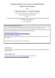
The following are a set of survival times 

(in days from entry to a trial) for patients 

with stage 3 diffuse hystiocytic lymphoma 

(from McKelvey, Gottlieb 1976, Cancer, 

38, 1484-1493). The graph on the right is 

the Kaplan—Meier product-limit (PL) 

graph of the data, commonly called the K- 

M plot, the vertical dashes represent the 

censored items, showing how the 

majority of them are at the far right of 

the graph as would be expected. In the 

table on the right I indicates the status 

(1=completed;0=censored) for each 

subject, alternatively often censored 

observations are indicated by a star, asterisk or + symbol. 

Notice that in our dataset 8 out of the 19 observations are 

not censored representing 50%. This is usually a good quick 

check to ensure you have used the censored / uncensored 

values the right way round, as the censored observations 

0 50 100 150 200 250 300 350 

Robin Beaumont robin@organplayers.co.uk D:\web_sites_mine\HIcourseweb new\stats\statistics2\part14_survival_analysis.docx page 3 of 22 

% surviving, S(t) 

0.0 0.2 0.4 0.6 0.8 1.0 

survival McKelvey et al., 1976 

Time (days )



do not affect the % surviving. Unfortunately 50% does not help matters much here as coding either way we 

will end up with a line at 50%, subsequent examples demonstrate this more successfully. Obviously the 

effective sample size decreases as we move from the left to the right of the K-M plot and this affects the 

accuracy of the estimates. Some authors provide a table along the bottom of the x axis or a separate one 

indicating the number of non-censored observations at several time points. 

Obviously, the lines on the K -M plot relate to a set of x,y values and investigating how these are calculated 

provides insight into what S(t) means, that is the values on the y axis. The table below shows how this is 

carried out. First lets consider some points of nomenclature. 

i = A time point, numbered on ordered survival times, from 0 to p, where p is equal to the number of 

cases/observations, there may be duplicate times (Machin, Campbell & Walters 2007 p.188) – they will rarely 

be equal. 

di = Number of cases failing at time ti 

ni = Number at risk just before time i [notice the downward pointing arrows in table below] 

ri= Number alive just before time i 

(ni-di)/ni = proportion surviving interval i =probability of surviving i [notice the horizontal arrows in table 

below] 

S(t) = probability of surviving from start (i=0) to ti = cumulative survival probability = Kaplan Meier Product 

limit estimator 

Failure time 

Ranked from shortest to largest, 

then uncensored,censored 

I 

di = No. failing at 

time ti 

ni = no. at risk 

ri= no. alive just 

before i 

(ni-di)/ni 

=proportion surviving 

interval i 

=probability of 

surviving i 

S(t) 

= probability of 

surviving from 

start (i=0) to ti 

= cumulative 

survival probability 

= Kaplan Meier 

Product limit 

estimator 

0 0 - 19 - 1 

6 1 

1 19 (19-1)/19= 

0.9474 

0.947 

19 2 1 19-1=18 

(18-1)/18= 

0.9444 

0.895 

32 3 

1 

18-1=17 

(17-1)17= 

0.9412 

0.842 

42 4 2 17-1=16 

(16-2)/16= 

0.8750 

0.737 

43* 5 0 16-2=14 1 

94 6 1 16-3=13 

(13-1)/13 

0.9231 

0.680 

126* 7 0 12 1 

169* 8 0 11 1 

207 9 1 11-1=10 

(10-1)/10 

0.9000 

0.612 

211* 10 0 9 1 

227* 11 0 8 1 

253 12 1 8-1=7 

(7-1)/7 

0.8571 

0.525 

There are three important aspects to note about the above: 

Current 

survival time i 

Up to time i 

• The proportion surviving in the penultimate column relates to the current survival time i –it is a 

conditional probability (Norman & Streiner 2008 p.278) 

• The S(t) function relates to all time intervals up to time i 

• The failure time ti is a value not an interval. This needs to measured accurately, requiring diligent 

follow-up and avoidance of relying upon recall from participants. 

Considering the last column a little more makes clear why the term 'product' is used when describing the S(t) 

function. It is calculated by multiplying (i.e. forming the product) all the previous proportions surviving for all 

the previous times so taking our 253 survival time (the largest non censored observation) 

S(t12) = 0.9474 x .9444 x .9412 x .8750 x .9231 x .9000 = .8571 (notice I have missed out the censored 

observations as x1 does nothing!) 




We can show this using the mathematical product (i.e. multiplication) operator ∏ so to indicate we want to 

multiply all the values for a particular expression from i=1 to i=12 we write: 

⎛n − d ⎞ 

= ∏ ⎜ ⎟ or more generally 

⎝ ⎠ 

( 12) 

12 

i= 1 

i 

ni 

i 

St 

j ⎛ni − d ⎞ i 

St ( j ) = ∏ ⎜ ⎟ 

i= 1 ⎝ ni 

⎠ 

Sometimes what appears to be a very frightening equation can underneath be something quite simple! All 

we are doing is multiplying the values for each period up to the time we require, its even simpler when we 

look at it graphically, considering the value for the 5 th and 9 th rows. 

. . . . . . 

. . . . . . 

. . . . . . 

. . . . . . 

. . . . . . 

. . . . . . 

. . . . . . 

. . . . . . 

. . . . . . 

. . . . . . 

. . . . . . 

. . . . . . 

. . . . . . 

. . . . . . 

. . . . . . 

. . . . . . 

. . . . . . 

. . . . . . 

. . . . . . 

. . . . . . 

. . . . . . 

. . . . . . 

. . . . . . 

. . . . . . 

decide if you think this adequately models your data. 

2.1 Producing a K-P plot in R 

If you have a knowledge of probability you may have realised that this is 

just the same as using the 'and' rule, for example the probability of 

throwing a 6 and then throwing another 6 with the usual dice is 1/6 x 

1/6 = 1/36 This illustrates another interesting fact about the model, the 

survival to time i is simply the product of all the individual conditional 

survival rates for each previous period. You as the researcher must 

As is usual with R there is an excellent free package to help you, called guess what, survival. The code below, 

largely taken from Malcolm Farrows excellent course illustrates how to produce the K-P plot given on the 

previous page for our dataset. 

library(survival) 

my.times

3. Several curves 

survival varies across different age bands etc. 



The nice thing about R, besides the 

free packages you can use with it ,is 

that they usually also contain very 

relevant datasets, for example the 

survival package contains a dataset 

called lung which is the survival 

time for 228 patients with lung 

cancer from the North Central 

Cancer Treatment group. The 

details are given opposite. 

Immediately you may think that it 

would be interesting to see if males 

and females differ in survival, or if 

But first it is always a good idea to explore the data before carrying out any sort of detailed analysis and the 

R code below demonstrates this. 

###################################### 

# the lung dataset in the survival package 

#first have a look at it 

# assuming you have the survival package installed 

# lung returns the data and headings, summary returns descriptive stats 

lung 

summary(lung) 

# names(lung) returns the list of column names: 

# [1] "inst" "time" "status" "age" "sex" "ph.ecog" 

# [7] "ph.karno" "pat.karno" "meal.cal" "wt.loss" 

names(lung) 

# if you dont know the names of the columns you can refer to each by subscript 

#lung[1] = lung$inst; lung[2] = lung$time etc 

#to list all the values in one column, say time: 

lung$time 

# be more use to see the number of censored to uncensored values 

# use the table function to produce a list of counts for each value 

temp1

0.0 0.2 0.4 0.6 0.8 1.0 



# now produce a K-P for the entire dataset, first creating 

the survival data object 

mylungsurv

Look at the survival curve for the combined data, then for the different tumour stagings. 

Make the curves different colours and line types. 

Add a legend and title to the K-P plot 



Inspect the data to evaluate if the following information is correct, at 253 days % surviving = 52.5 (stage 3); 

% surviving (stage 4) = about 25%; 

3.2 Comparing curves the Logrank and Beslow statistics 

The logrank statistic is formed by calculating the expected failures assuming that the groups are the same, 

which is then added up. The statistic then compares the observed against the expected values and carries 

out a chi square test on them. 

Function for Logrank test 

survdiff(mylungsurv~mylung$sex, rho = 0) 

Surv object 

0= Logrank statistic; 1= Gehan-Breslow statistic with 

Peto & Peto modification 

Grouping variable in dataset 

The problem with the Logrank statistic is that it does not take into account where the difference is in the 

survival curve, in other words it does not matter if there is a difference that changes over time, or may even 

reverse. In contrast the Gehan-Breslow statistic gives more weight to earlier differences in the dataset. In R 

you simply indicate which statistic you want with the "rho=" statement. 

The output below using the the lung data set, indicates that using the Logrank statistic we would have 

obtained data similar to that observed (i.e. producing our Logrank statistic) or that producing a more 

extreme Logrank statistic value just over once in every thousand times assuming the curves are just random 

samples from a single population. Similarly for the Gehan-Breslow statistic we can say that would have 

obtained data like that observed or more extreme just over three times in every ten thousand times 

assuming the curves are just random samples from a single population. If you take the statistic test approach 

you can then take this further by setting a critical value (usually 0.05) and decide to reject the assumption 

that they are just random samples from a single population (the null hypothesis) if the observed P value is 

less than the critical value, and instead 

accept that they must come from different 

populations (the alternative hypothesis). 

Using this approach, considering both 

associated probabilities we can reject the 

null hypothesis and come to the conclusion 

that the two curves are indeed not just 

displaying random sampling variability, but 

do come from different populations. 


Exercise 



Considering the histiocytic lymphoma tumour (stage 3 and 4) data discussed earlier. Use both the logrank 

and Breslow statistics to see if there is any statistically significant difference between the curves. 

Check these answers: time 253 days % surviving = 52.5 (stage 3); % surviving stage 4 = about 25%; logrank 

significant. 

We have now seen a way of comparing two or more survival curves, the next possibility is to consider the 

situation where there is some other variable that may also affect survival such as age etc. When this is the 

case we need to consider an approach that is like regression but with survival curves, while the mathematics 

behind this is complex we can consider a few salient features here. The most common type of survival 

regression is what is known as the Cox proportional hazards regression model. This chapter only provides the 

briefest of introductions to this topic, and excellent introductory chapters for the non statistician can be 

found in Norman & Streiner 2008 p.274 – 294 and Campbell & Swinscow 2009, or alternatively the article by 

Meier 1985 which although it is a little more statistical is very much concerned with medical matters. 

4. The Cox regression model 

The Cox regression model is just one of several approaches that attempts to evaluate survival curves taking 

into account other variables that may effect the survival (confounders/covariates/predictors etc). While 

Malcolm Farrows excellent course investigates several of them I will just provide a very short introduction to 

the Cox regression model here. 

The Cox model can be expressed a number of ways, and we will first look at the approach that defines it in 

terms of the cumulative survival function (S(t) i.e. the y axis on the K –M plot). Here we can say that the 

predicted survival at time t is equal to the baseline survival 

Survival = those who survive = 

taken to the power of an expression that contains the various 

predictors we might want to include. 

Survival at time t = Baseline survival 

St ( ) = [ S( t)] where p= e 

0 

p z 

To the power of the exponential expression 

containing the predictor values 

Survival is the optimistic side of the coin whereas the 

Hazard (i.e. death rate) is the flip side. 

Notice that we now have something similar to the 

logistic regression equation and you may remember 

that the beta's (β's) represented log odds ratios, 

however in the Cox model they represent the relative 

hazards (RH) which is also called the hazard ratios 

(HR). An example will make things clearer. 

While this format provides a conceptual framework back to 

the survival function the most common way of defining the 

model is by considering the Hazard function (represented by h 

or the lambda character λ) as the predicted value. The hazard 

can be thought of as the risk per unit time, and can vary 

between zero and infinity. Now the Cox model becomes: 

λ( t) = h ( t)exp( β x + β x +... + β x ) 

i 0 1 1 2 2 k k 

( β1x1+ β2x2+... + βkxk) 

i() 

= 0() 

h t h te 

Hazard = death rate = 

Hazard at time t = i Baseline hazard 

β's = Relative risks =hazard ratios 

The data on the next page (Collett 1994, p291) 

represents information from 26 ovarian cancer chemotherapy patients treated with cyclophosphamide (the 

monotherapy group) or a mixture of cyclophosphamide and adriamycin (the combined therapy group), along 

with their age and outcome. The K-M plot on the next page suggests that the monotherapy group do worse 

at any stage of followup. Also we could calculate the Logrank or Gehan-Breslow statistics and inspect the 

associated p values to see if this is possibly the case. 


Exercise 



Considering the Ovarian cancer data below produce a K –M plot along with Logrank and Gehan-Breslow 

statistics. What conclusions do you come to? Which of the p values is equal to .303 and .194? 

Ovarian cancer data (Collett 1994 p.290) 

[survival_collett_p290.sav] 

Subject no time 

Cens 

[censored = 0] 

Treat [1=single; 

2=combination] 

Age [years] 

1 156 1 1 66 

2 1040 0 1 38 

3 59 1 1 72 

4 421 0 2 53 

5 329 1 1 43 

6 769 0 2 59 

7 365 1 2 64 

8 770 0 2 57 

9 1227 0 2 59 

10 268 1 1 74 

11 475 1 2 59 

12 1129 0 2 53 

13 464 1 2 56 

14 1206 0 2 44 

15 638 1 1 56 

16 563 1 2 55 

17 1106 0 1 44 

18 431 1 1 50 

19 855 0 1 43 

20 803 0 1 39 

21 115 1 1 74 

22 744 0 2 50 

23 477 0 1 64 

24 448 0 1 56 

25 353 1 2 63 

26 377 0 2 58 

Exercise 

It is always a good idea to 

use the table command 

to check quickly the 

degree of censoring in 

each group, as shown 

opposite. We would also 

check the mean/median 

age for each group. 

mydata



After having created the Surv object for 

displaying the K-M plot we simply use it 

as the outcome variable in the formula 

for the Cox regression model: 

my_coxph



You can also compare the models for each 

of the predictors separately; the 

screenshot opposite gives the details. 

5. Using Spss 

Obtaining a K-M plot and Cox regression 

analysis in SPSS is remarkably simple. Chan 

Yiong Huak, Head of the Biostatistics Unit, 

Yong Loo Lin School of Medicine, National 

University of Singapore, (Chan Y H 2004a) 

provides an excellent tutorial for Cox 

regression. 

Exercise 

Download the Chan, 2004 article at: 

http://www.sma.org.sg/smj/4506/4506bs1.pdf 

The data you need to carry out the K-P plot is provided on the right hand column of the first page and 

censoring details on the following page. However the enhanced lung cancer dataset is not available for the 

subsequent pages, But I have provided a set of data from the 1973 Prentice lung cancer study 

[lung_cancer_prentice1973.sav]. In contrast the Breast cancer dataset (p.254) is available for the second 

part of the article as it is part of SPSS (called breast_cancer_survival.sav) 

The alternative much used Lung cancer dataset (taken from Prentice (1773) and reproduced in Kalbßeisch & 

Prentice 1980 can also be found at the Central University of Michigan University SPSS On-line Training 

Workshop under the survival analysis category at http://www.cst.cmich.edu/users/lee1c/spss/toc.htm along 

with a excellent video demonstrating how to analyse the dataset at 

http://www.cst.cmich.edu/users/lee1c/spss/V16_materials/Video_Clips_v16/40CoxRegression/40CoxRegres 

sion.swf 

6. Interpreting the beta's (β) 

The Hazard Ratio (HR) is exp(β) and is the relative hazard corresponding to a unit change in the associated 

predictor. In this instance you can think of a hazard as a death rate, so greater the number the worse the 

outcome. 

 

Hazard ratio (risk ratio) – how to interpret it 

Taking each of the predictors separately, 

for the ovarian cancer dataset: 

age: using the last model in the r console 

screenshot above, 1.158 is the HR of 

death in a subject (i.e. woman) of age a + 1 years relative to that of a woman of age a. As in the case with 

logistic regression we can also consider multiple years such as (1.158) 5 = 2.082298 so if you are five years 

older your odds or dying are twice that of that someone 5 years your junior, similarly if you are 10 years 

older it goes up to (1.158) 10 < 1 

> 1 

= 4.335963, that is your odds of dying are over 4 times that of someone 10 years 

younger. 

 


i 0 treat _iage _ii 0 



group: taking the last model again, 0.451 is the HR of death in a subject (i.e. woman) in group 2 (combined 

therapy) relative to that of a subject on monotherapy (group=1), Collett 1994 p297. This is because for 

nominal predictor variables (covariates) one category is the 'reference group' which means that it has a 

coefficient of 1, in other words the single therapy has a hazard ratio of 1. 

In reality we would probably remove the 'group' predictor from the equation as it's associated p value is 

not significant but for the purpose of the following exercises we will assume that it is significant. 

7. Hazard ratios, odds and probabilities 

There is a danger of misinterpreting the Hazard Ratio (HR) and two common misinterpretations are 

comparing values and relating the values to time to the event. For example thinking that a HR of 2 versus 1 

means that the subject has twice the chance (i.e. probability) of succumbing to the event or that the time to 

get to the event is halved, none of these interpretations are correct. See the clear excellent article by 

Spruance & Reid et al 2004, p. 2790 for full details. 

HR probability 

0.5 0.33 

0.6 0.38 

0.7 0.41 

0.8 0.44 

0.9 0.47 

1 0.50 

1.1 0.52 

1.2 0.55 

1.3 0.57 

1.4 0.58 

1.5 0.60 

2 0.67 

3 0.75 

4 0.80 

5 0.83 

6 0.86 

7 0.88 

8 0.89 

9 0.90 

10 0.91 

The best way to think about Hazard Ratios is to think about odds, and once again using the 

material in the simple logistic regression chapter we can convert the odds, in this instance 

HR's, to probabilities. 

pi odds 

p 

In this context: 

i HR 

odds = ⇒ pi 

= 

HR = ⇒ pi 

= 

1− p 1+ 

odds 

1− p 1+ 

HR 

Looking at the table opposite we can see that a hazard ratio of 2 therefore corresponds to a 

67% greater chance of reaching the event compared to the other group, and a hazard ratio of 

3 corresponds to a 75% chance of reaching the event first. Clearly this can be both a good and 

bad thing depending upon what the event is! For our ovarian cancer dataset we have a HR of 

2.08 for an increase in age of 5 years and 4.33 for a 10 year increase in age, using the table 

opposite as a rough and ready estimator we see that this corresponds to a increased 

probability of death of 67% for five years and 80% for ten years. 

8. Finding individual HR scores 

As we did in both simple regression and logistic regression, now we know the values of the β's we can 

substitute the values for a specific subject and get a predicted hazard ratio value back, however there 

appears one small problem, we do no know the value of the baseline hazard and this is not calculated via the 

Cox model so all we have is the relative hazard to some theoretical baseline risk group, luckily this is not 

usually a problem. Taking our Ovarian cancer data, lets consider two scenarios, the hazard for a 30 yr old 

receiving mono-therapy (=1) and a 60 year old receiving combination therapy (=0) 

Taking the 30 yr old receiving mono-therapy (=1): 

0.451xtreat _i1.158xage _i 

λ ( t) = h ( t)exp(0.451 x +1.158 x ) ⇒ h( t) = h ( t)( e )( e ) 

hi() t = h ()( t e 

= h ( t)(3.788) 

)( e ) ⇒h ()( t e )( e ) ⇒h () t e ⇒h 

() t e 

0 

i 

(0.451)(1) (1.158)(30) (0.451) 34.74 .451+ 43.74 44.191 

0 0 0 0 

So the hazard for our 30 year old on mono-therapy is just under 4 times the baseline risk. You may be 

wondering why the '+'s become multiplication this is because one of the rules of exponents which states that 

x (a+b+c) =x a x b x c . Think about it this way 2 2 =(2)(2) and also 2 3 =(2)(2)(2) = 2 (1+1+1) Also incientially x 0 = 1, so any 

covariate that has a zero value for beta means that the value in effect represents a multiplier of one so it 

have no effect on the baseline hazard as would be expected. Our 3.788, using the HR/probability table is 

equivalent to an increase in risk of 80%. 


i

Taking the 60 year old receiving combination therapy (=0): 



(0.451)(0) (1.158)(60) (0.451) 34.74 0+ 69.48 69.48 

hi() t = h0()( t e )( e ) ⇒h0()( t e )( e ) ⇒h0() t e ⇒h0() 

t e 

= h0( t)(4.241) 

So the hazard for our 60 year old on combination therapy is just over 4 times the baseline risk and once again 

equals a increase in risk of around 80% 

9. Assumptions, dangers and assessment of Cox regression 

This chapter was intended as a very brief introduction to the model. We have not discussed in detail the 

ways the K-P plot can be abused, Pocock Clayton & Altman, 2002 discuss in detail the common problems 

found with K-P plots and how to avoid them. 

For Cox regression to produce valid results, there are several assumptions that the model makes, these are 

described well in both Campbell 2006 and Norman & Streiner 2009. Peat, Burton and Elliott, 2009 provide 

two check lists, one concerning the assumptions for carrying out a valid Cox regression (provided below) and 

another one listing issues to consider when reviewing an article concerning survival analysis. 

Assumptions for standard survival analysis (from Peat, Barton & Elliott 

2008 p.131, adapted) 

• Observations are independent, each person is only included once 

• Survival prospects remain constant over the study period 

(although this can be modelled used advanced techniques) 

• Censored observations have the same survival prospects as the 

non-censored participants 

• Degree of censoring and sample size needs to be considered. 


10. Multiple choice Questions 

1. Burton and Walls 1987 investigated the survival of patients 

on one of three types of renal replacement therapy, peritoneal 

dialysis, heamodialysis and transplantation details given 

opposite. What is the usual name for the exponential 

coefficient column? (one correct choice) 

a. Hazard Rate (HR) 

b. 

c. Hazard Ratio (HR) 

d. Hazard probability 

e. Hazard proportion 

f. Hazard logarithm 

2. Considering the results from Burton and Walls 1987 given 

opposite. Which is the most appropriate way of interpreting 

the values in the exponential coefficient column (one correct 

choice) 

a. Odds 

b. Probability 

c. Time to event 

d. Proportion failing 

e. Odds ratio 



3. Considering the results from Burton and Walls 1987 given above. Which variable represents the greatest hazard (one correct 

choice) 

a. Age (in decades) 

b. Amyloidosis 

c. Convulsions 

d. Ischaemic heart disease 

e. Acute or acute on chronic presentation 

4. Considering the results from Burton and Walls 1987 given above. Which variable represents the greatest benefit (one correct 

choice) 

a. Male sex 

b. Parenthood 

c. Pyenonephritis 

d. Residence in Leicestershire 

e. Absence of Ischaemic heart disease 

5. Considering the results from Burton and Walls 1987 given above. If anyone were considering dropping a variable from the model 

which one would it most likely be? (one correct choice) 

a. Male sex 

b. Parenthood 

c. Pyenonephritis 

d. Residence in Leicestershire 

e. Absence of Ischaemic heart disease 

6. Considering the results from Burton and Walls 1987 given above. What is the Exponential coefficient value likely going to be for the 

female sex? (one correct choice) 

a. 0 

b. .5 

c. 1 

d. 1- 0.48 

e. 1+ 0.48 

Burton P R, Walls J 1987 Selection-adjusted comparison of life-expectancy of patients 

on continuous ambulatory peritoneal dialysis, haemodialysis, and renal 

transplantation 

Variables that significantly influenced probability of survival 

Variable 

Exponential coefficient 

(risk multiplying factor) 

Statistical 

significance 

Adverse 

Age (each additional decade) 1.68 p

7. Considering the results from Rait et al 2010 given opposite. What is the 

more usual term for the x axis? (one correct choice) 

a. Survival function S(t) 

b. Logit 

c. Inverse hazard 

d. Actuarial survival 

e. Proportion censored 

8. Considering the results from Rait et al 2010 given opposite. The cohort 

detail below the x axis are? (one correct choice) 

a. Irrelevant and should not be shown 

b. Confuse the issues 

c. More important than the graph 

d. Provide useful additional information 

e. Can be calculated from the graph 



9. When gathering the failure times to calculate the Kaplan Meier plot which of the following statements is correct? (one correct 

choice) 

a. Its accurate measurement is of minimal importance 

b. Can be grouped into equal intervals 

c. Can be calculated from other measures 

d. Its accurate measurement is of major importance 

e. It is best to collect then at the end of the study period only 

10. Censored observations do not include . . .? (one correct choice) 

a. Those who experience the event during the followup period of the study 

b. Those that are lost to followup 

c. Those that fail to provide event data 

d. Those subjects whose survival time is less than the followup period of the study 

e. Those who experience the event after the followup period of the study 

11. Censored observations are . . .? (one correct choice) 

a. More important than non-censored ones in survival analysis 

b. Are assumed to be normally distributed over time 

c. Are assumed to have the same survival chances as uncensored observations 

d. Are essential to allow calculation of the Kaplan Meier plot 

e. Are allocated to the baseline survival curve 

12. A Cox regression analysis . . .(one correct choice) 

a. Is used to analyse survival data when individuals in the study are followed for varying lengths of time. 

b. Can only be used when there are censored data 

c. Always assumes that the relative hazard for a particular variable is constant at all times 

d. Uses the logrank statistic to compare two survival curves 

e. Relies on the assumption that the explanatory variables (covariates) in the model are Normally distributed. 

(taken from p. 210) 


11. Exercises 



Questions 1 to 3 are about dentistry issues, question 4 is for veterinary students and question 5 for 

psychologists, but obviously interested students can consider other areas. 

1 The following data represent implant survival times (in months) for 15 smokers with low bone density (less 

than 65%). Construct the Kaplan- Meier product limit estimator. What is the standard error for the Kaplan- 

Meier 

55.4+ 89.0 112.5+ 84.7 98.4 23.5+ 62.0 98.4+ 102.5 68.0 46.8+ 68.0 23.5+ 112.0 92.1+ 3 

(From Kime & Dailey 2008 p.298) 

2 Smoking is believed to be a significant risk factor for the lifetime of implants. As part of a class project, a 

team of three dental students examined 21 patient charts and obtained the following data. 

Perform a log rank test at the significance level of α = 0.05 to confirm if the claim is justified. 

Smokers: 45.3+ 98.5 74.0+ 68.2 32.6 103.0+ 87.2 110.4 

Non-smokers: 72.0+ 48.4+ 113.5 95.0 82.9+ 78.6+ 125.0 110.0 95.0+ 72.0+ 132.8 52.8+ 106.5 


3 Acidulated fluoride preparations may corrode the surface of titanium implants. Thus, patients with this 

type of implant are generally recommended to avoid fluoride use. The 10-year followup investigation of the 

patients with titanium implants placed in the maxillary anterior region obtained the survival data shown 

below. 

14.5+ 21.4+ 33.0 40.8 58.5 58.5+ 69.8 70.2 77.5+ 85.0 89.5 94.0 94.0+ 94.0+ 97.0 99.5 103.8 105.5+ 105.5+ 

108.4 110.0 115.8+ 118.0 


4. Lord, Griffin & Slater et al 2010 evaluated the effectiveness of collars and microchips for visual and 

permanent identification of pet cats using survival analysis techniques including Cox regression to compare 

various covariates. Download the article and consider the following: 

• What unique problems are associated with the event in this research compared to the human 

research discussed earlier? 

• Several groups have a HR of 1 what technically are these groups called? 

• How do you think the research design could be extended/improved 




5. The data below is a subset of data recorded in a study of the relationship among pubertal development, 

sexual milestones, and childhood sexual abuse in women with eating disorders (Schmidt, Evans, Tiller, & 

Treasure, 1995, quoted in Landau 2002). The data considered here represent times to first sexual intercourse 

for two groups of women. The first group consisted of a 

consecutive series of female outpatients who presented to 

an eating disorder unit and fulfilled the criteria for 

restricting anorexia nervosa (RAN). The second group was 

a reference group of female polytechnic students who 

were approached in the college canteen during break time 

("controls"). Some women had not experienced sex by the 

time they filled out the study questionnaire; their event 

times were therefore censored at their age at the time of 

the study. Such observations are marked by a "+" Analyse 

the data using both Kaplan Meier plot and cox regression. 

What conclusions do you come to. If possible also 

download the Landau article to compare your analysis with 

Lanau's. 

Participant 

Group (code 

RAN=1;control=0) 

Time (age of first 

sexual 

intercourse) 


Age 

(years) 

status 

1 RAN 30+ 30 Censored 


3 RAN 12 18 Event 






































41 Control 15 20 Event 







4B Control 16 20 Event 




















68 Control 18+ 18 Censored 
















84 Control 18 21 Event

12. Summary 



This chapter introduced survival analysis which is unique in allowing the analysis of censored data. We firstly 

considered the Kaplan Meier Plot and than the more complex Cox regression model. Similarities to the 

approach described in the simple logistic regression model were highlighted. 

Whereas in previous chapters a full explanation was given of carrying out the analysis in both R and SPSS, in 

this chapter the SPSS analysis was left as a directed exercise. 

Survival analysis is not just a major aspect of medical statistics, being used in 32% of the papers in the New 

England journal of Medicine (Altman, 1991) but also being used in the veterinary (Lord, Griffin & Slater et al 

2010; Lee & Wang 2003) and psychology (Landau 2002) fields. 

The Cox model has been extended over the years to accommodate additional complexities which we have 

not considered here and clearly if you are considering a study that involves survival analysis techniques you 

should obtain statistical advice at the start of the study. 

13. References 

Altman D G, PK Andersen P K. 1999 Calculating the number needed to treat for trials where the outcome is 

time to an event, BMJ 319 1492–1495. 

Altman, D. G. 1991 Statistics in medical journals: Developments in the 1980’s. Stat Med; 10, 1897–1913. 

Burton P R, Walls J 1987 Selection-adjusted comparison of life-expectancy of patients on continuous 

ambulatory peritoneal dialysis, haemodialysis, and renal transplantation. The Lancet. 329 (8542) [16 May] 

1115-1118 1987 

Chan Y H 2004 Biostatistics 203: Survival analysis [using spss]. Basic statistics for Doctors. Singapore Med J 

45(6) 249. Open access: http://www.sma.org.sg/smj/4506/4506bs1.pdf 

Collett D 1994 Modelling survival data in medical research (Chapman & Hall/CRC) [second edition 2003 omits 

chapter on software packages] 

Crawley M J 2005 Statistics: An introduction using R. Wiley 

Kim J S, Dailey R J, 2008 Biostatistics for oral Healthcare. Blackwell 

Kalbßeisch J, Prentice R 1980 The Statistical Analysis of Failure ¹ime Data, Wiley, New York, 1980. Veterans 

Administration lung cancer trial data (Prentice 1973), listed on pp. 223 - 224 

Landau S 2002 Using Survival Analysis in Psychology. Understanding statistics, 1(4), 233-270 

Lee E T, Wang J W 2003 (3 rd ed) Statistical methods for survival data analysis. Wiley 

Lord l K, Griffin B, Slater M R, J K Levy 2010 Evaluation of collars and microchips for visual and permanent 

identification of pet cats. JAVMA, 237 (4) [August 15] 387-394 

McKelvey M. Gottlieb JA et al 1976 Hydroxydaunomycin (Adriamycin) combination chemotherapy in 

malignant lymphoma. Cancer 38 1484 – 1493 

Meier P 1985 Anatomy and Interpretation of the Cox regression model. Asaio journal 8 3-12 

Norman G R, Streiner D L. 2008 (3 rd ed) Biostatistics: The bare Essentials. 

Peat J, Burton B, Elliott E 2009 statistics workbook for evidence based healthcare. 

Petrie A. P Watson 2006 (2 nd ed) Statistics for Veterinary and animal science. Blackwell. 




Pocock J S, Clayton T C, Altman D G. 2002 Survival plots of time-to-event outcomes in clinical trials: good 

practice and pitfalls. Lancet 359 [May 11] 1686–89 

Prentice R L 1973 Exponential survival with censoring and explanatory variables . Biometrika 60 : 279 – 288 

Rait G, Walters K, Bottomley C, Petersen I, Iliffe S, Nazareth I. 2010 Survival of people with clinical diagnosis 

of dementia in primary care: cohort study. BMJ 341 c3584. Open access. 

Spruance S L, Reid J E, Grace M, Samore M. 2004 Hazard Ratio in clinical trials. Antimicrobial agents and 

chemotherapy. 48 (8) [Aug. 2004] p.2787–2792. Open access at: http://aac.asm.org/cgi/reprint/48/8/2787 

Tibshirani R 1997 The Lasso Method For Variable Selection In The Cox Model. Statistics In Medicine, Vol. 16, 

385-395 


14. Appendix r code 



##################### basic survival analysis 

# first draw create the Surv object so that we can create the Kaplan Meier plot (K-M plot) 

# but first need to load the survival library 

library(survival) 

my.times

summary(my_coxph) 

my_coxphnull

An Introduction to statistics Survival Analysis 1

Create successful ePaper yourself

Delete template?

Save as template?