6 Extravascular routes of drug administration
6 Extravascular routes of drug administration
6 Extravascular routes of drug administration

Create successful ePaper yourself
Turn your PDF publications into a flip-book with our unique Google optimized e-Paper software.
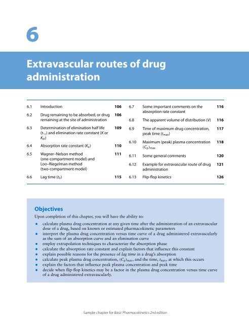
6<br />
<strong>Extravascular</strong> <strong>routes</strong> <strong>of</strong> <strong>drug</strong><br />
<strong>administration</strong><br />
6.1 Introduction 106<br />
6.2 Drug remaining to be absorbed, or <strong>drug</strong><br />
remaining at the site <strong>of</strong> <strong>administration</strong><br />
6.3 Determination <strong>of</strong> elimination half life<br />
(t1/2) and elimination rate constant (K or<br />
Kel)<br />
106<br />
109<br />
6.4 Absorption rate constant (Ka) 110<br />
6.5 Wagner–Nelson method<br />
(one-compartment model) and<br />
Loo–Riegelman method<br />
(two-compartment model)<br />
111<br />
6.6 Lag time (t0) 115<br />
Objectives<br />
Upon completion <strong>of</strong> this chapter, you will have the ability to:<br />
6.7 Some important comments on the<br />
absorption rate constant<br />
116<br />
6.8 The apparent volume <strong>of</strong> distribution (V) 116<br />
6.9 Time <strong>of</strong> maximum <strong>drug</strong> concentration,<br />
peak time (tmax)<br />
6.10 Maximum (peak) plasma concentration<br />
(Cp)max<br />
117<br />
118<br />
6.11 Some general comments 120<br />
6.12 Example for extravascular route <strong>of</strong> <strong>drug</strong><br />
<strong>administration</strong><br />
121<br />
6.13 Flip-flop kinetics 126<br />
• calculate plasma <strong>drug</strong> concentration at any given time after the <strong>administration</strong> <strong>of</strong> an extravascular<br />
dose <strong>of</strong> a <strong>drug</strong>, based on known or estimated pharmacokinetic parameters<br />
• interpret the plasma <strong>drug</strong> concentration versus time curve <strong>of</strong> a <strong>drug</strong> administered extravascularly<br />
as the sum <strong>of</strong> an absorption curve and an elimination curve<br />
• employ extrapolation techniques to characterize the absorption phase<br />
• calculate the absorption rate constant and explain factors that influence this constant<br />
• explain possible reasons for the presence <strong>of</strong> lag time in a <strong>drug</strong>’s absorption<br />
• calculate peak plasma <strong>drug</strong> concentration, (Cp)max, and the time, tmax, at which this occurs<br />
• explain the factors that influence peak plasma concentration and peak time<br />
• decide when flip-flop kinetics may be a factor in the plasma <strong>drug</strong> concentration versus time curve<br />
<strong>of</strong> a <strong>drug</strong> administered extravascularly.<br />
Sample chapter for Basic Pharmacokinetics 2nd edition
106 Basic Pharmacokinetics<br />
6.1 Introduction<br />
Drugs, through dosage forms, are most frequently<br />
administered extravascularly and the majority <strong>of</strong> them<br />
are intended to act systemically; for this reason,<br />
absorption is a prerequisite for pharmacological<br />
effects. Delays or <strong>drug</strong> loss during absorption may<br />
contribute to variability in <strong>drug</strong> response and, occasionally,<br />
may result in a failure <strong>of</strong> <strong>drug</strong> therapy.<br />
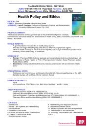
The gastrointestinal membrane separates the absorption<br />
site from the blood. Therefore, passage <strong>of</strong><br />
<strong>drug</strong> across the membrane is a prerequisite for absorption.<br />
For this reason, <strong>drug</strong> must be in a solution<br />
form and dissolution becomes very critical for the<br />
absorption <strong>of</strong> a <strong>drug</strong>. The passage <strong>of</strong> <strong>drug</strong> molecules<br />
from the gastrointestinal tract to the general circulation<br />
and factors affecting this are shown in Figs 6.1<br />
and 6.2. Any factor influencing dissolution <strong>of</strong> the<br />
<strong>drug</strong> is likely to affect the absorption <strong>of</strong> a <strong>drug</strong>. These<br />
factors will be discussed, in detail, later in the text.<br />
Drug, once in solution, must pass through membranes<br />
before reaching the general circulation. Hence,<br />
the physicochemical properties <strong>of</strong> the <strong>drug</strong> molecule<br />
(pKa <strong>of</strong> the <strong>drug</strong>, partition coefficient <strong>of</strong> the <strong>drug</strong>, <strong>drug</strong><br />
solubility, etc.), pH at the site <strong>of</strong> <strong>drug</strong> <strong>administration</strong>,<br />
nature <strong>of</strong> the membrane, and physiological factors<br />
will also influence the absorption <strong>of</strong> a <strong>drug</strong>.<br />
The present discussion will deal with general principles<br />
that determine the rate and extent <strong>of</strong> <strong>drug</strong><br />
absorption and the methods used to assess these<br />
and other pharmacokinetic parameters, from plasma<br />
concentration versus time data following oral <strong>administration</strong><br />
<strong>of</strong> <strong>drug</strong>s. Emphasis is placed upon absorption<br />
<strong>of</strong> <strong>drug</strong>s following oral <strong>administration</strong> because it<br />
illustrates all sources <strong>of</strong> variability encountered<br />
during <strong>drug</strong> absorption.<br />
Note that a similar approach may be applied to<br />
determine pharmacokinetic parameters <strong>of</strong> <strong>drug</strong>s when<br />
any other extravascular route is used.<br />
The following assumptions are made.<br />
• Drug exhibits the characteristics <strong>of</strong> onecompartment<br />
model.<br />
• Absorption and elimination <strong>of</strong> a <strong>drug</strong> follow<br />
the first-order process and passive diffusion is<br />
operative all the time.<br />
• Drug is eliminated in unchanged form (i.e., no<br />
metabolism occurs).<br />
• Drug is monitored in the blood.<br />
Useful pharmacokinetic parameters<br />
Figure 6.3 outlines the absorption <strong>of</strong> a <strong>drug</strong> that fits a<br />
one-compartment model with first-order elimination.<br />
The following information is useful:<br />
1 equation for determining the plasma concentration<br />
at any time t<br />
2 determination <strong>of</strong> the elimination half life (t1/2)<br />
and rate constant (K or Kel)<br />
3 determination <strong>of</strong> the absorption half life (t1/2)abs<br />
and absorption rate constant (Ka)<br />
4 lag time (t0), if any<br />
5 determination <strong>of</strong> the apparent volume <strong>of</strong> distribution<br />
(V or Vd) and fraction <strong>of</strong> <strong>drug</strong> absorbed<br />
(F)<br />
6 determination <strong>of</strong> the peak time (tmax)<br />
7 determination <strong>of</strong> the peak plasma or serum concentration<br />
(Cp)max.<br />
6.2 Drug remaining to be<br />
absorbed, or <strong>drug</strong> remaining at<br />
the site <strong>of</strong> <strong>administration</strong><br />
Equation (6.1) describes the changes in mass <strong>of</strong> absorbable<br />
<strong>drug</strong> over time at the site <strong>of</strong> <strong>administration</strong>.<br />
−dXa<br />
dt = Ka(Xa)t (6.1)<br />
where −dX/dt is the decrease in the amount <strong>of</strong> absorbable<br />
<strong>drug</strong> present at the site <strong>of</strong> <strong>administration</strong> per<br />
unit time (e.g., mg h −1 ); Ka is the first-order absorption<br />
rate constant (h −1 ; min −1 ); and (Xa)t is the mass<br />
or amount <strong>of</strong> absorbable <strong>drug</strong> at the site <strong>of</strong> <strong>administration</strong><br />
(e.g., the gastrointestinal tract) at time t.<br />
Upon integration <strong>of</strong> Eq. (6.1), we obtain the following:<br />
(Xa)t = (Xa)t=0e −Kat = FX0e −Kat<br />
Sample chapter for Basic Pharmacokinetics 2nd edition<br />
(6.2)<br />
where (Xa)t=0 is the mass or amount <strong>of</strong> absorbable<br />
<strong>drug</strong> at the site <strong>of</strong> <strong>administration</strong> at time t = 0 (for<br />
extravascular <strong>administration</strong> <strong>of</strong> <strong>drug</strong>, (Xa)t=0 equals<br />
FX0); F is the fraction or percentage <strong>of</strong> the administered<br />
dose that is available to reach the general<br />
circulation; and X0 is the administered dose <strong>of</strong><br />
<strong>drug</strong>.<br />
If F = 1.0, that is, if the <strong>drug</strong> is completely<br />
(100%) absorbed, then<br />
(Xa)t = X0e −Kat . (6.3)
Figure 6.1 Barriers to gastrointestinal absorption.<br />
Both Eqs (6.2) and (6.3) and Fig. 6.4 clearly indicate<br />
that the mass, or amount, <strong>of</strong> <strong>drug</strong> that remains<br />
at the absorption site or site <strong>of</strong> <strong>administration</strong> (or<br />
remains to be absorbed) declines monoexponentially<br />
with time.<br />
However, since we cannot measure the amount<br />
<strong>of</strong> <strong>drug</strong> remaining to be absorbed (Xa) directly, because<br />
<strong>of</strong> practical difficulty, Eqs (6.2) and (6.3), for<br />
the time being, become virtually useless for the purpose<br />
<strong>of</strong> determining the absorption rate constant;<br />
and, therefore, we go to other alternatives such as<br />
monitoring <strong>drug</strong> in the blood and/or urine to determine<br />
the absorption rate constant and the absorption<br />
characteristics.<br />
Monitoring <strong>drug</strong> in the blood<br />
(plasma/serum) or site <strong>of</strong> measurement<br />
The differential equation that follows relates changes<br />
in <strong>drug</strong> concentration in the blood with time to the<br />
<strong>Extravascular</strong> <strong>routes</strong> <strong>of</strong> <strong>drug</strong> <strong>administration</strong> 107<br />
absorption and the elimination rates:<br />
Sample chapter for Basic Pharmacokinetics 2nd edition<br />
dX<br />
dt = KaXa − KX (6.4)<br />
where dX/dt is the rate (mg h −1 ) <strong>of</strong> change <strong>of</strong> amount<br />
<strong>of</strong> <strong>drug</strong> in the blood; X is the mass or amount <strong>of</strong><br />
<strong>drug</strong> in the blood or body at time t; Xa is the mass<br />
or amount <strong>of</strong> absorbable <strong>drug</strong> at the absorption site<br />
at time t; Ka and K are the first-order absorption and<br />
elimination rate constants, respectively (e.g., h −1 );<br />
KaXa is the first-order rate <strong>of</strong> absorption (mg h −1 ,<br />
µg h −1 , etc.); and KX is the first-order rate <strong>of</strong> elimination<br />
(e.g., mg h −1 ).<br />
Equation (6.4) clearly indicates that rate <strong>of</strong><br />
change in <strong>drug</strong> in the blood reflects the difference<br />
between the absorption and the elimination rates (i.e.,<br />
KaXa and KX, respectively). Following the <strong>administration</strong><br />
<strong>of</strong> a dose <strong>of</strong> <strong>drug</strong>, the difference between the<br />
absorption and elimination rates (i.e., KaXa − KX)<br />
becomes smaller as time increases; at peak time, the<br />
difference becomes zero.
108 Basic Pharmacokinetics<br />
Figure 6.2 Passage <strong>of</strong> <strong>drug</strong> in the gastrointestinal tract until transport across the membrane.<br />
X a<br />
(Absorbable<br />
<strong>drug</strong> at absorption<br />
site)<br />
X a<br />
K a (h –1 )<br />
Absorption<br />
K a<br />
SCHEME:<br />
X<br />
(<strong>drug</strong> in<br />
body or<br />
blood)<br />
SETUP:<br />
X<br />
K<br />
K (h –1 )<br />
Elimination<br />
Figure 6.3 Absorption <strong>of</strong> a one-compartment <strong>drug</strong> with first-order elimination, where Xa is the mass or amount <strong>of</strong> absorbable<br />
<strong>drug</strong> remaining in the gut, or at the site <strong>of</strong> <strong>administration</strong>, at time t (i.e., <strong>drug</strong> available for absorption at time t); X is the mass or<br />
amount <strong>of</strong> <strong>drug</strong> in the blood at time t; Xu is the mass or amount <strong>of</strong> <strong>drug</strong> excreted unchanged in the urine at time t; Ka is the<br />
first-order absorption rate constant (h −1 or min −1 ); and K (or Kel) is the first-order elimination rate constant (h −1 or min −1 ).<br />
Sample chapter for Basic Pharmacokinetics 2nd edition<br />
X u<br />
X u
(a) (b)<br />
X a (mg)<br />
t = 0<br />
Time (h)<br />
X a (mg)<br />
t = 0<br />
<strong>Extravascular</strong> <strong>routes</strong> <strong>of</strong> <strong>drug</strong> <strong>administration</strong> 109<br />
Intercept = (X a ) 0 or FX 0<br />
Time (h)<br />
Slope = –K a<br />
2.303<br />
Figure 6.4 Amount <strong>of</strong> <strong>drug</strong> remaining at the site <strong>of</strong> <strong>administration</strong> against time in a rectilinear plot (a) and a semilogarithmic<br />
plot (b). Xa, amount <strong>of</strong> absorbable <strong>drug</strong> at the site <strong>of</strong> <strong>administration</strong>; (Xa)0, amount <strong>of</strong> absorbable <strong>drug</strong> at the site <strong>of</strong><br />
<strong>administration</strong> at time t = 0; F, fraction <strong>of</strong> administered dose that is available to reach the general circulation.<br />
Note that, most <strong>of</strong> the time, the absorption<br />
rate constant is greater than the elimination rate constant.<br />
(The exceptional situation when K > Ka, termed<br />
“flip-flop kinetics,” will be addressed in Section 6.13.)<br />
Furthermore, immediately following the <strong>administration</strong><br />
<strong>of</strong> a dose <strong>of</strong> <strong>drug</strong>, the amount <strong>of</strong> (absorbable)<br />
<strong>drug</strong> present at the site <strong>of</strong> <strong>administration</strong> will be<br />
greater than the amount <strong>of</strong> <strong>drug</strong> in the blood. Consequently,<br />
the rate <strong>of</strong> absorption will be greater than the<br />
rate <strong>of</strong> elimination up to a certain time (prior to peak<br />
time); then, exactly at peak time, the rate <strong>of</strong> absorption<br />
will become equal to the rate <strong>of</strong> elimination. Finally,<br />
the rate <strong>of</strong> absorption will become smaller than<br />
the rate <strong>of</strong> elimination (post peak time). This is simply<br />
the result <strong>of</strong> a continuous change in the amount <strong>of</strong> absorbable<br />
<strong>drug</strong> remaining at the site <strong>of</strong> <strong>administration</strong><br />
and the amount <strong>of</strong> <strong>drug</strong> in the blood. Note also that<br />
rate <strong>of</strong> absorption and the rate <strong>of</strong> elimination change<br />
with time (consistent with the salient feature <strong>of</strong> the<br />
first-order process), whereas the absorption and the<br />
elimination rate constants do not change.<br />
Integration <strong>of</strong> Eq. (6.4) gives<br />
(X)t = Ka(Xa)t=0<br />
Ka − K (e−Kt − e −Kat )<br />
= KaFX0<br />
Ka − K (e−Kt − e −Kat ) (6.5)<br />
where (X)t is the mass (amount) <strong>of</strong> <strong>drug</strong> in the body<br />
at time t; X0 is the mass <strong>of</strong> <strong>drug</strong> at the site <strong>of</strong> <strong>administration</strong><br />
at t = 0 (the administered dose); F is the<br />
fraction <strong>of</strong> <strong>drug</strong> absorbed; (Xa)0 = FX0 and is the<br />
Sample chapter for Basic Pharmacokinetics 2nd edition<br />
mass <strong>of</strong> administered dose that is available to reach<br />
the general circulation, which is the same as the<br />
bioavailable fraction times the administered dose.<br />
Equation (6.5) and Fig. 6.5 show that the mass<br />
or amount <strong>of</strong> <strong>drug</strong> in the body or blood follows<br />
a biexponential pr<strong>of</strong>ile, first rising and then<br />
declining.<br />
For orally or extravascularly administered <strong>drug</strong>s,<br />
generally Ka ≫ K; therefore, the rising portion <strong>of</strong> the<br />
graph denotes the absorption phase.<br />
If K ≫ Ka (perhaps indicating a dissolution-ratelimited<br />
absorption), the exact opposite will hold<br />
true. (See the discussion <strong>of</strong> the flip-flop model in<br />
Section 6.13.)<br />
6.3 Determination <strong>of</strong> elimination<br />
half life (t1/2) and elimination<br />
rate constant (K or K el)<br />
Equation (6.5), when written in concentration (Cp)<br />
terms, takes the form<br />
(Cp)t = KaFX0<br />
V(Ka − K) (e−Kt − e −Kat ) (6.6)<br />
where KaFX0/[V(Ka − K)] is the intercept <strong>of</strong> the<br />
plasma <strong>drug</strong> concentration versus time plot (Fig. 6.6).<br />
When time is large, because <strong>of</strong> the fact that<br />
Ka ≫ K, e −Kat approaches zero, and Eq. (6.6) reduces<br />
to<br />
(Cp)t = KaFX0<br />
V(Ka − K) (e−Kt ). (6.7)
110 Basic Pharmacokinetics<br />
Absorption phase<br />
(K a X a >> KX)<br />
X (mg)<br />
t = 0<br />
K a X a = KX<br />
Time (h)<br />
Elimination phase<br />
(KX >> K a X a )<br />
Figure 6.5 A typical rectilinear pr<strong>of</strong>ile illustrating amount <strong>of</strong> <strong>drug</strong> (X ) in blood or body against time. Xa, amount <strong>of</strong> absorbable<br />
<strong>drug</strong> at the absorption site at time t; Ka and K , first-order absorption and elimination rate constants, respectively; KaXa and KX ,<br />
first-order rates <strong>of</strong> absorption and elimination, respectively.<br />
(a)<br />
C p (ng mL –1 )<br />
t = 0<br />
Time (h)<br />
(b)<br />
C p (ng mL –1 )<br />
t = 0<br />
Intercept =<br />
K a FX 0<br />
V (K a – K )<br />
Time (h)<br />
Slope = –K<br />
2.303<br />
Figure 6.6 A plot <strong>of</strong> plasma concentration (Cp) against time on rectilinear (a) and semilogarithmic (b) paper. (Xa)0, amount <strong>of</strong><br />
absorbable <strong>drug</strong> at the site <strong>of</strong> <strong>administration</strong> at time t = 0; F, fraction <strong>of</strong> administered dose that is available to reach the general<br />
circulation; Ka and K, first-order absorption and elimination rate constants, respectively; V, apparent volume <strong>of</strong> distribution.<br />
The elimination half life and elimination rate constant<br />
can be obtained by methods described earlier<br />
and illustrated in Fig. 6.7.<br />
6.4 Absorption rate constant (K a)<br />
The absorption rate constant is determined by a<br />
method known as “feathering,” “method <strong>of</strong> residuals,”<br />
or “curve stripping.” The method allows the<br />
separation <strong>of</strong> the monoexponential constituents <strong>of</strong> a<br />
biexponential plot <strong>of</strong> plasma concentration against<br />
time. From the plasma concentration versus time data<br />
obtained or provided to you and the plot <strong>of</strong> the data<br />
Sample chapter for Basic Pharmacokinetics 2nd edition<br />
(as shown in Fig. 6.8) we can construct a table with<br />
headings and columns as in Table 6.1 for the purpose<br />
<strong>of</strong> determining the absorption rate constant.<br />
In column 1 <strong>of</strong> the table, the time values are<br />
recorded that correspond to the observed plasma<br />
concentrations. This is done only for the absorption<br />
phase. In column 2, the observed plasma concentration<br />
values provided only from the absorption phase<br />
are recorded (i.e., all values prior to reaching maximum<br />
or highest plasma concentration value). In column<br />
3, the plasma concentration values obtained<br />
only from the extrapolated portion <strong>of</strong> the plasma<br />
concentration versus time plot are recorded (these<br />
values are read from the plasma concentration–time
<strong>Extravascular</strong> <strong>routes</strong> <strong>of</strong> <strong>drug</strong> <strong>administration</strong> 111<br />
Table 6.1 Illustration <strong>of</strong> the table created for determination <strong>of</strong> the first-order absorption rate constant Ka<br />
Time (h) Observed plasma concentration<br />
(Cp) obs<br />
Time values corresponding to<br />
observed plasma concentrations<br />
for absorption phase only<br />
C p (mg L –1 )<br />
KaFX0 Intercept =<br />
V (Ka – K )<br />
Time (h)<br />
Values only from the absorption<br />
phase (i.e., all values prior to reaching<br />
maximum or highest plasma<br />
concentration) (units, e.g., µg mL −1 )<br />
Slope = –K<br />
2.303<br />
Figure 6.7 Semilogarithmic plot <strong>of</strong> plasma <strong>drug</strong><br />
concentration (Cp) versus time <strong>of</strong> an extravascular dosage<br />
form: visualization <strong>of</strong> elimination half life (t1/2). Other<br />
abbreviations as in Fig. 6.6.<br />
plot); and, in column 4, the differences in the plasma<br />
concentrations (Cp)diff between the extrapolated and<br />
observed values for each time in the absorption phase<br />
are recorded.<br />
The differences in plasma concentrations between<br />
the extrapolated and observed values (in<br />
column 4 <strong>of</strong> Table 6.1) should decline monoexponentially<br />
according to the Eq. (6.8):<br />
(Cp)diff = KaFX0<br />
V(Ka − K) (e−Kat ) (6.8)<br />
where KaFX0/[V(Ka − K)] is the intercept <strong>of</strong> the<br />
plasma <strong>drug</strong> concentration versus time plot. A plot<br />
<strong>of</strong> this difference between extrapolated and observed<br />
plasma concentrations against time, on semilogarithmic<br />
paper (Fig. 6.9), should yield a straight line,<br />
which, in turn, should allow determination <strong>of</strong>:<br />
• the half life <strong>of</strong> the feathered or residual line (i.e.,<br />
the t1/2 <strong>of</strong> the absorption phase)<br />
t 1/2<br />
Extrapolated plasma<br />
concentration (Cp)extrap<br />
Values only from the<br />
extrapolated portion <strong>of</strong> the<br />
plot <strong>of</strong> plasma<br />
concentration–time (units,<br />
e.g., µg mL −1 )<br />
(Cp) diff = (Cp)extrap<br />
− (Cp) obs<br />
Differences between<br />
extrapolated and observed<br />
values for each time in the<br />
absorption phase (units, e.g.,<br />
µg mL −1 )<br />
• the first-order absorption rate constants, using<br />
the equation Ka = 0.693/(t1/2)abs, or Ka =<br />
−(Slope) × 2.303.<br />
6.5 Wagner–Nelson method<br />
(one-compartment model) and<br />
Loo–Riegelman method<br />
(two-compartment model)<br />
1. Wagner–Nelson method from plasma<br />
<strong>drug</strong> level data<br />
Drug that has been absorbed either is still in the body<br />
or has been eliminated. Because <strong>of</strong> the law <strong>of</strong> mass<br />
balance, this statement may be quantified as<br />
XA = X + XE<br />
(6.9)<br />
where XA is the cumulative amount <strong>of</strong> absorbed <strong>drug</strong><br />
at time t; X is the amount <strong>of</strong> <strong>drug</strong> present in the body<br />
at time t; and XE is the cumulative amount <strong>of</strong> <strong>drug</strong><br />
eliminated at time t.<br />
Differentiating Eq. (6.9) results in<br />
dXA<br />
dt<br />
= dX<br />
dt<br />
dXE<br />
+ . (6.10)<br />
dt<br />
For first-order elimination, this yields<br />
dXA<br />
dt<br />
= dX<br />
dt<br />
Since X = VCp,<br />
dXA<br />
dt<br />
+ KX. (6.11)<br />
= V dCp<br />
dt + KVCp. (6.12)<br />
Integration <strong>of</strong> Eq. (6.12) from t = 0 to t yields<br />
(XA) t = VCp + KV<br />
t<br />
0<br />
<br />
Cp dt<br />
= VCp + KV(AUC) t 0<br />
Sample chapter for Basic Pharmacokinetics 2nd edition<br />
(6.13)
112 Basic Pharmacokinetics<br />
Absorption<br />
phase<br />
C p (mg mL –1 )<br />
t = 0<br />
Intercept =<br />
K a FX 0<br />
V (K a – K )<br />
Extrapolated concentration<br />
values<br />
Time (h)<br />
Feathered or residual line<br />
Elimination<br />
phase<br />
Figure 6.8 Semilogarithmic plot <strong>of</strong> plasma concentration (Cp) versus time <strong>of</strong> an extravascular dosage form, showing the<br />
method <strong>of</strong> residuals. Other abbreviations as in Fig. 6.6.<br />
(C p ) diff (mg mL –1 )<br />
Intercept =<br />
t<br />
K a FX 0<br />
V(K a – K )<br />
1/2<br />
Absorption<br />
Time (h)<br />
–Ka Slope = or<br />
2.303<br />
K a = 0.693<br />
(t 1/2 ) abs<br />
Figure 6.9 Semilogarithmic plot <strong>of</strong> plasma concentration (Cp)diff. between calculated residual concentrations and measured<br />
ones versus time, allowing the calculation <strong>of</strong> the absorption rate constant. (t1/2)abs, absorption half life; other abbreviations as in<br />
Fig. 6.6.<br />
since the integral is simply the area under the plasma<br />
<strong>drug</strong> level versus time curve. It can be shown that this<br />
sum represents, respectively, the mass <strong>of</strong> <strong>drug</strong> in the<br />
body at time t plus the mass <strong>of</strong> <strong>drug</strong> that has been<br />
eliminated at this same time.<br />
We define (XA) ∞ as the total amount <strong>of</strong> <strong>drug</strong><br />
ultimately absorbed. This is obtained by integrating<br />
Eq. (6.12) from t = 0 to t = ∞, as follows:<br />
(XA)∞ = (VCp) ∞ 0 + KV<br />
= V <br />
Cp<br />
= KV(AUC) ∞ 0<br />
Sample chapter for Basic Pharmacokinetics 2nd edition<br />
∞<br />
0<br />
<br />
Cp dt<br />
0 − V(Cp)∞ + KV(AUC) ∞ 0<br />
(6.14)<br />
since (Cp)0 and (Cp)∞ both equal zero for an extravascular<br />
dose.<br />
In order to obtain the ratio <strong>of</strong> mass <strong>of</strong> <strong>drug</strong> absorbed<br />
at a given time t to the maximum amount
<strong>of</strong> <strong>drug</strong> that will ultimately be absorbed, we divide<br />
Eq. (6.13) by Eq. (6.14):<br />
(XA)t<br />
(XA)∞<br />
= VCp + KV(AUC) t 0<br />
KV(AUC) ∞ . (6.15)<br />
0<br />
Since the denominator <strong>of</strong> Eq. (6.15), KV(AUC) ∞ 0 , is<br />
equal to FX0, i.e., the absorbable dose, it is evident<br />
that Eq. (6.15) compares the cumulative amount <strong>of</strong><br />
<strong>drug</strong> absorbed at time t to the mass <strong>of</strong> <strong>drug</strong> that will<br />
ultimately be absorbed (not simply to the administered<br />
dose X0).<br />
Canceling V in numerator and denominator yields<br />
(XA) t<br />
(XA)∞<br />
= Cp + K(AUC) t 0<br />
K(AUC) ∞ . (6.16)<br />
0<br />
Plasma <strong>drug</strong> samples are assayed at several time<br />
points after <strong>administration</strong> <strong>of</strong> <strong>drug</strong>, yielding concentrations<br />
(Cp)t. From these data points, one can calculate<br />
(AUC) t 0 for the same values <strong>of</strong> time. These<br />
values, along with an estimate <strong>of</strong> K from the terminal<br />
portion <strong>of</strong> the Cp versus t curve, allow the calculation<br />
<strong>of</strong> several values <strong>of</strong> (XA)t/(XA)∞. To obtain good estimates<br />
<strong>of</strong> K and <strong>of</strong> (XA)∞ it is important to collect<br />
plasma <strong>drug</strong> levels for a sufficiently long period <strong>of</strong><br />
time, preferably at least four elimination half lives.<br />
Next, for each <strong>of</strong> these time points, one may calculate<br />
the <strong>drug</strong> remaining to be absorbed as a fraction<br />
<strong>of</strong> the absorbable mass <strong>of</strong> <strong>drug</strong>:<br />
Percent <strong>drug</strong> remaining to be absorbed<br />
<br />
= 1 − (XA)<br />
<br />
t<br />
(100). (6.17)<br />
(XA)∞<br />
The following example may help to clarify the<br />
concept <strong>of</strong> fraction <strong>drug</strong> remaining to be absorbed.<br />
If 90 mg <strong>of</strong> a 100 mg dose <strong>of</strong> <strong>drug</strong> will ultimately be<br />
absorbed, and if 30 mg <strong>of</strong> <strong>drug</strong> is still at the absorption<br />
site (gastrointestinal tract) at 2 h after dosing,<br />
then 30/90 = 0.333 is the fraction <strong>of</strong> <strong>drug</strong> remaining<br />
to be absorbed, which is equal to 33.3%. At this time<br />
exactly 60 mg <strong>of</strong> <strong>drug</strong> will have been absorbed; so,<br />
by Eq. (6.17), the percentage <strong>of</strong> <strong>drug</strong> remaining to be<br />
absorbed will equal<br />
<br />
1 − 60<br />
<br />
(100) = 33.3%<br />
90<br />
which is in agreement with our previous result.<br />
For first-order absorption, <strong>drug</strong> remaining to be<br />
absorbed expressed as a fraction <strong>of</strong> absorbable <strong>drug</strong><br />
<strong>Extravascular</strong> <strong>routes</strong> <strong>of</strong> <strong>drug</strong> <strong>administration</strong> 113<br />
is given by the expression<br />
FX0e −Kat<br />
FX0<br />
= e −Kat<br />
(see Fig. 6.10). Thus a semilogarithmic plot <strong>of</strong> unabsorbed<br />
<strong>drug</strong> versus time will yield a straight line<br />
with slope <strong>of</strong> −Ka/2.303. Ka can be calculated as<br />
(−2.303)(slope SL ) (see Fig. 6.11).<br />
Should a rectilinear plot <strong>of</strong> unabsorbed <strong>drug</strong> versus<br />
time yield a straight line, zero-order absorption is<br />
indicated.<br />
2. Wagner–Nelson method from mass <strong>of</strong><br />
<strong>drug</strong> in urine data<br />
We start with Eq. (6.12) from our previous discussion:<br />
dXA<br />
dt<br />
= V dCp<br />
dt + KVCp. (6.12)<br />
For urinary data, we need to modify this equation to<br />
substitute for Cp. To do this we realize that parent<br />
<strong>drug</strong> is excreted by the kidney into the urine according<br />
to the following first-order process:<br />
dXu<br />
dt = +KuX (6.18)<br />
where dXu/dt is the rate <strong>of</strong> increase in the cumulative<br />
mass <strong>of</strong> intact (parent) <strong>drug</strong> excreted into the urine<br />
over time; Ku is the apparent first-order excretion rate<br />
constant; and X is the amount <strong>of</strong> <strong>drug</strong> in the body at<br />
time t.<br />
Substituting X = VCp, yields<br />
dXu<br />
dt = +KuVCp. (6.19)<br />
Rearranging Eq. (6.19),<br />
Cp = dXu/dt<br />
. (6.20)<br />
KuV<br />
Substituting the above for Cp in Eq. (6.12),<br />
dXA<br />
dt<br />
dXu/dt<br />
d KuV<br />
= V<br />
dt<br />
+ KV dXu/dt<br />
KuV .<br />
Canceling V and extracting constants:<br />
dXA<br />
dt<br />
1 d<br />
=<br />
Ku dt<br />
Sample chapter for Basic Pharmacokinetics 2nd edition<br />
<br />
dXu<br />
+<br />
dt<br />
K<br />
Ku<br />
dXu<br />
. (6.21)<br />
dt
114 Basic Pharmacokinetics<br />
Mass <strong>of</strong> <strong>drug</strong> (mg)<br />
120<br />
100<br />
80<br />
60<br />
40<br />
20<br />
0<br />
Drug remaining<br />
to be absorbed<br />
Cumulative <strong>drug</strong><br />
absorbed<br />
0 2 4 6<br />
Time (h)<br />
Drug in the body<br />
Cumulative <strong>drug</strong><br />
eliminated<br />
Cumulative <strong>drug</strong><br />
excreted unchanged<br />
8 10 12<br />
Figure 6.10 Rectilinear (RL) plot <strong>of</strong> disposition <strong>of</strong> extravascularly administered <strong>drug</strong>, showing the fraction <strong>of</strong> <strong>drug</strong> unabsorbed<br />
versus time.<br />
Mass <strong>of</strong> <strong>drug</strong> (mg)<br />
100<br />
10<br />
1<br />
0.1<br />
Cumulative <strong>drug</strong> absorbed<br />
Drug remaining<br />
to be absorbed<br />
Time (h)<br />
Cumulative <strong>drug</strong><br />
eliminated<br />
Cumulative <strong>drug</strong><br />
excreted unchanged<br />
Drug in the body<br />
0 2 4 6 8 10 12<br />
Figure 6.11 Semilogarithmic (SL) plot <strong>of</strong> disposition <strong>of</strong> extravascularly administered <strong>drug</strong>, showing the fraction <strong>of</strong> <strong>drug</strong><br />
unabsorbed versus time.<br />
Integration <strong>of</strong> Eq. (6.21) from t = 0 to t = ∞ yields<br />
(XA)t = 1<br />
<br />
dXu<br />
+<br />
Ku dt<br />
K<br />
(Xu)t. (6.22)<br />
Ku<br />
From Eq. (6.18), we see that the first term to the<br />
right <strong>of</strong> the equal sign in Eq. (6.22) is equal to (X)t,<br />
the amount <strong>of</strong> <strong>drug</strong> in the body at time t. In the second<br />
term, (Xu)t is the cumulative amount <strong>of</strong> <strong>drug</strong> excreted<br />
by the kidney at time t. We may view the ratio K/Ku<br />
as a factor that will convert (Xu)t to the cumulative<br />
amount <strong>of</strong> <strong>drug</strong> eliminated by all pathways, including<br />
both renal excretion and metabolism. Thus Eq. (6.22)<br />
shows that cumulative absorbed <strong>drug</strong> is the sum <strong>of</strong><br />
<strong>drug</strong> currently in the body plus the cumulative mass<br />
<strong>of</strong> <strong>drug</strong> that has already been eliminated at time t.<br />
At t = ∞, the rate <strong>of</strong> urinary excretion <strong>of</strong> <strong>drug</strong><br />
is zero; so, the first term <strong>of</strong> Eq. (6.22) drops out,<br />
resulting in<br />
(XA)∞ = K<br />
(Xu)∞<br />
Ku<br />
Sample chapter for Basic Pharmacokinetics 2nd edition<br />
(6.23)<br />
where (Xu)∞ is the cumulative amount <strong>of</strong> excreted<br />
<strong>drug</strong> at time infinity.
The ratio (XA)t/(XA)∞ is the fraction <strong>of</strong> absorbable<br />
<strong>drug</strong> that has been absorbed at time t. It is<br />
obtained by dividing Eq. (6.22) by Eq. (6.23):<br />
(XA)t<br />
=<br />
(XA) ∞<br />
=<br />
1<br />
Ku<br />
dXu<br />
dt<br />
<br />
dXu<br />
dt + K<br />
Ku (Xu)t<br />
K<br />
Ku (Xu)∞<br />
<br />
+ K(Xu)t<br />
K(Xu)∞<br />
. (6.24)<br />
In practice this ratio approaches 1 when the absorption<br />
process is virtually complete (i.e., in about 5<br />
absorption half lives); so one does not have to collect<br />
urine samples until all <strong>drug</strong> has been eliminated from<br />
the body. If absorption is first order, the semilogarithmic<br />
plot <strong>of</strong> 1−[(XA)t/(XA)∞], i.e., the fraction <strong>of</strong> <strong>drug</strong><br />
remaining to be absorbed, versus time will result in a<br />
straight line whose slope is −Ka/2.303, as we have<br />
seen in the case where plasma <strong>drug</strong> level data was<br />
collected.<br />
3. Loo–Riegelman method<br />
(two-compartment model)<br />
This method is relevant for a <strong>drug</strong> displaying<br />
two-compartment pharmacokinetics. We will not describe<br />
the entire method. Use <strong>of</strong> this method requires<br />
a separate intravenous <strong>administration</strong> <strong>of</strong> <strong>drug</strong> in each<br />
subject who will be tested for absorption <strong>of</strong> oral<br />
<strong>drug</strong>. In this method the fraction <strong>drug</strong> absorbed at<br />
C p (mg L –1 )<br />
t = 0<br />
Theoretical<br />
intercept<br />
time t is<br />
<strong>Extravascular</strong> <strong>routes</strong> <strong>of</strong> <strong>drug</strong> <strong>administration</strong> 115<br />
Ft = (Cp)t<br />
∞<br />
+ K10 0<br />
K10<br />
<br />
Cp dt + (Xperi)t/Vc<br />
∞ <br />
0<br />
Cp dt<br />
(6.25)<br />
where (Xperi)t is the amount <strong>of</strong> <strong>drug</strong> in the peripheral<br />
(tissue) compartment at time t after oral<br />
<strong>administration</strong> and Vc is the apparent volume <strong>of</strong><br />
distribution <strong>of</strong> the central compartment. K10, the<br />
first-order elimination rate constant <strong>of</strong> <strong>drug</strong> from<br />
the central compartment, is estimated from an intravenous<br />
study in the same subject. The quantity<br />
(Xperi)t/Vc can be estimated by a rather complicated<br />
approximation procedure requiring both oral and<br />
intravenous data.<br />
6.6 Lag time (t 0)<br />
Theoretically, intercepts <strong>of</strong> the terminal linear portion<br />
and the feathered line in Fig. 6.8 should be the same;<br />
however, sometimes, these two lines do not have the<br />
same intercepts, as seen in Fig. 6.12.<br />
A plot showing a lag time (t0) indicates that<br />
absorption did not start immediately following the<br />
<strong>administration</strong> <strong>of</strong> <strong>drug</strong> by the oral or other extravascular<br />
route. This delay in absorption may be<br />
attributed to some formulation-related problems,<br />
such as:<br />
• slow tablet disintegration<br />
• slow and/or poor <strong>drug</strong> dissolution from the<br />
dosage form<br />
C p (mg L –1 )<br />
Log time (t 0 )<br />
Intercept <strong>of</strong><br />
feathered line and<br />
extrapolated line<br />
Time (h) Time (h)<br />
Figure 6.12 Semilogarithmic plots <strong>of</strong> the extrapolated plasma concentration (Cp) versus time showing the lag time (t0).<br />
Sample chapter for Basic Pharmacokinetics 2nd edition
116 Basic Pharmacokinetics<br />
• incomplete wetting <strong>of</strong> <strong>drug</strong> particles (large contact<br />
angle may result in a smaller effective<br />
surface area) owing to the hydrophobic nature<br />
<strong>of</strong> the <strong>drug</strong> or the agglomeration <strong>of</strong> smaller insoluble<br />
<strong>drug</strong> particles<br />
• poor formulation, affecting any <strong>of</strong> the above<br />
• a delayed release formulation.<br />
Negative lag time (−t0)<br />
Figure 6.13 shows a plot with an apparent negative<br />
lag time.<br />
What does negative lag time mean? Does it mean<br />
that absorption has begun prior to the <strong>administration</strong><br />
<strong>of</strong> a <strong>drug</strong>? That cannot be possible unless the<br />
body is producing the <strong>drug</strong>! The presence <strong>of</strong> a negative<br />
lag time may be attributed to a paucity <strong>of</strong> data<br />
points in the absorption as well as in the elimination<br />
phase.<br />
The absorption rate constant obtained by the<br />
feathering, or residual, method could be erroneous<br />
under the conditions stated above. Should that be the<br />
case, it is advisable to employ some other methods<br />
(Wagner–Nelson method, statistical moment analysis,<br />
Loo–Rigelman method for a two-compartment<br />
model, to mention just a few) <strong>of</strong> determining the<br />
absorption rate constant. Though these methods tend<br />
to be highly mathematical and rather complex, they<br />
do provide an accurate estimate <strong>of</strong> the absorption rate<br />
constant, which, in turn, permits accurate estimation<br />
<strong>of</strong> other pharmacokinetic parameters such as peak<br />
time and peak plasma concentration, as well as the<br />
assessment <strong>of</strong> bioequivalence and comparative and/or<br />
relative bioavailability.<br />
6.7 Some important comments on<br />
the absorption rate constant<br />
Figure 6.14 indicates that the greater the difference<br />
between the absorption and the elimination rate constants<br />
(i.e., Ka ≫ K), the faster is <strong>drug</strong> absorption and<br />
the quicker is the onset <strong>of</strong> action (in Fig. 6.14, apply<br />
the definition <strong>of</strong> onset <strong>of</strong> action). Note the shift in the<br />
peak time and peak plasma concentration values as<br />
the difference between absorption rate constant (Ka)<br />
and elimination rate constant (K) becomes smaller, as<br />
you go from left to right <strong>of</strong> the figure. If the absorption<br />
rate constant (Ka) is equal to the elimination rate<br />
C p (mg L –1 )<br />
(–t 0 )<br />
Intercept <strong>of</strong><br />
feathered and<br />
extrapolated lines<br />
Time (h)<br />
Feathered line<br />
Figure 6.13 Semilogarithmic plot <strong>of</strong> plasma concentration<br />
(Cp) versus time showing a negative value for the lag time (t0).<br />
constant (K), we need to employ a different pharmacokinetic<br />
model to fit the data.<br />
Note that the absorption rate constant for a given<br />
<strong>drug</strong> can change as a result <strong>of</strong> changing the formulation,<br />
the dosage form (tablet, suspension, capsule) or<br />
the extravascular route <strong>of</strong> <strong>drug</strong> <strong>administration</strong> (oral,<br />
intramuscular, subcutaneous, etc.). Administration <strong>of</strong><br />
a <strong>drug</strong> with or without food will also influence the<br />
absorption rate constant for the same <strong>drug</strong> administered<br />
orally through the same formulation <strong>of</strong> the same<br />
dosage form.<br />
6.8 The apparent volume <strong>of</strong><br />
distribution (V)<br />
Sample chapter for Basic Pharmacokinetics 2nd edition<br />
For a <strong>drug</strong> administered by the oral route, or any<br />
other extravascular route <strong>of</strong> <strong>administration</strong>, the apparent<br />
volume <strong>of</strong> distribution cannot be calculated<br />
from plasma <strong>drug</strong> concentration data alone. The reason<br />
is that the value <strong>of</strong> F (the fraction <strong>of</strong> administered<br />
dose that reaches the general circulation) is not<br />
known. From Eqs. (6.6)–(6.8):<br />
Intercept = KaFX0<br />
. (6.26)<br />
V(Ka − K)<br />
If we can reasonably assume, or if it has been<br />
reported in the scientific literature, that F = 1.0 (i.e.,<br />
the entire administered dose has reached the general<br />
circulation), only then can we calculate the apparent<br />
volume <strong>of</strong> distribution following the <strong>administration</strong><br />
<strong>of</strong> a <strong>drug</strong> by the oral or any other extravascular<br />
route.
C p (μg L –1 )<br />
K a >>> K<br />
K a >> K<br />
Time (h)<br />
K a > K<br />
<strong>Extravascular</strong> <strong>routes</strong> <strong>of</strong> <strong>drug</strong> <strong>administration</strong> 117<br />
MTC<br />
Therapeutic<br />
range<br />
MEC<br />
Ka ≈ K<br />
Problems ?<br />
Figure 6.14 Rectilinear plot <strong>of</strong> plasma concentration (Cp) versus time for various magnitudes <strong>of</strong> absorption (Ka) and elimination<br />
(K ) rate constants. MTC, minimum toxic concentration; MEC, minimum effective concentration.<br />
In the absence <strong>of</strong> data for the fraction <strong>of</strong> administered<br />
dose that reaches the general circulation, the<br />
best one can do is to obtain the ratio <strong>of</strong> V/F:<br />
<br />
V KaX0<br />
=<br />
F (Ka − K)<br />
1<br />
Intercept<br />
<br />
. (6.27)<br />
6.9 Time <strong>of</strong> maximum <strong>drug</strong><br />
concentration, peak time (t max)<br />
The peak time (tmax) is the time at which the body<br />
displays the maximum plasma concentration, (Cp)max.<br />
It occurs when the rate <strong>of</strong> absorption is equal to the<br />
rate <strong>of</strong> elimination (i.e., when KaXa = KX). At the<br />
peak time, therefore, Ka(Xa)tmax = K(X)tmax .<br />
The success <strong>of</strong> estimations <strong>of</strong> the peak time is<br />
governed by the number <strong>of</strong> data points (Fig. 6.15).<br />
Calculating peak time<br />
According to Eq. (6.4), derived above,<br />
dX<br />
dt = KaXa − KX.<br />
When t = tmax, the rate <strong>of</strong> absorption (KaXa) equals<br />
the rate <strong>of</strong> elimination (KX). Hence, Eq. (6.4) becomes<br />
or<br />
dX<br />
dt<br />
= Ka(Xa)tmax − K(X)tmax = 0<br />
Ka(Xa)tmax<br />
= K(X)tmax . (6.28)<br />
We know from earlier equations (Eqs 6.5 and 6.2)<br />
that<br />
and<br />
(X)t = KaFX0<br />
Ka − K (e−Kt − e −Kat )<br />
(Xa)t = FX0e −Kat .<br />
When t = tmax, Eqs (6.5) and (6.2) become Eqs (6.29)<br />
and (6.30), respectively:<br />
(X)tmax<br />
= KaFX0<br />
Ka − K (e−Ktmax − e −Katmax ) (6.29)<br />
(Xa)tmax = FX0e −Katmax . (6.30)<br />
Equation (6.28) shows that Ka(Xa)tmax = K(X)tmax .<br />
Substituting for (Xa)tmax (from Eq. 6.30) and (X)tmax<br />
(from Eq. 6.29) in Eq. (6.28), then rearranging and<br />
simplifying, yields<br />
Kae −Katmax = Ke −Ktmax . (6.31)<br />
Taking natural logarithms <strong>of</strong> Eq. (6.31) yields<br />
or<br />
ln Ka − Katmax = ln K − Ktmax<br />
ln Ka − ln K = Katmax − Ktmax<br />
ln(Ka/K) = tmax(Ka/K)<br />
Sample chapter for Basic Pharmacokinetics 2nd edition<br />
tmax = ln(Ka/K)<br />
. (6.32)<br />
Ka − K<br />
Equation (6.32) indicates that peak time depends<br />
on, or is influenced by, only the absorption and<br />
elimination rate constants; therefore, any factor that
118 Basic Pharmacokinetics<br />
C p (mg L –1 )<br />
t max<br />
At this time (t max )<br />
rate <strong>of</strong> absorption =<br />
rate <strong>of</strong> elimination<br />
(K a X a = KX)<br />
Time (h)<br />
C p (mg L –1 )<br />
Real t max<br />
t max estimated<br />
from graph<br />
Time (h)<br />
Figure 6.15 Dependency <strong>of</strong> estimate <strong>of</strong> the peak time (tmax) on the number<strong>of</strong> data points. Ka, absorption rate constant; K ,<br />
elimination rate constant; Xa, absorbable mass or amount <strong>of</strong> <strong>drug</strong> at the absorption site; X , mass or amount <strong>of</strong> <strong>drug</strong> in the blood<br />
or body; Cp, plasma concentration.<br />
influences the absorption and the elimination rate<br />
constants will influence the peak time value. However,<br />
the peak time is always independent <strong>of</strong> the administered<br />
dose <strong>of</strong> a <strong>drug</strong>.<br />
What is not immediately apparent from<br />
Eq. (6.32) is that a small value for either the absorption<br />
rate constant (as may occur in a poor oral formulation)<br />
or for the elimination rate constant (as may be<br />
the case in a renally impaired patient) will have the<br />
effect <strong>of</strong> lengthening the peak time and slowing the<br />
onset <strong>of</strong> action. This may be proved by changing the<br />
value <strong>of</strong> one parameter at a time in Eq. (6.32).<br />
Significance <strong>of</strong> peak time<br />
The peak time can be used:<br />
• to determine comparative bioavailability and/or<br />
bioequivalence<br />
• to determine the preferred route <strong>of</strong> <strong>drug</strong> <strong>administration</strong><br />
and the desired dosage form for the<br />
patient<br />
• to assess the onset <strong>of</strong> action.<br />
Differences in onset and peak time may be observed<br />
as a result <strong>of</strong> <strong>administration</strong> <strong>of</strong> the same<br />
<strong>drug</strong> in different dosage forms (tablet, suspension,<br />
capsules, etc.) or the <strong>administration</strong> <strong>of</strong> the same<br />
<strong>drug</strong> in same dosage forms but different formulations<br />
(Fig. 6.16). Please note that this is due to changes in<br />
Ka and not in K (elimination rate constant).<br />
6.10 Maximum (peak) plasma<br />
concentration (C p) max<br />
The peak plasma concentration (Cp)max occurs when<br />
time is equal to tmax.<br />
Significance <strong>of</strong> the peak plasma<br />
concentration<br />
The peak plasma concentration:<br />
Sample chapter for Basic Pharmacokinetics 2nd edition<br />
• is one <strong>of</strong> the parameters used to determine the<br />
comparative bioavailability and/or the bioequivalence<br />
between two products (same and or different<br />
dosage forms) but containing the same<br />
chemical entity or therapeutic agent<br />
• may be used to determine the superiority<br />
between two different dosage forms or two<br />
different <strong>routes</strong> <strong>of</strong> <strong>administration</strong><br />
• may correlate with the pharmacological effect <strong>of</strong><br />
a <strong>drug</strong>.<br />
Figure 6.17 shows three different formulations (A,<br />
B, and C) containing identical doses <strong>of</strong> the same <strong>drug</strong><br />
in an identical dosage form. (Similar plots would arise<br />
when giving an identical dose <strong>of</strong> the same <strong>drug</strong> via<br />
different extravascular <strong>routes</strong> or when giving identical<br />
doses <strong>of</strong> a <strong>drug</strong> by means <strong>of</strong> different dosage<br />
forms.)<br />
Note the implicit assumption made in all pharmacokinetic<br />
studies that the pharmacological effects
Onset <strong>of</strong> action<br />
for IM route<br />
C p (mg mL –1 )<br />
Onset <strong>of</strong> action for<br />
oral route<br />
Time (h)<br />
tmax for oral route<br />
t max for IM route<br />
<strong>Extravascular</strong> <strong>routes</strong> <strong>of</strong> <strong>drug</strong> <strong>administration</strong> 119<br />
Oral route<br />
IM route<br />
Figure 6.16 Rectilinear plots <strong>of</strong> plasma concentration (Cp) against time following the <strong>administration</strong> <strong>of</strong> an identical dose <strong>of</strong> a<br />
<strong>drug</strong> via the oral or intramuscular (IM) extravascular <strong>routes</strong> to show variation in time to peak concentration (tmax) and in onset <strong>of</strong><br />
action. MTC, minimum toxic concentration; MEC, minimum effective concentration.<br />
<strong>of</strong> <strong>drug</strong>s depend upon the plasma concentration <strong>of</strong><br />
that <strong>drug</strong> in the body. Consequently, the greater the<br />
plasma concentration <strong>of</strong> a <strong>drug</strong> in the body (within<br />
the therapeutic range or the effective concentration<br />
range), the better will be the pharmacological effect<br />
<strong>of</strong> the <strong>drug</strong>.<br />
How to obtain the peak plasma<br />
concentration<br />
There are three methods available for determining<br />
peak plasma concentration (Cp)max. Two are given<br />
here.<br />
Method 1. Peak plasma concentration obtained<br />
from the graph <strong>of</strong> plasma concentration versus time<br />
(Fig. 6.18).<br />
Method 2. Peak plasma concentration obtained<br />
using an equation. Equation (6.6) shows that<br />
(Cp)t = KaFX0<br />
V(Ka − K) (e−Kt − e −Kat ).<br />
If tmax is substituted for t in Eq. (6.6),<br />
(Cp)max = KaFX0<br />
V(Ka − K) (e−Ktmax − e −Katmax ).<br />
(6.33)<br />
We also know from Eqs (6.6) and (6.7) that the intercept<br />
(I) <strong>of</strong> the plasma concentration–time plot is given<br />
C p (mg mL –1 )<br />
t = 0<br />
A<br />
B<br />
Time (h)<br />
MTC<br />
MEC<br />
C<br />
MTC<br />
MEC<br />
Figure 6.17 Rectilinear plots <strong>of</strong> plasma concentration (Cp)<br />
against time following the <strong>administration</strong> <strong>of</strong> an identical dose<br />
<strong>of</strong> a <strong>drug</strong> via three different formulations (A–C). MTC,<br />
minimum toxic concentration; MEC, minimum effective<br />
concentration.<br />
by<br />
I = KaFX0<br />
V(Ka − K) .<br />
Hence, substituting for the term KaFX0/[V(Ka − K)]<br />
in Eq. (6.33) with I will yield Eq. (6.34):<br />
(Cp)max = I(e −Ktmax − e −Katmax ). (6.34)<br />
Figure 6.19 shows this relationship.<br />
Sample chapter for Basic Pharmacokinetics 2nd edition
120 Basic Pharmacokinetics<br />
C p (mg mL –1 )<br />
t = 0<br />
(C p ) max<br />
t max<br />
Time (h)<br />
C p (mg mL –1 )<br />
t = 0<br />
(C p ) max<br />
?<br />
Time (h)<br />
Figure 6.18 Rectilinear plots <strong>of</strong> plasma concentration (Cp) against time following the <strong>administration</strong> <strong>of</strong> a <strong>drug</strong> via extravascular<br />
route. The accuracy <strong>of</strong> the estimation <strong>of</strong> the peak plasma concentration (Cp)max depends upon having sufficient data points (full<br />
points) to identify the time <strong>of</strong> peak concentration (tmax).<br />
Absorption<br />
phase<br />
C p (ng mL –1 )<br />
I =<br />
t max<br />
K a FX 0<br />
V (K a – K )<br />
Time (h)<br />
Elimination phase<br />
Figure 6.19 Semilogarithmic plot <strong>of</strong> plasma concentration (Cp) against time following the <strong>administration</strong> <strong>of</strong> a <strong>drug</strong> via the<br />
extravascular route, showing the intercept (I) and the time <strong>of</strong> peak concentration (tmax). Other abbreviations as in Fig. 6.6.<br />
We present, without pro<strong>of</strong>, a simpler equation for<br />
(Cp)max:<br />
where<br />
(Cp)max = FX0<br />
V e−Ktmax (6.35)<br />
FX0<br />
V =<br />
Ka − K<br />
Ka<br />
<br />
(I)<br />
and I is the intercept <strong>of</strong> the plasma concentration<br />
versus time pr<strong>of</strong>ile for a single dose.<br />
The peak plasma concentration, like any other<br />
concentration parameter, is directly proportional to<br />
the mass <strong>of</strong> <strong>drug</strong> reaching the general circulation<br />
or to the administered dose. This occurs when the<br />
Sample chapter for Basic Pharmacokinetics 2nd edition<br />
first-order process and passive diffusion are operative<br />
(another example <strong>of</strong> linear pharmacokinetics).<br />
6.11 Some general comments<br />
1 The elimination rate constant, the elimination<br />
half life, and the apparent volume <strong>of</strong> distribution<br />
are constant for a particular <strong>drug</strong> administered<br />
to a particular patient, regardless <strong>of</strong> the route <strong>of</strong><br />
<strong>administration</strong> and the dose administered.<br />
2 Therefore, it is a common practice to use values<br />
<strong>of</strong> the elimination rate constant, the elimination<br />
half life and the apparent volume <strong>of</strong>
distribution obtained from intravenous bolus or<br />
infusion data to compute parameters associated<br />
with extravascular <strong>administration</strong> <strong>of</strong> a <strong>drug</strong>.<br />
3 The absorption rate constant is a constant for a<br />
given <strong>drug</strong> formulation, dosage form and route<br />
<strong>of</strong> <strong>administration</strong>. That is, the same <strong>drug</strong> is<br />
likely to have a different absorption rate constant<br />
if it is reformulated, if the dosage form<br />
is changed and/or if administered by a different<br />
extravascular route.<br />
4 The fraction absorbed, like the absorption rate<br />
constant, is a constant for a given <strong>drug</strong> formulation,<br />
a dosage form, and route <strong>of</strong> <strong>administration</strong>.<br />
The change in any one <strong>of</strong> these may<br />
yield a different fraction absorbed for the same<br />
<strong>drug</strong>.<br />
5 Therefore, if the same dose <strong>of</strong> the same <strong>drug</strong> is<br />
given to the same subject via different dosage<br />
forms, different <strong>routes</strong> <strong>of</strong> <strong>administration</strong> or<br />
different formulations, it may yield different<br />
peak times, peak plasma concentrations, and<br />
area under the plasma concentration–time curve<br />
(AUC). Peak time and the area under the plasma<br />
concentration–time curve characterize the rate<br />
<strong>of</strong> <strong>drug</strong> absorption and the extent <strong>of</strong> <strong>drug</strong> absorption,<br />
respectively. Peak plasma concentration,<br />
however, may reflect either or both <strong>of</strong> these<br />
factors.<br />
Tables 6.2–6.4 (Source: Facts and Comparisons)<br />
and Fig. 6.20 illustrate the differences in the rate and<br />
extent <strong>of</strong> absorption <strong>of</strong> selected <strong>drug</strong>s when administered<br />
as different salts or via different <strong>routes</strong>. Note<br />
the differences in the fraction absorbed, peak time,<br />
and peak plasma concentration but not in the fundamental<br />
pharmacokinetic parameters (half life and<br />
elimination rate constant) <strong>of</strong> the <strong>drug</strong>.<br />
6.12 Example for extravascular<br />
route <strong>of</strong> <strong>drug</strong> <strong>administration</strong><br />
Concentration versus time data for <strong>administration</strong> <strong>of</strong><br />
a 500 mg dose <strong>of</strong> <strong>drug</strong> are given in Table 6.5 and<br />
plotted on rectilinear and semilogarithmic paper in<br />
Figs 6.21 and 6.22, respectively. From these data a<br />
number <strong>of</strong> parameters can be derived.<br />
The elimination half life and the elimination rate<br />
constant are obtained from the semilogarithmic plot<br />
<strong>of</strong> plasma concentration against time (Fig. 6.22):<br />
<strong>Extravascular</strong> <strong>routes</strong> <strong>of</strong> <strong>drug</strong> <strong>administration</strong> 121<br />
• the elimination half life (t1/2) = 10 h<br />
• the elimination rate constant K<br />
= 0.693/10 h = 0.0693 h<br />
= 0.693/t1/2<br />
−1<br />
• the y-axis intercept = KaFX0<br />
V(Ka−K) = 67 µg mL−1 for<br />
a 500 mg dose.<br />
The absorption rate constant and the absorption<br />
phase half life are obtained from the residual or feathering<br />
method. From the data in Fig. 6.22, the differences<br />
between the observed and the extrapolated<br />
plasma concentrations are calculated (Table 6.6, column<br />
4) and are then plotted against time (column 1)<br />
on semilogarithmic paper (Fig. 6.23) from which we<br />
can calculate:<br />
• the half life <strong>of</strong> the absorption phase (t1/2)abs =<br />
2.8 h<br />
• the absorption rate constant (Ka) = 0.693/2.8 h<br />
= 0.247 h −1 .<br />
Note that absorption rate constant is greater than<br />
the elimination rate constant: Ka > K.<br />
The apparent volume <strong>of</strong> distribution is calculated<br />
from the amount (mass) <strong>of</strong> absorbable <strong>drug</strong> at the site<br />
<strong>of</strong> <strong>administration</strong> at time t = 0, (Xa)t=0. This equals<br />
the dose = X0 = 500 mg if it is assumed that the fraction<br />
absorbed (F) = 1.0. Note that this assumption is<br />
made solely for purpose <strong>of</strong> demonstrating how to use<br />
this equation for the determination <strong>of</strong> the apparent<br />
volume <strong>of</strong> distribution.<br />
Intercept = KaFX0<br />
V(Ka − K)<br />
where intercept = 67 µg mL −1 , Ka = 0.247 h −1 , F =<br />
1.0, and FX0 = 500 mg = 500 000 µg.<br />
Hence,<br />
V =<br />
KaFX0<br />
Intercept(Ka − K)<br />
0.247 h<br />
=<br />
−1 × 500 000 µg<br />
67 µg mL−1 (0.247 − 0.0693) h−1 123 500 µg h<br />
=<br />
−1<br />
67 µg mL−1 (0.177 h−1 )<br />
= 123 500<br />
11.906<br />
= 10 372.92 mL or 10.37 L.<br />
The peak time can be obtained from the graph<br />
(Fig. 6.21): tmax = 8.0 h. Or it can be calculated using<br />
the equation:<br />
tmax = ln(Ka/K)<br />
Ka − K .<br />
Sample chapter for Basic Pharmacokinetics 2nd edition
122 Basic Pharmacokinetics<br />
Table 6.2 Lincomycin, an antibiotic used when patient is allergic to penicillin or when penicillin is inappropriate<br />
Route <strong>of</strong> <strong>administration</strong> Fraction absorbed Mean peak serum concentration (µg mL −1 ) Peak time (h)<br />
Oral a 0.30 2.6 2 to 4<br />
Intramuscular Not available 9.5 0.5<br />
Intravenous 1.00 19.0 0.0<br />
a Not commercially available in the USA.<br />
Table 6.3 Haloperidol (Haldol), a <strong>drug</strong> used for psychotic disorder management<br />
Route <strong>of</strong> <strong>administration</strong> Percentage absorbed Peak time (h) Half life (h [range])<br />
Oral 60 2 to 6 24 (12–38)<br />
Intramuscular 75 0.33 21 (13–36)<br />
Intravenous 100 Immediate 14 (10–19)<br />
Table 6.4 Ranitidine HCl (Zantac)<br />
Route and dose Fraction absorbed Mean peak levels (ng mL −1 ) Peak time (h)<br />
Oral (150 mg) 0.5–0.6 440–545 1–3<br />
Intramuscular or intravenous (50 mg) 0.9–1.0 576 0.25<br />
KaFX0 Ioral =<br />
V (Ka – K )<br />
C p (ng mL –1 )<br />
I IV = (C p ) 0 = X 0 /V = highest concentration value<br />
Oral route<br />
Time (h)<br />
IV route<br />
Slope = –K<br />
2.303<br />
Figure 6.20 Administration <strong>of</strong> a <strong>drug</strong> by intravascular (IV) and extravascular (oral) <strong>routes</strong> (one-compartment model). Even for<br />
<strong>administration</strong> <strong>of</strong> the same dose, the value <strong>of</strong> plasma concentration (Cp) at time zero [(Cp)0] for the intravenous bolus may be<br />
higher than the intercept for the extravascular dose. This will be determined by the relative magnitudes <strong>of</strong> the elimination rate<br />
constant (K ) and the absorption rate constant (Ka) and by the size <strong>of</strong> fraction absorbed (F) for the extravascular dosage form. X0,<br />
oral dose <strong>of</strong> <strong>drug</strong>; X0, IV bolus dose <strong>of</strong> <strong>drug</strong>.<br />
t 1/2 =<br />
Sample chapter for Basic Pharmacokinetics 2nd edition<br />
0.693<br />
K
C p (µg mL –1 )<br />
40<br />
32<br />
24<br />
16<br />
8.0<br />
K a X a = KX<br />
t max<br />
Absorption phase (K a X a >> KX)<br />
Elimination phase (KX >> K a X a )<br />
12 24 36 48<br />
Time (h)<br />
<strong>Extravascular</strong> <strong>routes</strong> <strong>of</strong> <strong>drug</strong> <strong>administration</strong> 123<br />
60 72<br />
Figure 6.21 Plasma concentration (Cp) versus time on rectilinear paper for <strong>administration</strong> <strong>of</strong> 500 mg dose <strong>of</strong> <strong>drug</strong> using values<br />
in Table 6.5. Xa, amount <strong>of</strong> absorbable <strong>drug</strong> at the absorption site at time t; Ka and K , first-order absorption and elimination rate<br />
constants, respectively; KaXa and KX , first-order rates <strong>of</strong> absorption and elimination, respectively.<br />
Table 6.5 Plasma concentration–time data following<br />
oral <strong>administration</strong> <strong>of</strong> 500 mg dose <strong>of</strong> a <strong>drug</strong><br />
that is excreted unchanged and completely absorbed<br />
(F = 1.0); determine all pharmacokinetic<br />
parameters<br />
Time (h) Plasma concentration (µg mL −1 )<br />
0.5 5.36<br />
1.0 9.35<br />
2.0 17.18<br />
4.0 25.78<br />
8.0 29.78<br />
12.0 26.63<br />
18.0 19.40<br />
24.0 13.26<br />
36.0 5.88<br />
48.0 2.56<br />
72.0 0.49<br />
Since Ka = 0.247 h −1 and K = 0.0693 h −1 ,<br />
tmax = ln(0.247/0.0693) ln(3.562)<br />
=<br />
(0.247 − 0.0693) (0.1777) .<br />
Since ln 3.562 = 1.2703,<br />
tmax = 1.2703/0.1777 = 7.148 h.<br />
Table 6.6 Method <strong>of</strong> residuals to calculate the difference<br />
between the extrapolated and observed<br />
plasma concentrations values using the data in<br />
Table 6.5 plotted as in Fig. 6.20<br />
Time (h) (Cp)extrap<br />
(µg mL −1 )<br />
Sample chapter for Basic Pharmacokinetics 2nd edition<br />
(Cp) obs<br />
(µg mL −1 )<br />
0.5 65.0 5.36 59.64<br />
1.0 62.0 9.95 52.05<br />
2.0 58.0 17.18 40.82<br />
4.0 50.0 25.78 24.22<br />
8.0 39.0 29.78 9.22<br />
(Cp) diff<br />
(µg mL −1 )<br />
(Cp)extrap, extrapolated plasma concentrations; (Cp)obs, observed<br />
plasma concentrations; (Cp)diff, difference between extrapolated<br />
and observed values for each time in the absorption phase.<br />
Note that <strong>administration</strong> <strong>of</strong> a different dose (250<br />
or 750 mg) <strong>of</strong> the same <strong>drug</strong> via same dosage form,<br />
same formulation, and same route <strong>of</strong> <strong>administration</strong><br />
will have absolutely no effect on peak time. However,<br />
<strong>administration</strong> <strong>of</strong> the same <strong>drug</strong> (either same or different<br />
dose) via a different dosage form, different <strong>routes</strong><br />
<strong>of</strong> <strong>administration</strong>, and/or different formulation may<br />
result in a different peak time.<br />
If we administer 500 mg <strong>of</strong> the same <strong>drug</strong> to the<br />
same subject by the intramuscular route and find the<br />
absorption rate constant (Ka) to be 0.523 h −1 , will
124 Basic Pharmacokinetics<br />
Absorption<br />
phase<br />
Slope = –K a<br />
2.303<br />
C p (µg mL –1 )<br />
100<br />
90<br />
80<br />
70<br />
60<br />
50<br />
40<br />
30<br />
20<br />
10<br />
9<br />
8<br />
7<br />
6<br />
5<br />
4<br />
3<br />
2<br />
1.0<br />
0.9<br />
0.8<br />
0.7<br />
0.6<br />
0.5<br />
0.4<br />
0.3<br />
0.2<br />
0.1<br />
I =<br />
K a FX 0<br />
V (K a – K )<br />
Feathered<br />
(residual) time<br />
t<br />
1/2<br />
10 h<br />
Elimination phase<br />
10 h<br />
10 20 30 40 50 60 70<br />
Time (h)<br />
t 1/2<br />
Slope = –K<br />
2.303<br />
Figure 6.22 Plasma concentration (Cp) versus time on semilogarithmic paper for <strong>administration</strong> <strong>of</strong> 500 mg dose <strong>of</strong> <strong>drug</strong> using<br />
values in Table 6.5. The observed plasma concentrations (•) are extrapolated back (○) and then the feathered (residual) method<br />
is used to get the residual concentration () plot. Other abbreviations as in Fig. 6.6.<br />
the peak time be shorter or longer? Please consider<br />
this.<br />
The peak plasma concentration can be obtained<br />
from Fig. 6.21: (Cp)max = 29.78 µg mL −1 . Or it can<br />
be calculated using Eq. (6.33):<br />
(Cp)max = KaFX0<br />
V(Ka − K) (e−Ktmax − e −Katmax )<br />
KaFX0<br />
V(Ka − K) = Intercept = 67 mg mL−1 .<br />
We know that Ka = 0.247 h −1 , K = 0.0693 h −1<br />
and tmax = 7.148 h. Substituting these values in the<br />
equation gives:<br />
(Cp)max = 67 µg mL −1<br />
× (e −0.0693×7.148 − e −0.247×7.148 )<br />
(Cp)max = 67 µg mL −1 (e −0.495 − e −1.765 ).<br />
We have<br />
Sample chapter for Basic Pharmacokinetics 2nd edition<br />
e −0.495 = 0.6126 and e −1.765 = 0.1720.<br />
Hence, (Cp)max = 67 µg mL −1 (0.6126 − 0.1720) =<br />
67 µg mL −1 (0.4406) = 29.52 µg mL −1 .<br />
Please note that peak plasma concentration is<br />
always directly proportional to the administered
(C p ) diff (µg mL –1 )<br />
100<br />
90<br />
80<br />
70<br />
60<br />
50<br />
40<br />
30<br />
20<br />
10<br />
9<br />
8<br />
7<br />
6<br />
5<br />
4<br />
3<br />
2<br />
1<br />
Intercept =<br />
K a FX 0<br />
V (K a – K )<br />
2.0 4.0<br />
Time (h)<br />
6.0 8.0<br />
<strong>Extravascular</strong> <strong>routes</strong> <strong>of</strong> <strong>drug</strong> <strong>administration</strong> 125<br />
(t 1/2 ) abs<br />
2.8 h<br />
Slope =<br />
Figure 6.23 Feathered (residual) plot <strong>of</strong> the differences [(Cp)diff] between the observed and the extrapolated plasma<br />
concentrations in Fig. 6.20 (as given in Table 6.6, column 4) plotted against time on semilogarithmic paper. (t1/2)abs, absorption<br />
half life; other abbreviations as in Fig. 6.6.<br />
Sample chapter for Basic Pharmacokinetics 2nd edition<br />
–K a<br />
2.303
126 Basic Pharmacokinetics<br />
dose <strong>of</strong> a <strong>drug</strong> (assuming the first-order process and<br />
passive diffusion are operative). Therefore, following<br />
the <strong>administration</strong> <strong>of</strong> 250 mg and 750 mg doses <strong>of</strong> the<br />
same <strong>drug</strong> via the same formulation, the same dosage<br />
form, and the same route <strong>of</strong> <strong>administration</strong>, plasma<br />
concentrations <strong>of</strong> 14.76 µg mL −1 and 44.28 µg mL −1 ,<br />
respectively, will result.<br />
It is important to recognize that the intercept <strong>of</strong><br />
plasma concentration versus time data will have concentration<br />
units; therefore, the value <strong>of</strong> the intercept<br />
will also be directly proportional to the administered<br />
dose <strong>of</strong> the <strong>drug</strong>. In this exercise, therefore, the values<br />
<strong>of</strong> the intercepts <strong>of</strong> the plasma concentration versus<br />
time data for a 250 mg and 750 mg dose will be<br />
33.5 µg mL −1 and 100.5 µg mL −1 , respectively.<br />
• Is it true that the larger the difference between<br />
the intercept <strong>of</strong> the plasma concentration–time<br />
data and the peak plasma concentration, the<br />
slower is the rate <strong>of</strong> absorption and longer is the<br />
peak time? (Hint: see Fig. 6.14).<br />
• Is it accurate to state that the larger the difference<br />
between the intercept <strong>of</strong> the plasma<br />
concentration time data and the peak plasma<br />
concentration, the larger is the difference between<br />
the absorption rate constant and the elimination<br />
rate constant? Consider why this is not<br />
true.<br />
6.13 Flip-flop kinetics<br />
Flip-flop kinetics is an exception to the usual case in<br />
which the absorption rate constant is greater than<br />
the elimination rate constant (Ka > K). For a <strong>drug</strong><br />
absorbed by a slow first-order process, such as certain<br />
types <strong>of</strong> sustained-release formulations, the situation<br />
may arise where the elimination rate constant is<br />
greater than the absorption rate constant (K > Ka).<br />
Since the terminal linear slope <strong>of</strong> plasma <strong>drug</strong> concentration<br />
versus time plotted on semilogarithmic coordinates<br />
always represents the slower process, this<br />
slope is related to the absorption rate constant; the<br />
slope <strong>of</strong> the feathered line will be related to the elimination<br />
rate constant. Figure 6.24 compares a regular<br />
and a flip-flop oral absorption model.<br />
In this simulation, the lower graph (solid line)<br />
represents the flip-flop situation. Because <strong>of</strong> a larger<br />
value for the elimination rate constant, the flip-flop<br />
C p (mg L –1 )<br />
0.6<br />
0.5<br />
0.4<br />
0.3<br />
0.2<br />
0.1<br />
0.0<br />
Sample chapter for Basic Pharmacokinetics 2nd edition<br />
Ka = 5; K = 2<br />
Ka = 2; K = 5<br />
0 1 2 3 4 5 6<br />
Time (h)<br />
Figure 6.24 Comparison <strong>of</strong> a regular (– – –) and a flip-flop<br />
(—) oral absorption model. In this simulation, the apparent<br />
volume <strong>of</strong> distribution/fraction <strong>of</strong> administered dose available<br />
to reach the general circulation and the dose are the same for<br />
both plots; but the values <strong>of</strong> the elimination rate constant (K )<br />
and the absorption rate constant (Ka) are flipped.<br />
graph has both a smaller AUC and a smaller (Cp)max<br />
than the normal graph. However, both the regular<br />
and flip-flop curves have the same shape and the same<br />
tmax (0.305 h).<br />
When fitting plasma <strong>drug</strong> concentration data<br />
to the one-compartment extravascular model by<br />
nonlinear regression, estimates for the elimination<br />
rate constant and absorption rate constant from regular<br />
and flip-flop approaches will have exactly the same<br />
correlation coefficient, indicating an equally good fit<br />
to the model. Whether the computerized fit gives the<br />
regular or the flip-flop result is simply a matter <strong>of</strong><br />
which initial parameter estimates were input into the<br />
computer.<br />
So, is there any way to tell which fit represents<br />
reality?<br />
One sure way is to have an unambiguous value <strong>of</strong><br />
the <strong>drug</strong>’s elimination half life (and therefore <strong>of</strong> the<br />
elimination rate constant) determined from a study<br />
in which the <strong>drug</strong> is administered intravenously. Another<br />
strong indication that the regular model is the<br />
correct model is the situation where the extravascular<br />
<strong>administration</strong> is <strong>of</strong> a type that should not have any<br />
kind <strong>of</strong> slow, extended absorption. An example <strong>of</strong> this<br />
is an immediate release tablet or a capsule. This type<br />
<strong>of</strong> dosage form should not have an absorption half<br />
life that is slower than its elimination half life.