bivariate probit.pdf - University of Victoria

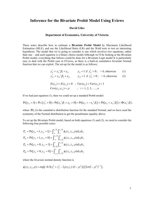
Inference for the Bivariate Probit Model Using Eviews
David Giles
Department of Economics, University of Victoria
These notes describe how to estimate a Bivariate Probit Model by Maximum Likelihood
Estimation (MLE), and use the Likelihood Ratio (LR) and the Wald tests to test an interesting
hypothesis. The model that we’re going to consider is one which involves two equations, rather
than one – and each equation is a binary choice model.Although we’ll be looking at the Bivariate
Probit model, everything that follows could be done for a Bivariate Logit model It is particularly
easy to deal with the Probit case in EViews, as there is a built-in cumulative bivariate Normal
function that we can exploit. The set-up for the model is as follows:
*
yi1 xi1'
1 i1
1 1
*
y i if y i1
0 ; = 0, otherwise (1)
*
y x y
*
1 if y 0 ; = 0, otherwise (2)
i2
i2
' 2 i2
2 i
i2
E( i1)
E(
i
2)
0 ; Var( i1)
Var(
i
2)
1
Cov , ) ; i = 1, 2, 3, …., n
( i1
i2
If we had just equation (1), then we could set up a standard Probit model:
*
Pr[ yi1 1]
Pr.[
yi1
0]
Pr[ xi1'
1 i1
0]
Pr[ i1
xi1'
1]
Pr[ i1
xi1'
1]
(
xi1'
1)
where (.) is the cumulative distribution function for the standard Normal, and we have used the
symmetry of the Normal distribution to get the penultimate equality above.
To set up the Bivariate Probit model, based on both equations (1) and (2), we need to consider the
following four possible cases:
P
P
P
P
11
10
01
00
Pr[ y
Pr[ y
i1
Pr[ y
i1
Pr[ y
i1
i1
1,
y
1,
y
0,
0,
i2
i2
y
i2
y
i2
1]
0]
1]
0]
xi1' xi2'2
1
x '
i1
1
( z , z , )
dz dz
2
xi
2 '2
2
xi
2 '2
2
xi1'1
x 1 '
x
1 2 '
i i 2
1
1
2
( z , z , )
dz dz
2
1
2
( z , z , )
dz dz
1
2
( z , z , )
dz dz
where the bivariate normal density function is
2 2
2
2 1/
2
( z , z , )
exp[ 0.
5(
z z 2
z z ) /( 1
)] /[ 2
( 1
) ] .
2
1
2
1
2
1
2
2
1
1
1
1
2
2
2
2
1

Then, the log-likelihood function for the bivariate model can be obtained in the following way:
(i) Define q y 1
and q y 1
i1
2 i1
i2
2 i2
(ii) Define zij xij
'
j and wij qijzij
; j = 1, 2
*
(iii) Define q q
i i1
i2
*
(iv) Then, Pr[ Y y , Y y ] ( w , w , )
n
1 i1
2 i2
2 i1
i2
i
*
(v) log L log ( w , w , )
i1
2
i1
i2
i
The EViews workfile, bivariate probit.wf1, contains data for the variables y1, y2, x1 and x2. The
LOGL object, LOGL01, allows us to estimate a Bivariate Probit model for y1 and y2. See the
READ_ME text object in the EViews workfile for more details.
We can use a Wald test to test the hypothesis that the errors in the two equations of the model are
independent. This amounts to testing H0: ρ = 0 against a 2-sided alternative. In terms of the
EViews code, we need to test if c(5) = 0. The results are in the table titled
Wald_Test_Result_01. In this case, we cannot reject H0, so in fact we would be justified in
estimating 2 separate Probit models (see EQ01 and EQ02 in the EViews workfile).
We can also use an LR test to test the hypothesis that the errors in the two equations of the model
are independent. In this case we need the maximized value of the log-likelihood function from the
bivariate probit model (i.e., the “unrestricted” model), and the maximized value of the loglikelihood
function from the “unrestricted” model. The latter is just the sum of the 2 maximized
log-likelihood values from the two individual probit models. Here, this number is –(32.96773 +
30.44460) = -63.41233. So, the LR test statistic is 2( -63.16293+63.41233 +) = 0.4988. The p-
2
value based on the (asymptotic) ( 1)
distribution is 0.4800, so again, we would not reject the null
hypothesis.
Finally, note that the model could be extended in several interesting ways. For example, suppose
that we hypothesize that the correlation between the errors in the two equations of the model is
proportional to a third variable, x3. In LOGL02 in the EViews workfile, the code for the loglikelihood
function has been altered to allow for this refinement. If we now apply the Wald test to
see if the errors of the two equations are independent we get the results in the text object titled
Wald_Test_Result_02. Note that the p-value has dropped to approximately 7%, which may well
alter our earlier conclusion. Of course, this is only an asymptotically valid test and our sample
size is just n = 50, so we should be cautious.
March, 2010
2