Analyse et Simulation Numérique par Relaxation d ... - EdF R&D
Analyse et Simulation Numérique par Relaxation d ... - EdF R&D
Analyse et Simulation Numérique par Relaxation d ... - EdF R&D

Create successful ePaper yourself
Turn your PDF publications into a flip-book with our unique Google optimized e-Paper software.
Université Pierre <strong>et</strong> Marie Curie Laboratoire Jacques-Louis Lions<br />
Paris 6 UMR 7598<br />
Thèse de Doctorat de<br />
l’Université Pierre <strong>et</strong> Marie Curie<br />
Présentée <strong>et</strong> soutenue publiquement le 26 novembre 2012<br />
pour l’obtention du grade de<br />
Docteur de l’Université Pierre <strong>et</strong> Marie Curie<br />
Spécialité : Mathématiques Appliquées<br />
<strong>par</strong><br />
Khaled Saleh<br />
<strong>Analyse</strong> <strong>et</strong> <strong>Simulation</strong> <strong>Numérique</strong> <strong>par</strong> <strong>Relaxation</strong><br />
d’Écoulements Diphasiques Compressibles<br />
Contribution au Traitement des Phases Évanescentes<br />
Après avis des rapporteurs<br />
M. Thierry Gallouët<br />
M. Roberto Natalini<br />
Devant le jury composé de<br />
M. Grégoire Allaire Examinateur<br />
M. François Bouchut Examinateur<br />
M. Frédéric Coquel Directeur de Thèse<br />
M. Thierry Gallouët Rapporteur<br />
M me Edwige Godlewski Examinateur<br />
M. Jean-Marc Hérard Directeur de Thèse<br />
M. Nicolas Seguin Co-Encadrant<br />
École Doctorale de Sciences Mathématiques de Paris Centre Faculté de Mathématiques<br />
ED 386 UFR 929
Khaled Saleh :<br />
UPMC, Université Paris 06, UMR 7598, Laboratoire Jacques-Louis Lions, F-75005, Paris, France.<br />
CNRS, UMR 7598, Laboratoire Jacques-Louis Lions, F-75005, Paris, France.<br />
EDF R&D, Dé<strong>par</strong>tement Mécanique des Fluides, Energies, Environnement,<br />
6 quai Watier BP 49, 78401 Chatou Cedex, France.<br />
Adresse électronique: saleh@ann.jussieu.fr
Remerciements<br />
Je tiens en premier lieu à remercier mes deux directeurs de thèse, Frédéric Coquel <strong>et</strong> Jean-Marc<br />
Hérard, ainsi que Nicolas Seguin, mon troisième (<strong>et</strong> non le moindre) encadrant. Comme je le dis<br />
souvent, j’ai été, durant ces trois années de thèse, extrêmement bien entouré, puisque j’ai eu la<br />
chance de bénéficier du soutien, de l’expérience <strong>et</strong> des conseils de trois remarquables chercheurs. Ils<br />
ont été, tout au long de ces trois années, toujours disponibles <strong>et</strong> je les salue tous les trois pour leurs<br />
remarquables qualités pédagogiques. Il est rare, je pense, d’être entouré d’aussi bons professeurs,<br />
qui ont toujours su répondre avec clarté <strong>et</strong> précision à mes interrogations. Je salue aussi leur grande<br />
gentillesse <strong>et</strong> leurs conseils avisés, qui m’ont aidé à orienter mon choix de carrière. Merci à Frédéric<br />
pour sa persévérance <strong>et</strong> son optimisme à toute épreuve, me poussant toujours à aller jusqu’au bout<br />
des résultats, même ceux qui étaient difficiles à démontrer. Je le remercie aussi pour sa minutie dans<br />
la relecture, qui a grandement contribué à améliorer mes écrits ! D’ailleurs, je crois que cela a été<br />
contagieux, puisque je suis moi même devenu très (trop ?) perfectionniste... Merci à Jean-Marc, qui<br />
a toujours su replacer mes recherches dans leur contexte industriel. J’ai appris grâce à lui qu’il était<br />
possible de concilier mon goût pour les mathématiques <strong>et</strong> les préoccupations industrielles comme<br />
celles d’un grand groupe comme EDF. Merci enfin à Nicolas pour sa disponibilité, sa pédagogie <strong>et</strong><br />
sa rigueur. Merci pour toutes les fois où je n’arrivais pas à débugger mon code! Par ailleurs, je<br />
serai toujours admiratif de son impressionnant sens physique.<br />
Je remercie Thierry Gallouët <strong>et</strong> Roberto Natalini d’avoir accepté de rapporter sur ce manuscrit.<br />
Je remercie en <strong>par</strong>ticulier Thierry pour les échanges très intéressants que nous avons pu avoir,<br />
concernant mes travaux. Je remercie également Grégoire Allaire d’avoir accepté de faire <strong>par</strong>tie<br />
de mon jury de soutenance, <strong>et</strong> de l’avoir présidé. J’ai été également très heureux de compter<br />
<strong>par</strong>mi les membres de mon jury François Bouchut <strong>et</strong> Edwige Godlewski. Merci aussi à Sergey<br />
Gavrilyuk d’avoir accepté de <strong>par</strong>ticiper à mon jury, même s’il n’a pas pu être présent pour des<br />
raisons indépendantes de sa volonté.<br />
Ce travail a été réalisé au sein du dé<strong>par</strong>tement Mécanique des Fluides, Energies, Environnement,<br />
de la division Recherche <strong>et</strong> Développement d’EDF. Je souhaite à ce titre remercier EDF <strong>et</strong> l’ANRT<br />
pour le financement du contrat CIFRE, dont j’ai bénéficié durant ces trois années de recherche. A<br />
EDF, j’ai eu le plaisir de faire <strong>par</strong>tie du groupe I81 au dé<strong>par</strong>tement MFEE. Je voudrais remercier<br />
Isabelle Flour, chef du groupe I81 pendant mon séjour à EDF. Elle est à mes yeux l’exemple même<br />
du chef rigoureux <strong>et</strong> proche à la fois. Je la remercie de s’être toujours assurée du bon déroulement de<br />
ma thèse au sein du groupe. Merci aux thésards du groupe qui contribuent grandement à l’excellente<br />
ambiance qui règne à Chatou. Merci aux anciens : La<strong>et</strong>itia, Bertrand <strong>et</strong> Arnaud (ton accent te<br />
perdra). Merci à Clara <strong>et</strong> Sana pour votre constante bonne humeur (<strong>et</strong> aussi pour la douce musique<br />
3
de vos talons hauts que j’ai appris à reconnaître à des dizaines de mètres !). Je pense également à<br />
Avner <strong>et</strong> Romain, toujours <strong>par</strong>tants pour résoudre un exo de maths, à Christophe (tes pâtisseries me<br />
manquent déjà), ainsi qu’à Franck. Merci enfin à ma grande sœur de thèse Kateryna pour ces trois<br />
années de bonne humeur. Merci à toi pour ta gentillesse incommensurable <strong>et</strong> un grand merci d’avoir<br />
été mon agent <strong>et</strong> d’avoir fait ma pub auprès de qui tu sais ! Je n’oublie pas non plus les stagiaires<br />
que j’ai croisés au dé<strong>par</strong>tement : Marie l’antiboise, Erwan (pro du ping-pong), Vincent (toujours<br />
dernier à sortir de table) <strong>et</strong> aussi une jeune stagiaire prénommée Haïfa, dont je me demande ce<br />
qu’elle est devenue. Je souhaite aussi remercier les ingénieurs d’EDF avec qui j’ai pu échanger,<br />
voire travailler lors de c<strong>et</strong>te thèse : Olivier Hurisse, Bruno Audebert, Jérôme Lavieville, Frédéric<br />
Archambeau, Martin Ferrand, Mathieu Guingo. Merci enfin à Marie-Line, Chantal <strong>et</strong> Eliane pour<br />
leur accueil chaleureux à l’antenne de gestion du groupe.<br />
Une autre grande chance pour moi a été de faire <strong>par</strong>tie intégrante des doctorants du laboratoire<br />
Jacques-Louis Lions, ce qui n’était pas a priori évident pour un doctorant en entreprise. J’y ai<br />
développé de nombreux contacts à la fois sur le plan professionnel <strong>et</strong> sur le plan humain. Je souhaite<br />
exprimer ma gratitude à Edwige Godlewski, directrice adjointe du laboratoire <strong>et</strong> Yvon Maday,<br />
directeur du laboratoire, qui se sont assurés que mon séjour au laboratoire se déroule dans les<br />
meilleures conditions, notamment après la fin de mon contrat avec EDF. Merci aussi au secrétariat<br />
du laboratoire : Mesdames Boulic <strong>et</strong> Ruprecht, Madame Lendo <strong>et</strong> Madame Foucart <strong>et</strong> bien sûr<br />
Madame Salima Lounici. Je voudrais aussi remercier Khashayar Dadras <strong>et</strong> saluer l’excellent travail<br />
qu’il accomplit pour le bon fontionnement de l’informatique au laboratoire. Merci également à<br />
Christian David, grâce à qui j’ai toujours eu le matériel dont j’avais besoin. Merci enfin à Antoine<br />
Le Hyaric pour l’aide qu’il m’a apportée sur mes videos de simulations numériques. Passer du temps<br />
au laboratoire a toujours été pour moi un plaisir, grâce notamment aux doctorants du bureau 15-25<br />
302 : Kamel, un ami valeureux <strong>et</strong> mon témoin de mariage, Imen, Etienne, Kirill, Pierre, Pierre-<br />
Henri, <strong>et</strong> enfin Simona, Luis-Miguel <strong>et</strong> Abdellah, avec qui nous aurions pu ouvrir une p<strong>et</strong>ite cafétéria<br />
dans le bureau ! Il y a aussi les autres doctorants du laboratoire : Lise-Marie, Charles (j’aurais aimé<br />
lire ce que tu fais mais c’est écrit trop p<strong>et</strong>it), Hassan, Haidar, Magali, les « contrôleurs » Malik <strong>et</strong><br />
Vincent. Merci aux organisateurs du GTT, qui ont toujours su m’avoir <strong>par</strong> les sentiments. Ayant<br />
chaque semaine la ferme intention de faire le pique-assi<strong>et</strong>te au goûter du GTT avant de directement<br />
re<strong>par</strong>tir travailler, je suis toujours (ok presque toujours) resté pour l’exposé, <strong>et</strong> j’ai pu y voir des<br />
exposés de très grande qualité, dont certains, je l’avoue, me faisaient un peu complexer... Merci<br />
donc à Alexis, Nicole, Juli<strong>et</strong>te <strong>et</strong> Jean-Paul. Jean-Paul, qui même après huit heures de vol <strong>et</strong> un<br />
décalage horaire, a réussi à débloquer une difficulté sur laquelle je bloquais depuis pas mal de temps.<br />
Merci encore pour cela ! Je pense également à Benjamin, mon grand frère de thèse, que je remercie<br />
pour ses conseils avisés. Je me souviendrai toujours de l’ambiance exceptionnelle qui régnait dans<br />
le voisinage du bureau 16-26 301, grâce aux jeunes chercheurs permanents ou de passage : Nicolas<br />
<strong>et</strong> Nicolas (qui se dé<strong>par</strong>tageront), Laurent <strong>et</strong> Jean-François bien sûr, mais aussi Fred (Lagoutière)<br />
<strong>et</strong> Fred (Charles), Clément, Franck <strong>et</strong> l’autre membre de l’ « Egyptian connection » : Ayman.<br />
Merci aussi à Christophe Chalons avec qui j’ai toujours eu plaisir de discuter Baer-Nunziato <strong>et</strong> à<br />
Emmanuel Audusse avec qui j’ai apprécié travailler (d’ailleurs ce n’est pas fini, il faut vraiment<br />
qu’on termine ce papier, n’est-ce pas Nicolas ?).<br />
Le CEMRACS 2011 a été pour moi une très agréable expérience. Il m’a permis d’avancer sur<br />
ma thèse, en <strong>par</strong>ticulier sur le quatrième chapitre, tout en ayant l’impression d’être en vacances<br />
(mais j’ai quand même bossé hein !). J’ai d’excellents souvenirs avec Anne-Céline (« pourquoi, y’a<br />
deux Célines ? »), Anne-Claire, Guilhem <strong>et</strong> Benoit, mais aussi avec la « team ramadan » : Tassadit<br />
4
(à qui je souhaite une excellente fin de thèse sur Baer-Nunziato !), El Hassan, Mohamed Abaidi («<br />
pourquoi, y’a deux Célines ? ») <strong>et</strong> Mohamed Ghattassi. Merci aussi à Nina, Mathieu, Rémi, David<br />
<strong>et</strong> Fabien, pour n’avoir jamais voulu m’apprendre la Quinche... Merci enfin aux strasbourgeois,<br />
Anaïs, Hélène, <strong>et</strong> les garçons : Jonathan <strong>et</strong> Ahmed. Ahmed, qui m’a appris, à moi l’Egyptien,<br />
comment pré<strong>par</strong>er une chicha.<br />
Merci à Mohamed Jaoua de m’avoir permis d’enseigner à l’Université Française d’Egypte. Merci<br />
aussi à Manuel pour ses excellents plans resto au Caire !<br />
Avant de commencer c<strong>et</strong>te thèse, j’ai eu le plaisir de suivre les cours du master ANEDP de Paris<br />
6, où j’ai fait la connaissance de jeunes chercheurs d’horizons très différents, devenus pour certains<br />
des amis. Je pense à Nafi, Maxime, Cécile, Manu, Morgan <strong>et</strong> Aurore, <strong>et</strong> je souhaite bon courage à<br />
ceux d’entre eux qui finissent bientôt leur thèse.<br />
Je remercie également mes meilleurs amis, Wassef, Ali <strong>et</strong> Sullym (dans l’ordre chronologique de<br />
rencontre). Je crois que je ne compte plus les fous rires qu’on a pu avoir ensemble ! Merci à vous<br />
trois d’avoir été là <strong>et</strong> de m’avoir permis, chacun à sa façon, de sortir un p<strong>et</strong>it peu de mon univers<br />
de matheux.<br />
Un grand MERCI à ma famille, en France <strong>et</strong> en Egypte, pour m’avoir soutenu durant toutes<br />
mes années d’études. Merci à mes frères Nouredine <strong>et</strong> Nassim (les lascars, experts de la vanne)<br />
d’avoir manqué vos cours pour assister à ma soutenance. Bon courage pour vos études, <strong>et</strong> si jamais<br />
vous avez des questions, on va voir ce qu’on peut faire. Merci à ma sœur Ghadah ainsi qu’à son<br />
époux Mohamed, <strong>et</strong> bienvenue à mon p<strong>et</strong>it neveu Adam (plus tard, tu pourras dire que j’ai <strong>par</strong>lé de<br />
toi dans ma thèse). Et surtout, surtout, merci à mes <strong>par</strong>ents, que j’aime tendrement. Merci pour<br />
tous les sacrifices que vous avez faits <strong>et</strong> continuez de faire pour nous. Que Dieu vous garde à nos<br />
côtés.<br />
Enfin, je dédie ce travail à ma très chère femme Haïfa. Merci pour ton amour, ta tendresse, ton<br />
amitié, ton soutien dans les moments difficiles. Toi qui as toujours su m’encourager <strong>et</strong> me donner<br />
confiance en moi, merci d’être là. Tout ceci n’est rien sans toi.<br />
5
Résumé<br />
Dans le cadre du nucléaire civil, la modélisation des écoulements diphasiques est nécessaire à la<br />
représentation de nombreuses configurations d’écoulements fluides dans les circuits primaire <strong>et</strong><br />
secondaire des centrales s’appuyant sur des réacteurs à eau pressurisée (REP). Les applications<br />
visées concernent non seulement le fonctionnement nominal, mais aussi <strong>et</strong> surtout les configurations<br />
incidentelles, <strong>par</strong>mi lesquelles on peut citer l’accident <strong>par</strong> perte de réfrigérant primaire (APRP),<br />
les phénomènes de crise d’ébullition, mais aussi le renoyage des coeurs. En régime nominal dans<br />
le circuit primaire, le fonctionnement est très proche du fonctionnement monophasique pur, la<br />
vapeur étant a priori absente. En revanche, le taux de présence de vapeur peut devenir de faible à<br />
conséquent dans les situations incidentelles.<br />
C<strong>et</strong>te thèse s’intéresse plus <strong>par</strong>ticulièrement au modèle diphasique de Baer-Nunziato qui entre<br />
dans la classe des modèles bifluides hyperboliques. L’objectif de ce travail est de proposer quelques<br />
techniques de prise en compte de la dis<strong>par</strong>ition de phase, régime qui occasionne d’importantes<br />
instabilités tant au niveau du modèle qu’au niveau de sa simulation numérique.<br />
L’enseignement principal de la thèse est que dans ces régimes, il est possible des stabiliser<br />
les solutions en introduisant une dissipation de l’entropie totale de mélange. D’un point de vue<br />
numérique, c<strong>et</strong>te dissipation d’entropie supplémentaire perm<strong>et</strong> en eff<strong>et</strong> d’obtenir des approximations<br />
stables dans ces régimes. Les méthodes d’analyse <strong>et</strong> d’approximation proposées reposent de<br />
façon intensive sur les techniques d’approximation <strong>par</strong> relaxation de type Suliciu, <strong>et</strong> les méthodes<br />
numériques qui en découlent. Deux approches sont principalement étudiées.<br />
Dans une première approche dite approche Eulerienne directe, la résolution exacte du problème<br />
de Riemann pour le système relaxé perm<strong>et</strong> de définir un schéma numérique extrêmement précis<br />
pour le modèle de Baer-Nunziato. Nous montrons que dans les régimes de fonctionnement normal<br />
(i.e. sans dis<strong>par</strong>ition de phase), la méthode numérique ainsi obtenue est bien plus économique en<br />
terme de coût CPU (à précision donnée) que le schéma classique très simple de Rusanov. De plus,<br />
nous montrons que ce nouveau schéma est très robuste puisqu’il perm<strong>et</strong> la simulation des régimes de<br />
dis<strong>par</strong>ition de phase. Les travaux furent initialement développés sur la version 1D du modèle, pour<br />
laquelle une inégalité d’entropie discrète vérifiée <strong>par</strong> le schéma fut démontrée. Ils furent ensuite<br />
étendus en 3D <strong>et</strong> intégrés à un prototype de code industriel développé <strong>par</strong> EDF.<br />
La deuxième approche, dite approche <strong>par</strong> splitting acoustique, propose à travers un opérateur de<br />
splitting temporel, de sé<strong>par</strong>er les phénomènes de propagation d’ondes acoustiques <strong>et</strong> les phénomènes<br />
associés au transport matériel. C<strong>et</strong>te approche a le double objectif d’éviter la résonance due à<br />
7
l’interaction entre ces deux types d’ondes, mais surtout de perm<strong>et</strong>tre à long terme un traitement<br />
implicite des phénomènes acoustiques, tout en explicitant la discrétisation des phénomènes de transport.<br />
On <strong>par</strong>le alors de méthodes semi-implicites. Le schéma que nous proposons adm<strong>et</strong> une mise<br />
en oeuvre remarquablement simple. De plus, nous montrons qu’il perm<strong>et</strong> la prise en compte simple<br />
de la dis<strong>par</strong>ition de phase. Une des principales nouveautés de ce travail est d’exploiter des<br />
ferm<strong>et</strong>ures dissipatives du couple vitesse <strong>et</strong> pression d’interface, <strong>et</strong> de montrer que ces ferm<strong>et</strong>ures<br />
perm<strong>et</strong>tent le contrôle de la taille des solutions du problème de Riemann associé à l’étape acoustique.<br />
8
Abstract<br />
This thesis deals with the Baer-Nunziato two-phase flow model. The main objective of this work is<br />
to propose some techniques to cope with phase vanishing regimes which produce important instabilities<br />
in the model and its numerical simulations. Through analysis and simulation m<strong>et</strong>hods using<br />
Suliciu relaxation approximations, we prove that in these regimes, the solutions can be stabilised<br />
by introducing some extra dissipation of the total mixture entropy.<br />
In a first approach, called the Eulerian approach, the exact resolution of the relaxation Riemann<br />
problem provides an accurate entropy-satisfying numerical scheme, which turns out to be much more<br />
efficient in terms of CPU-cost than the classical and very simple Rusanov’s scheme. Moreover, the<br />
scheme is proved to handle the vanishing phase regimes with great stability. The scheme, first<br />
developed in 1D, is then extended in 3D and implemented in an industrial code developed by EDF.<br />
The second approach, called the acoustic splitting approach, considers a se<strong>par</strong>ation of fast<br />
acoustic waves from slow material waves. The objective is to avoid the resonance due to the<br />
interaction b<strong>et</strong>ween these two types of waves, and to allow an implicit treatment of the acoustics,<br />
while material waves are explicitly discr<strong>et</strong>ized. The resulting scheme is very simple and allows to<br />
deal simply with phase vanishing. The originality of this work is to use new dissipative closure laws<br />
for the interfacial velocity and pressure, in order to control the solutions of the Riemann problem<br />
associated with the acoustic step, in the phase vanishing regimes.<br />
9
Table des matières<br />
Remerciements 3<br />
Résumé 7<br />
Abstract 9<br />
Introduction générale 17<br />
0.1 Contexte général . . . . . . . . . . . . . . . . . . . . . . . . . . . . . . . . . . . . . . 18<br />
0.2 Les modèles diphasiques de type Baer-Nunziato . . . . . . . . . . . . . . . . . . . . . 20<br />
0.2.1 Le modèle avec énergie en plusieurs variables d’espace . . . . . . . . . . . . . 20<br />
0.2.2 Le modèle avec énergie en une dimension d’espace . . . . . . . . . . . . . . . 22<br />
0.2.3 Le modèle barotrope en une dimension d’espace . . . . . . . . . . . . . . . . . 23<br />
0.3 Produits non conservatifs, entropie <strong>et</strong> résonance . . . . . . . . . . . . . . . . . . . . . 24<br />
0.4 Approximation <strong>par</strong> relaxation <strong>et</strong> passage du barotrope à l’énergie . . . . . . . . . . . 27<br />
0.5 Chapitre 1: Approximation <strong>par</strong> relaxation pour les équations d’Euler en tuyère . . . 27<br />
0.6 Chapitre 2: Approximation <strong>par</strong> relaxation pour le modèle de Baer-Nunziato . . . . . 29<br />
0.7 Chapitre 3: Un schéma numérique de relaxation pour le modèle de Baer-Nunziato . 31<br />
0.8 Chapitre 4: Une méthode à pas fractionnaires pour le modèle de Baer-Nunziato . . . 33<br />
0.9 Publications . . . . . . . . . . . . . . . . . . . . . . . . . . . . . . . . . . . . . . . . . 36<br />
Bibliographie . . . . . . . . . . . . . . . . . . . . . . . . . . . . . . . . . . . . . . . . . . . 38<br />
1 Approximation <strong>par</strong> relaxation pour les équations d’Euler en tuyère 41<br />
1.1 Introduction . . . . . . . . . . . . . . . . . . . . . . . . . . . . . . . . . . . . . . . . . 42<br />
11
1.2 The Euler equations in a nozzle with variable cross-section . . . . . . . . . . . . . . . 44<br />
1.2.1 Presentation and main properties . . . . . . . . . . . . . . . . . . . . . . . . . 44<br />
1.2.2 Standing wave and resonance . . . . . . . . . . . . . . . . . . . . . . . . . . . 45<br />
1.2.3 Numerical approximation and Riemann solvers . . . . . . . . . . . . . . . . . 46<br />
1.3 <strong>Relaxation</strong> approximation . . . . . . . . . . . . . . . . . . . . . . . . . . . . . . . . . 46<br />
1.3.1 The relaxation system and its main properties . . . . . . . . . . . . . . . . . 46<br />
1.3.2 Jump relations across the stationary contact discontinuity . . . . . . . . . . . 48<br />
1.3.3 Solving the Riemann problem for the relaxation system . . . . . . . . . . . . 49<br />
1.4 Numerical approximation . . . . . . . . . . . . . . . . . . . . . . . . . . . . . . . . . 65<br />
1.4.1 The relaxation m<strong>et</strong>hod . . . . . . . . . . . . . . . . . . . . . . . . . . . . . . . 65<br />
1.4.2 Finite volume formulation . . . . . . . . . . . . . . . . . . . . . . . . . . . . . 67<br />
1.4.3 Basic properties of the scheme . . . . . . . . . . . . . . . . . . . . . . . . . . 68<br />
1.4.4 Non linear stability . . . . . . . . . . . . . . . . . . . . . . . . . . . . . . . . . 70<br />
1.4.5 Practical choice of the <strong>par</strong>am<strong>et</strong>er a . . . . . . . . . . . . . . . . . . . . . . . . 82<br />
1.4.6 Numerical results . . . . . . . . . . . . . . . . . . . . . . . . . . . . . . . . . . 84<br />
Appendices . . . . . . . . . . . . . . . . . . . . . . . . . . . . . . . . . . . . . . . . . . . . 86<br />
References . . . . . . . . . . . . . . . . . . . . . . . . . . . . . . . . . . . . . . . . . . . . . 88<br />
2 Approximation <strong>par</strong> relaxation pour le modèle de Baer-Nunziato 93<br />
2.1 Introduction . . . . . . . . . . . . . . . . . . . . . . . . . . . . . . . . . . . . . . . . . 94<br />
2.1.1 The isentropic model of Baer-Nunziato . . . . . . . . . . . . . . . . . . . . . . 95<br />
2.1.2 A relaxation approximation . . . . . . . . . . . . . . . . . . . . . . . . . . . . 97<br />
2.2 The Riemann problem for the relaxation system . . . . . . . . . . . . . . . . . . . . 98<br />
2.2.1 Definition of the solutions to the Riemann problem . . . . . . . . . . . . . . . 99<br />
2.2.2 The resolution strategy: an iterative procedure . . . . . . . . . . . . . . . . . 102<br />
2.2.3 An existence theorem for solutions with subsonic wave ordering . . . . . . . . 106<br />
2.2.4 The Riemann problem for phase 2 with a predicted value of π ∗ 1 . . . . . . . . 108<br />
2.2.5 The Riemann problem for phase 1 with a predicted value of u ∗ 2 . . . . . . . . 110<br />
2.2.6 Solution of the fixed point problem and proof of Theorem 2.2.3 . . . . . . . 116<br />
2.2.7 Expression of the Riemann solution . . . . . . . . . . . . . . . . . . . . . . . 121<br />
12
References . . . . . . . . . . . . . . . . . . . . . . . . . . . . . . . . . . . . . . . . . . . . . 122<br />
3 Un schéma numérique de relaxation pour le modèle de Baer-Nunziato 125<br />
3.1 Introduction . . . . . . . . . . . . . . . . . . . . . . . . . . . . . . . . . . . . . . . . . 126<br />
3.2 The model and its relaxation approximation . . . . . . . . . . . . . . . . . . . . . . . 128<br />
3.3 The relaxation Riemann solver . . . . . . . . . . . . . . . . . . . . . . . . . . . . . . 130<br />
3.3.1 An existence theorem for subsonic solutions . . . . . . . . . . . . . . . . . . . 130<br />
3.3.2 Construction of the solution . . . . . . . . . . . . . . . . . . . . . . . . . . . . 132<br />
3.4 The relaxation scheme . . . . . . . . . . . . . . . . . . . . . . . . . . . . . . . . . . . 136<br />
3.4.1 Description of the relaxation algorithm . . . . . . . . . . . . . . . . . . . . . . 136<br />
3.4.2 Finite volume formulation . . . . . . . . . . . . . . . . . . . . . . . . . . . . . 137<br />
3.4.3 Basic properties of the scheme . . . . . . . . . . . . . . . . . . . . . . . . . . 138<br />
3.4.4 Non-linear stability . . . . . . . . . . . . . . . . . . . . . . . . . . . . . . . . . 139<br />
3.4.5 Practical choice of the pair (a1, a2) . . . . . . . . . . . . . . . . . . . . . . . . 143<br />
3.5 Numerical tests for the barotropic 1D model . . . . . . . . . . . . . . . . . . . . . . . 144<br />
3.5.1 Test-case 1: a compl<strong>et</strong>e Riemann problem . . . . . . . . . . . . . . . . . . . . 145<br />
3.5.2 Test-case 2: a vanishing phase case . . . . . . . . . . . . . . . . . . . . . . . . 146<br />
3.5.3 Test-case 3: Coupling b<strong>et</strong>ween two pure phases . . . . . . . . . . . . . . . . . 147<br />
3.6 The multidimensional case . . . . . . . . . . . . . . . . . . . . . . . . . . . . . . . . . 148<br />
3.6.1 The two-dimensionnal finite volume scheme . . . . . . . . . . . . . . . . . . . 149<br />
3.6.2 Numerical approximation of the source terms . . . . . . . . . . . . . . . . . . 151<br />
3.6.3 Numerical illustration . . . . . . . . . . . . . . . . . . . . . . . . . . . . . . . 153<br />
3.7 Extension to the full Baer-Nunziato model in 1D . . . . . . . . . . . . . . . . . . . . 153<br />
3.7.1 Entropy-Energy duality for the Euler equations . . . . . . . . . . . . . . . . . 155<br />
3.7.2 Extension to the Baer-Nunziato equations . . . . . . . . . . . . . . . . . . . . 158<br />
3.7.3 The fixed point procedure . . . . . . . . . . . . . . . . . . . . . . . . . . . . . 161<br />
3.7.4 Numerical illustration . . . . . . . . . . . . . . . . . . . . . . . . . . . . . . . 168<br />
Appendices . . . . . . . . . . . . . . . . . . . . . . . . . . . . . . . . . . . . . . . . . . . . 168<br />
References . . . . . . . . . . . . . . . . . . . . . . . . . . . . . . . . . . . . . . . . . . . . . 172<br />
13
4 Une méthode à pas fractionnaires pour le modèle de Baer-Nunziato 181<br />
4.1 The isentropic Baer-Nunziato model . . . . . . . . . . . . . . . . . . . . . . . . . . . 182<br />
4.1.1 Classical Closure laws for the pair (VI, PI) . . . . . . . . . . . . . . . . . . . . 183<br />
4.1.2 Closure laws for S(U) and stabilization effects . . . . . . . . . . . . . . . . . . 184<br />
4.1.3 Dissipative correction of the closure laws (VI, PI) . . . . . . . . . . . . . . . . 185<br />
4.2 An operator splitting m<strong>et</strong>hod for the Baer-Nunziato model . . . . . . . . . . . . . . 186<br />
4.3 Analysis and numerical treatment of the first step . . . . . . . . . . . . . . . . . . . 189<br />
4.3.1 A relaxation approximation . . . . . . . . . . . . . . . . . . . . . . . . . . . . 189<br />
4.3.2 Dissipative closure laws for (VI, ΠI) . . . . . . . . . . . . . . . . . . . . . . . 190<br />
4.3.3 Jump relations for the Riemann problem . . . . . . . . . . . . . . . . . . . . 192<br />
4.3.4 Boundedness of the solution in the regime of vanishing phases . . . . . . . . . 193<br />
4.3.5 Numerical approximation of the first step . . . . . . . . . . . . . . . . . . . . 199<br />
4.4 Numerical approximation of the second step . . . . . . . . . . . . . . . . . . . . . . . 202<br />
4.5 Numerical approximation of the third step . . . . . . . . . . . . . . . . . . . . . . . . 204<br />
4.6 Global conservativity of the scheme . . . . . . . . . . . . . . . . . . . . . . . . . . . . 205<br />
4.7 Extension of the scheme to the model with energies . . . . . . . . . . . . . . . . . . . 209<br />
4.8 Numerical applications . . . . . . . . . . . . . . . . . . . . . . . . . . . . . . . . . . . 209<br />
4.8.1 The isentropic case . . . . . . . . . . . . . . . . . . . . . . . . . . . . . . . . . 209<br />
4.8.2 Compl<strong>et</strong>e model with energies . . . . . . . . . . . . . . . . . . . . . . . . . . . 210<br />
Appendices . . . . . . . . . . . . . . . . . . . . . . . . . . . . . . . . . . . . . . . . . . . . 211<br />
References . . . . . . . . . . . . . . . . . . . . . . . . . . . . . . . . . . . . . . . . . . . . . 218<br />
Annexes 225<br />
A Convexité de l’entropie mathématique pour le modèle de Baer-Nunziato 225<br />
B Un schéma à pas fractionnaires simple pour le modèle de Baer-Nunziato 229<br />
B.1 The Baer-Nunziato two-phase flow model and its mathematical properties . . . . . . 231<br />
B.2 A Splitting m<strong>et</strong>hod for the Baer-Nunziato model . . . . . . . . . . . . . . . . . . . . 233<br />
B.2.1 Numerical approximation . . . . . . . . . . . . . . . . . . . . . . . . . . . . . 233<br />
14
B.2.2 Treatment of the first step . . . . . . . . . . . . . . . . . . . . . . . . . . . . . 234<br />
B.2.3 Treatment of the second step . . . . . . . . . . . . . . . . . . . . . . . . . . . 239<br />
B.3 Numerical experiments . . . . . . . . . . . . . . . . . . . . . . . . . . . . . . . . . . . 242<br />
B.3.1 Test case 1: a contact discontinuity . . . . . . . . . . . . . . . . . . . . . . . . 243<br />
B.3.2 Test case 2: a compl<strong>et</strong>e case with all the waves . . . . . . . . . . . . . . . . . 243<br />
B.4 Conclusion . . . . . . . . . . . . . . . . . . . . . . . . . . . . . . . . . . . . . . . . . 244<br />
References . . . . . . . . . . . . . . . . . . . . . . . . . . . . . . . . . . . . . . . . . . . . . 246<br />
C Un modèle de type Baer-Nunziato avec ferm<strong>et</strong>ures dynamiques des quantités<br />
interfaciales 251<br />
C.1 Introduction . . . . . . . . . . . . . . . . . . . . . . . . . . . . . . . . . . . . . . . . . 252<br />
C.2 Governing s<strong>et</strong> of equations of the two-fluid model . . . . . . . . . . . . . . . . . . . . 254<br />
C.2.1 Closure laws for Pi and interfacial transfer terms . . . . . . . . . . . . . . . . 255<br />
C.2.2 Closure laws for Vi and W . . . . . . . . . . . . . . . . . . . . . . . . . . . . . 256<br />
C.3 Main properties of the two-fluid model . . . . . . . . . . . . . . . . . . . . . . . . . . 256<br />
C.4 Numerical experiments . . . . . . . . . . . . . . . . . . . . . . . . . . . . . . . . . . . 258<br />
References . . . . . . . . . . . . . . . . . . . . . . . . . . . . . . . . . . . . . . . . . . . . . 260<br />
15
Introduction générale<br />
17
0.1 Contexte général<br />
La modélisation des écoulements diphasiques est nécessaire à la représentation de nombreuses configurations<br />
d’écoulements fluides <strong>et</strong>, si l’on se restreint au cadre nucléaire civil, devient essentielle<br />
dans le contexte des écoulements dans les circuits primaire <strong>et</strong> secondaire des centrales s’appuyant<br />
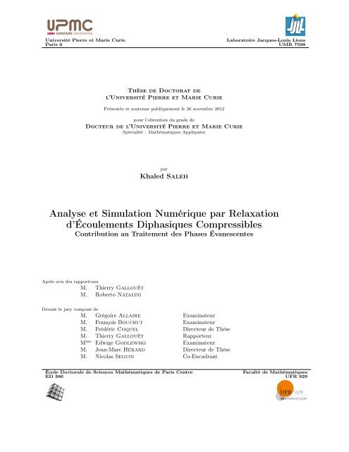
sur des réacteurs à eau pressurisée (REP) (pour une représentation schématique d’une centrale de<br />
type REP, voir la figure 0.1). Ceci justifie l’intérêt constant porté <strong>par</strong> EDF, le CEA <strong>et</strong> l’IRSN<br />
depuis de nombreuses années à ce domaine. Les applications visées concernent non seulement le<br />
fonctionnement nominal, mais aussi <strong>et</strong> surtout les configurations incidentelles, <strong>par</strong>mi lesquelles on<br />
peut citer l’accident <strong>par</strong> perte de réfrigérant primaire (APRP), les phénomènes de crise d’ébullition,<br />
mais aussi le renoyage des cœurs. Le fonctionnement des générateurs de vapeur <strong>et</strong> des condenseurs<br />
constitue un autre champ d’application de c<strong>et</strong>te classe de modèles fluides.<br />
Dans c<strong>et</strong>te optique, les acteurs mentionnés précédemment mais aussi AREVA développent conjointement,<br />
au sein du proj<strong>et</strong> NEPTUNE, une plateforme de codes de simulation des écoulements<br />
diphasiques, ayant pour objectif de fournir des approximations discrètes des solutions de plusieurs<br />
modèles diphasiques, <strong>et</strong> autorisant le couplage de ces codes ([26]). En régime nominal dans le circuit<br />
primaire, le fonctionnement est très proche du fonctionnement monophasique pur, la vapeur étant<br />
a priori absente. En revanche, le taux de présence de vapeur peut devenir de faible à conséquent<br />
dans les situations incidentelles. Dans ce cas, les inhomogénéités spatiales <strong>et</strong> temporelles deviennent<br />
importantes, <strong>et</strong> il convient alors, si l’on souhaite associer un caractère prédictif aux simulations,<br />
disposer de modèles conduisant a minima à des problèmes de Cauchy bien posés.<br />
Deux grandes classes de modèles moyennés, (i.e. proposant des équations d’évolution pour les<br />
moments statistiques d’ordre un au moins) ont été proposées dans la littérature depuis les années<br />
1970 (voir <strong>par</strong>mi d’autres références les ouvrages [29, 21]). Une première classe correspond à une<br />
représentation homogène monofluide, décrivant essentiellement les propriétés moyennes du mélange<br />
eau-vapeur (masse, débit, énergie), <strong>et</strong> éventuellement le déséquilibre de titre masse. Les codes<br />
français THYC (EDF), FLICA <strong>et</strong> GENEPI (CEA), sont basés sur de tels modèles d’écoulements<br />
diphasiques. Une autre approche possible repose sur l’utilisation de l’approche à deux fluides,<br />
c’est le cas pour les codes CATHARE <strong>et</strong> NEPTUNE_CFD (France) <strong>et</strong> RELAP (USA). Dans c<strong>et</strong>te<br />
dernière formulation, les moments d’ordre un associés à la densité, au débit, <strong>et</strong> à l’énergie sont<br />
prédits <strong>par</strong> des lois d’évolution pour chaque phase, le taux de présence statistique de phase étant<br />
fourni <strong>par</strong> une équation d’évolution ou une ferm<strong>et</strong>ure algébrique. L’approche monofluide perm<strong>et</strong><br />
d’éviter le recours à de nombreuses lois de ferm<strong>et</strong>ure, hormis sur le plan des lois d’état thermodynamique<br />
<strong>et</strong> des transferts de masse interfaciaux. Les systèmes fermés associés ont en général une<br />
structure convective assez proche de celle des équations d’Euler, <strong>et</strong> l’on peut dans certains cas (les<br />
plus simples) s’appuyer sur des résultats de caractérisation des solutions de ces équations. Un inconvénient<br />
évident est qu’ils ne fournissent pas d’information précise <strong>et</strong> pertinente sur les déséquilibres<br />
de vitesse/pression/température entre phases. Enfin, dans les cas optimaux, l’obtention de solutions<br />
numériques raisonnablement proches de la convergence ne requiert pas obligatoirement des<br />
maillages très fins. Inversement, l’approche à deux fluides fournit a priori une représentation plus<br />
fine de la réalité en prenant en compte les déséquilibres entre phases, mais elle nécessite de fournir<br />
des lois de ferm<strong>et</strong>ure cohérentes (notamment <strong>par</strong> rapport à la caractérisation entropique) <strong>et</strong> suf-<br />
18
fisamment renseignées (pour ce qui concerne les échelles de temps de relaxation <strong>par</strong> exemple). En<br />
outre, il n’existe pas de consensus actuellement concernant la forme optimale des lois de ferm<strong>et</strong>ure<br />
des termes de transfert interfacial, ou des échelles de temps de relaxation. Selon que l’on considère<br />
telle ou telle loi de ferm<strong>et</strong>ure, les propriétés des modèles peuvent clairement différer. Au-delà de<br />
la difficulté du traitement des phases évanescentes, problème sur lequel tout le monde s’accorde,<br />
des discussions perdurent sur la nature hyperbolique du système au premier ordre. Ce système<br />
s’écrivant sous forme non conservative, l’analyse des ferm<strong>et</strong>ures des produits non conservatifs a fait<br />
l’obj<strong>et</strong> de peu d’études jusqu’alors.<br />
On s’attachera dans c<strong>et</strong>te thèse plus <strong>par</strong>ticulièrement à proposer quelques techniques de prise en<br />
compte des phases évanescentes, en caractérisant au mieux les solutions discontinues des modèles<br />
diphasiques considérés, ainsi que leur caractérisation entropique.<br />
Figure 1: Schéma d’une centrale nucléaire de type REP.<br />
19
0.2 Les modèles diphasiques de type Baer-Nunziato<br />
Les modèles que nous considérons dans ce mémoire s’inscrivent dans la classe des modèles bifluides<br />
à deux pressions qui perm<strong>et</strong>tent de prendre en compte le cas plus général de déséquilibre entre les<br />
pressions phasiques. Ce type de modèle fut <strong>par</strong> exemple étudié <strong>par</strong> Ransom <strong>et</strong> Hicks [36] ainsi que<br />
Stewart <strong>et</strong> Wendroff [41]. L’évolution de l’interface, identifiée à l’évolution des fractions statistiques<br />
est alors décrite <strong>par</strong> une équation aux dérivées <strong>par</strong>tielles supplémentaire. C<strong>et</strong>te loi est généralement<br />
une équation de transport avec terme source où la vitesse de transport est appelée vitesse<br />
interfaciale. Intervient également dans ces modèles une pression interfaciale qui est possiblement<br />
différente des deux pressions phasiques. L’existence d’une équation de transport sur les taux de<br />
présence donne à ces modèles à deux pressions la propriété d’avoir une structure convective faiblement<br />
hyperbolique. Ils ne sont donc pas susceptibles a priori de développer de fortes instabilités<br />
non physiques liés à l’existence d’une zone elliptique.<br />
Le modèle considéré ici est une généralisation du modèle introduit <strong>par</strong> Baer <strong>et</strong> Nunziato [7] pour<br />
l’étude de matériaux granulaires réactifs. Ce premier modèle visait à modéliser des mélanges de deux<br />
phases compressibles où l’une des deux phases est présente en p<strong>et</strong>ite quantité devant l’autre. On<br />
<strong>par</strong>le de phase diluée <strong>et</strong> de phase dominante. Dans ce contexte, la vitesse interfaciale est identifiée<br />
à la vitesse de la phase diluée <strong>et</strong> la pression interfaciale à la pression de la phase dominante. Ce<br />
modèle fut généralisé <strong>par</strong> Coquel <strong>et</strong> al. [16] puis Gallouët <strong>et</strong> al. [23] à d’autres ferm<strong>et</strong>ures pour<br />
le couple pression-vitesse interfaciales, tandis que d’autres ferm<strong>et</strong>ures sont proposées <strong>par</strong> Saurel <strong>et</strong><br />
al. [39], Abgrall-Saurel [2] <strong>et</strong> Papin-Abgrall [35]. Dans ce cadre citons également les travaux de<br />
Gallouët <strong>et</strong> al. [22], Gavrilyuk-Saurel [24], Kapila <strong>et</strong> al. [30, 31].<br />
Le modèle homogène de Baer-Nunziato fait l’obj<strong>et</strong> d’un nombre croissant de contributions à<br />
la simulation numérique. Des solveurs basés sur le problème de Riemann exact ou approché ont<br />
été notamment proposés <strong>par</strong> Schwedeman <strong>et</strong> al. [40], Deledicque-Papalexandris [20], Saurel-Abgrall<br />
[38], Ambroso <strong>et</strong> al. [6], Kröner <strong>et</strong> al. [42], Karni–Hernàndez-Dueñas [32], Tokareva-Toro [43].<br />
Dans tout ce mémoire, nous désignerons le modèle étudié <strong>par</strong> modèle de Baer-Nunziato, même<br />
s’il résulte de diverses extensions du modèle initial introduit dans [7].<br />
0.2.1 Le modèle avec énergie en plusieurs variables d’espace<br />
Le modèle a pour inconnues physiques une masse volumique ρk(x, t), une vitesse uk(x, t), <strong>et</strong> une<br />
pression pk(x, t) pour chaque phase k ∈ {1, 2} ainsi que le taux de présence statistique α1(x, t) qui<br />
indique la probabilité de présence de la phase 1 en x à la date t (avec α2 = 1−α1). On se donne <strong>par</strong><br />
ailleurs une loi d’état thermodynamique pour chaque phase k sous la forme (ρk, pk) ↦→ ek(ρk, pk),<br />
où ek est l’énergie interne spécifique de la phase k. On note Ek l’énergie massique totale de la phase<br />
k, définie <strong>par</strong><br />
2 |uk|<br />
Ek =<br />
2 + ek(ρk, pk), k ∈ {1, 2}. (0.2.1)<br />
20
En l’absence de diffusion visqueuse, le modèle de Baer-Nunziato s’écrit alors en dimension d sous<br />
la forme d’un système de 5 + 2d équations aux dérivées <strong>par</strong>tielles: pour x ∈ R d , d ≥ 1 <strong>et</strong> t > 0,<br />
∂tα1 + VI · ∇α1 = Φ,<br />
∂t(α1ρ1) + ∇ · (α1ρ1u1) = 0,<br />
∂t(α1ρ1u1) + ∇ · (α1ρ1u1 ⊗ u1) + ∇(α1p1) − PI∇α1 = D1,<br />
∂t(α1ρ1E1) + ∇ · (α1ρ1E1u1 + α1p1u1) − PIVI · ∇α1 = Ψ1,<br />
∂t(α2ρ2) + ∇ · (α2ρ2u2) = 0,<br />
∂t(α2ρ2u2) + ∇ · (α2ρ2u2 ⊗ u2) + ∇(α2p2) − PI∇α2 = D2,<br />
∂t(α2ρ2E2) + ∇ · (α2ρ2E2u2 + α2p2u2) − PIVI · ∇α2 = Ψ2.<br />
(0.2.2)<br />
Les lois de ferm<strong>et</strong>ure r<strong>et</strong>enues pour le couple vitesse-pression d’interface (VI, PI) sont celles<br />
proposées dans [23] <strong>par</strong> Gallouët <strong>et</strong> al. :<br />
χα1ρ1<br />
VI = (1 − µ)u1 + µu2, µ =<br />
, χ ∈ {0, 1/2, 1}, (0.2.3)<br />
χα1ρ1 + (1 − χ)α2ρ2<br />
µT1<br />
PI = βp1 + (1 − β)p2, β =<br />
, (0.2.4)<br />
µT1 + (1 − µ)T2<br />
où Tk est la température de la phase k. Le choix de la ferm<strong>et</strong>ure de VI est motivé <strong>par</strong> l’exigence<br />
naturelle que le taux de présence soit porté <strong>par</strong> un champ linéairement dégénéré. Quant au choix<br />
de la ferm<strong>et</strong>ure de PI, il est motivé <strong>par</strong> l’existence pour le système (0.2.2) d’une équation d’entropie<br />
conservative. En eff<strong>et</strong>, en invoquant le second principe de la thermodynamique, on peut introduire<br />
l’entropie spécifique <strong>par</strong> phase sk(ρk, pk) dont la différentielle exacte est donnée <strong>par</strong><br />
dsk(ρk, pk) = 1<br />
dek(ρk, pk) + pk<br />
dτk, (0.2.5)<br />
Tk<br />
où τk = ρ −1<br />
k . On montre (voir [23]) que, si l’on om<strong>et</strong> les termes sources (i.e. si l’on prend Φ = 0,<br />
Dk = 0, k ∈ {1, 2} <strong>et</strong> Ψk = 0, k ∈ {1, 2}), alors les solutions régulières de (0.2.2) vérifient les deux<br />
équations supplémentaires suivantes:<br />
∂t(αkρksk) + ∇ · (αkρkskuk) + (pk − PI)<br />
(VI − uk) · ∇αk = 0, k ∈ {1, 2}. (0.2.6)<br />
Tk<br />
Or, en sommant ces deux équations, le terme non conservatif 2<br />
k=1 1<br />
Tk (pk − PI)(VI − uk) · ∇αk<br />
s’annule <strong>par</strong> le choix (0.2.4), ce qui donne la loi de conservation supplémentaire<br />
Tk<br />
∂tη + ∇ · Fη = 0, (0.2.7)<br />
où η = −α1ρ1s1 − α2ρ2s2 <strong>et</strong> Fη = −α1ρ1s1u1 − α2ρ2s2u2. La fonction η est convexe (voir l’annexe<br />
A pour une preuve de la convexité de η). Bien que non strictement convexe (la convexité est perdue<br />
dans la direction de α1), η sera considérée comme une entropie mathématique pour le système<br />
homogène (0.2.2).<br />
Considérons à présent les ferm<strong>et</strong>ures des termes sources d’ordre zéro. Le terme source Φ est un<br />
terme de relaxation sur la différence entre les pressions p1 − p2. Les termes Dk, k ∈ {1, 2} sont<br />
21
des termes de forces volumiques appliquées (gravité, <strong>et</strong>c.) <strong>et</strong> des termes d’échange de quantité de<br />
mouvement <strong>par</strong> friction entre les phases. Ces termes de friction étant généralement proportionnels<br />
à la différence u1 − u2, ils agissent également comme des termes de relaxation sur la différence des<br />
vitesses. Enfin, les termes Ψk, k ∈ {1, 2} modélisent l’apport éventuel d’énergie au système (<strong>par</strong><br />
gravité <strong>par</strong> exemple) ainsi que les échanges d’énergie entre les phases. Notant V = (u1 + u2)/2, un<br />
choix usuel pour ces termes sources est donné <strong>par</strong><br />
Φ = Θp(p1 − p2), (0.2.8)<br />
Dk = αkρkg − Θu(uk − u3−k), (0.2.9)<br />
Ψk = αkρkg · uk − ΘT (Tk − T3−k) − PI(−1) k+1 Φ − V · Dk, (0.2.10)<br />
où Θp, Θu <strong>et</strong> ΘT sont des termes positifs pouvant êtres pris comme suit:<br />
Θp = 1<br />
α1α2<br />
τp p1 + p2<br />
, Θu = 1 (α1ρ1)(α2ρ2)<br />
, ΘT = 1 (α1ρ1C1)(α2ρ2C2)<br />
. (0.2.11)<br />
τu<br />
α1ρ1 + α2ρ2<br />
τT<br />
α1ρ1C1 + α2ρ2C2<br />
Les grandeurs τp, τu <strong>et</strong> τT sont des temps caractéristiques liés aux phénomènes de relaxation<br />
en pression, vitesse <strong>et</strong> température. Le coefficient Ck est homogène à une capacité thermique<br />
massique. Notons qu’en l’absence de forces extérieures, tous ces termes d’ordre zéro doivent assurer<br />
la conservation de la quantité de mouvement totale ainsi que de l’énergie totale si bien que<br />
2<br />
Dk = 0, <strong>et</strong><br />
k=1<br />
2<br />
Ψk = 0. (0.2.12)<br />
Ces termes sources sont compatibles avec l’équation d’entropie (0.2.7). En eff<strong>et</strong>, sans termes de<br />
gravité, les solutions régulières du système (0.2.2) muni des ferm<strong>et</strong>ures (0.2.3)-(0.2.4) <strong>et</strong> (0.2.8)-<br />
(0.2.9)-(0.2.10) vérifient l’équation de bilan suivante :<br />
k=1<br />
∂tη + ∇ · Fη = −Θp(p1 − p2) 2 − Θu|u1 − u2| 2 − ΘT (T1 − T2) 2 ≤ 0. (0.2.13)<br />
Notons enfin que toutes ces ferm<strong>et</strong>ures préservent l’invariance <strong>par</strong> rotation du système.<br />
0.2.2 Le modèle avec énergie en une dimension d’espace<br />
Dans le cadre d’une approximation numérique <strong>par</strong> des techniques de volumes finis, il suffit, grâce<br />
à l’invariance <strong>par</strong> rotation, de savoir traiter ces équations dans une direction quelconque. En<br />
choisissant <strong>par</strong> exemple la direction x (mais toute autre direction aurait convenu), on se ramène à<br />
l’étude du cas 1D, qui s’écrit de manière condensée :<br />
∂tU + ∂xF(U) + C(U)∂xU = S(U), x ∈ R, t > 0, (0.2.14)<br />
où U = (α1, α1ρ1, α1ρ1u1, α1ρ1E1, α2ρ2, α2ρ2u2, α2ρ2E2) T est le vecteur d’état <strong>et</strong><br />
⎡<br />
0<br />
⎢ α1ρ1u1<br />
⎢ α1ρ1u<br />
F(U) = ⎢<br />
⎣<br />
2 ⎤<br />
⎡ ⎤<br />
⎡ ⎤<br />
VI<br />
Φ<br />
⎥<br />
⎢<br />
⎥<br />
⎢ 0 ⎥<br />
⎢<br />
⎥<br />
⎢ 0 ⎥<br />
1 + α1p1 ⎥<br />
⎢ −PI ⎥<br />
⎢D1⎥<br />
⎥<br />
⎢ ⎥<br />
⎢ ⎥<br />
α1ρ1E1u1 + α1p1u1 ⎥ , C(U)∂xU = ⎢−VIPI⎥<br />
⎢ ⎥ ∂xα1, S(U) = ⎢Ψ1<br />
⎥<br />
⎢ ⎥ . (0.2.15)<br />
⎥<br />
⎢<br />
⎥<br />
⎢ 0 ⎥<br />
⎢<br />
⎥<br />
⎢ 0 ⎥<br />
⎦<br />
⎣ ⎦<br />
⎣ ⎦<br />
α2ρ2u2<br />
α2ρ2u 2 2 + α2p2<br />
α2ρ2E2u2 + α2p2u2<br />
22<br />
PI<br />
VIPI<br />
D2<br />
Ψ2
Les lois de ferm<strong>et</strong>ure (0.2.3) <strong>et</strong> (0.2.4) sur le couple vitesse <strong>et</strong> pression d’interface, de même que<br />
les lois de ferm<strong>et</strong>ure pour les termes sources (0.2.8)-(0.2.9)-(0.2.10) se déduisent directement dans le<br />
cas unidimensionnel. De même que dans le cas multidimensionnel, en l’absence de termes sources,<br />
les solutions régulières du système (0.2.14) adm<strong>et</strong>tent comme entropie mathématique la projection<br />
de l’équation (0.2.7) dans la direction x <strong>et</strong> si les termes sources sont présents, c’est la projection de<br />
l’équation de bilan (0.2.13) dans la direction x qui est vérifiée.<br />
A présent, précisons quelques définitions que nous serons amenés à utiliser <strong>par</strong> la suite. Nous<br />
dirons qu’un système de taille N est faiblement hyperbolique s’il n’adm<strong>et</strong> que des valeurs propres<br />
réelles. Si de plus, la famille associée de vecteurs propres à droite engendre tout l’espace R N , alors le<br />
système est dit hyperbolique. La proposition suivante perm<strong>et</strong> de caractériser la structure convective<br />
de ce système:<br />
Proposition 0.1. La <strong>par</strong>tie homogène du système (0.2.14) est faiblement hyperbolique <strong>et</strong> adm<strong>et</strong><br />
les valeurs propres réelles suivantes:<br />
VI, <strong>et</strong> uk, uk − ck, uk + ck, k ∈ {1, 2} (0.2.16)<br />
où c2 <br />
1 pk<br />
k = − ρk∂ρk ek (∂pk ρk ρk ek) −1 , k ∈ {1, 2}, est le carré de la vitesse du son dans la phase k.<br />
Le système est hyperbolique si <strong>et</strong> seulement si<br />
αk = 0 <strong>et</strong> |uk − VI| = ck, pour k ∈ {1, 2}. (0.2.17)<br />
Les champs associés aux valeurs propres uk, k ∈ {1, 2} sont linéairement dégénérés, <strong>et</strong> les champs<br />
associés aux valeurs propres uk ± ck, k ∈ {1, 2} sont vraiment non linéaires. De plus, si VI est<br />
défini comme dans (0.2.3) alors le champ associé est linéairement dégénéré.<br />
Ainsi, la perte d’hyperbolicité du sytème peut être due à deux causes distinctes. La première<br />
est l’annulation d’un des taux de présence αk, k ∈ {1, 2} <strong>et</strong> la seconde est la superposition de la<br />
valeur propre VI, associé à l’onde de taux de présence, avec l’une des valeurs propres des champs<br />
acoustiques uk ± ck, k ∈ {1, 2}. Dans ces deux cas, on dit alors que le système est résonnant. Le<br />
traitement des difficultés liées à c<strong>et</strong>te perte de base, notamment celle conséquente à l’annulation<br />
d’un taux de présence, concerne l’essentiel des travaux réalisés dans c<strong>et</strong>te thèse.<br />
0.2.3 Le modèle barotrope en une dimension d’espace<br />
En ce qui concerne les solutions régulières, le système (0.2.14) muni de la ferm<strong>et</strong>ure (VI, PI) =<br />
(u2, p1) peut être décrit de façon équivalente en remplaçant les équations d’énergie <strong>par</strong> les équations<br />
d’entropie <strong>par</strong> phase:<br />
∂t(αkρksk) + ∇ · (αkρkskuk) = 0, k ∈ {1, 2}. (0.2.18)<br />
Dans ce contexte, les lois d’états thermodynamiques de chaque phase s’expriment alors en fonction<br />
des variables ρk <strong>et</strong> de l’entropie spécifique sk. On a <strong>par</strong> exemple pk = pk(ρk, sk) <strong>et</strong> ek = ek(ρk, sk).<br />
Le modèle barotrope correspond à l’évolution isentropique <strong>par</strong> phase du mélange, pour laquelle<br />
les deux équations (0.2.18) dis<strong>par</strong>aissent, <strong>et</strong> la pression pk de même que l’énergie interne spécifique<br />
23
ek, ne dépend plus que de la variable densité. Le modèle est alors composé de cinq équations sur le<br />
taux de présence α1, les masses <strong>par</strong>tielles αkρk, <strong>et</strong> les quantités de mouvement <strong>par</strong>tielles αkρkuk:<br />
∂tα1 + VI∂xα1 = Θp(p1 − p2),<br />
∂t(α1ρ1) + ∂x(α1ρ1u1) = 0,<br />
∂t(α1ρ1u1) + ∂x(α1ρ1u 2 1 + α1p1) − PI∂xα1 = −Θu(u1 − u2),<br />
∂t(α2ρ2) + ∂x(α2ρ2u2) = 0,<br />
∂t(α2ρ2u2) + ∂x(α2ρ2u 2 2 + α2p2) + PI∂xα1 = −Θu(u2 − u1).<br />
(0.2.19)<br />
Ce système adm<strong>et</strong> cinq valeurs propres réelles qui sont VI <strong>et</strong> uk ± ck, k ∈ {1, 2} où c 2 k = p′ k (ρk). Il<br />
est hyperbolique si <strong>et</strong> seulement α1α2 = 0 <strong>et</strong> |uk − VI| = ck, k ∈ {1, 2}. Les champs associés aux<br />
valeurs propres uk ± ck, k ∈ {1, 2}, sont vraiment non linéaires. De plus, muni des ferm<strong>et</strong>ures<br />
VI = (1 − µ)u1 + µu2,<br />
χα1ρ1<br />
µ =<br />
,<br />
χα1ρ1 + (1 − χ)α2ρ2<br />
χ ∈ {0, 1/2, 1}, (0.2.20)<br />
PI = µp1 + (1 − µ)p2, (0.2.21)<br />
le champ associé à VI est linéairement dégénéré <strong>et</strong> il existe une entropie mathématique pour le<br />
système, qui c<strong>et</strong>te fois-ci est l’énergie totale de mélange. Sans les termes sources, les solutions<br />
régulières de (0.2.19) vérifient l’équation de conservation supplémentaire<br />
<br />
2<br />
<br />
2<br />
<br />
∂t αkρkEk + ∂x αkρkEkuk + αkpk(ρk)uk = 0. (0.2.22)<br />
k=1<br />
k=1<br />
Avec les termes sources, l’équation de bilan vérifiée <strong>par</strong> les solutions régulières est<br />
<br />
2<br />
<br />
2<br />
<br />
∂t αkρkEk + ∂x αkρkEkuk + αkpk(ρk)uk = −Θp(p1 − p2) 2 − Θu(u1 − u2) 2 . (0.2.23)<br />
k=1<br />
k=1<br />
0.3 Produits non conservatifs, entropie <strong>et</strong> résonance<br />
Les modèles de type Baer-Nunziato, présentent des produits non conservatifs. Pour le cas barotrope<br />
<strong>par</strong> exemple, les termes du premier ordre en espace ne peuvent pas être mis sous forme conservative<br />
à cause du terme PI∂xαk. En général, la définition de ce type de produits n’est pas immédiate dans<br />
le contexte des solutions faibles puisqu’ils peuvent impliquer le produit de fonctions discontinues<br />
avec des mesures.<br />
Dans le cas du système barotrope sans termes sources, une éventuelle discontinuité du taux de<br />
présence αk est seulement portée <strong>par</strong> l’onde associée à la valeur propre VI. Or, ayant considéré les<br />
ferm<strong>et</strong>ures (0.2.20) pour VI, le champ associé est linéairement dégénéré. Ceci implique qu’il n’y<br />
a pas d’ambiguité dans la définition du produit non conservatif tant que le système<br />
est hyperbolique. En eff<strong>et</strong>, pour définir le produit non conservatif à travers une discontinuité<br />
de αk, on décompte les relations de Rankine-Hugoniot issues des lois de conservation vérifiées<br />
<strong>par</strong> les solutions faibles du système. Afin d’illustrer ceci, plaçons nous dans le cadre barotrope,<br />
<strong>et</strong> supposons que la ferm<strong>et</strong>ure choisie est (VI, PI) = (u2, p1). On obtient trois relations de saut<br />
24
correspondant à la conservation de la valeur propre VI = u2 à travers l’onde, à l’équation de<br />
conservation de la masse <strong>par</strong>tielle de phase 1 α1ρ1, <strong>et</strong> à l’équation de conservation de la quantité<br />
de mouvement totale α1ρ1u1 + α2ρ2u2. La valeur propre VI = u2 étant simple, il manque alors<br />
une relation supplémentaire (à noter que la conservation de la masse <strong>par</strong>tielle de la phase 2 ne<br />
donne pas d’information). Or, un résultat classique (voir [34, 9, 23]) sur les systèmes hyperboliques<br />
énonce que toute loi de conservation supplémentaire pour les solutions régulières est encore une<br />
loi de conservation au sens faible le long des champs linéairement dégénérés. Ainsi, la relation de<br />
Rankine-Hugoniot pour la loi de conservation de l’énergie totale (0.2.22) fournit la dernière relation<br />
perm<strong>et</strong>tant de définir le saut à travers la discontinuité de αk <strong>et</strong> donc le produit non conservatif<br />
PI∂xαk = p1∂xαk. Evidemment, tout ceci ne vaut que dans le cadre hyperbolique.<br />
En ce qui concerne le système avec énergie, il y a a priori deux produits non conservatifs à<br />
définir : PI∂xαk = p1∂xαk <strong>et</strong> PIVI∂xαk = p1u2∂xαk. En réalité, comme la valeur propre VI = u2<br />
est continue le long de ce champ linéairement dégénéré, il n’y a qu’un seul produit non conservatif<br />
à définir qui est PI∂xαk = p1∂xαk. Les relations de Rankine-Hugoniot à travers une discontinuité<br />
de αk sont données <strong>par</strong> la continuité de VI = u2, la conservation de la masse <strong>par</strong>tielle de phase 1,<br />
de la quantité de mouvement totale <strong>et</strong> de l’énergie totale. Il ne manque alors de nouveau qu’une<br />
information. Celle-ci est obtenue, toujours dans le cadre hyperbolique, en appliquant la relation<br />
de Rankine-Hugoniot à l’équation de conservation de l’entropie du mélange (0.2.7). Un décompte<br />
analogue peut être mené dans le cas plus général des ferm<strong>et</strong>ures (0.2.20).<br />
Pour résumer, dans le cadre hyperbolique, le caractère linéairement dégénéré du champ VI<br />
implique que la connaissance de l’ensemble des invariants de Riemann suffit à fermer le produit<br />
non conservatif. Soulignons de nouveau que contrairement à une croyance ancrée, il n’y a pas ici<br />
d’ambiguïté, contrairement au cas de produits non conservatifs associés à des champs non linéaires<br />
(voir [37, 19]).<br />
Lorsque la résonance ap<strong>par</strong>aît, le système n’est plus que faiblement hyperbolique. Les valeurs<br />
propres sont toutes réelles mais il y a perte de la base de vecteurs propres. Pour (VI, PI) = (u2, p1),<br />
les relations de saut sur u2, α1ρ1 <strong>et</strong> α1ρ1u1 + α2ρ2u2 dans le cas barotope (ainsi que sur l’énergie<br />
totale dans le cas avec énergie) restent vrai. On perd cependant un invariant de Riemann <strong>et</strong> c’est<br />
nécessairement celui exprimant la conservation de l’entropie mathématique. Autrement dit, la loi<br />
de conservation de l’entropie mathématique du système n’a donc plus aucune raison d’être vérifiée<br />
à travers l’onde VI. Dans ce cas résonnant, il ap<strong>par</strong>aît nécessaire de garantir que si l’entropie ne<br />
peut pas être conservée, elle doit diminuer strictement, pour des raisons évidentes de stabilité. Il<br />
faut donc modéliser des mécanismes de régularisation le long du champ VI. A ces mécanismes,<br />
est associée a priori ou a posteriori une dissipation de l’entropie mathématique, conduisant à la<br />
définition d’une relation cinétique, qui est une relation de type Rankine-Hugoniot supplémentaire<br />
perm<strong>et</strong>tant en pratique de calculer les sauts à travers la discontinuité de taux de présence. Notons<br />
<strong>par</strong> exemple que ces relations cinétiques interviennent dans le contexte des transitions de phases<br />
afin de les caractériser (voir [1]). Si la solution est loin de la résonance, c<strong>et</strong>te relation cinétique doit<br />
naturellement se réduire à la conservation de l’entropie mathématique à travers l’onde.<br />
Evidemment, il n’y a pas unicité du choix des mécanismes de régularisation. Une modélisation<br />
usuelle qui concerne une classe de modèles incluant le modèle de Baer-Nunziato (voir [25, 28]), revient<br />
à supposer une évolution monotone de αk à travers la discontinuité. Ceci conduit en <strong>par</strong>ticulier<br />
à l’existence de plusieurs solutions auto-semblables du problème de Riemann en présence de résonance.<br />
D’autres mécanismes de régularisation ont été introduits dans le contexte du couplage non<br />
25
conservatif de systèmes hyperboliques conduisant à des situations résonnantes (voir [5, 4, 11, 12]).<br />
De nouveau, il n’y a génériquement pas unicité de la solution, chaque solution étant associée à<br />
un taux de dissipation <strong>par</strong>ticulier. Notons que toutes les situations de résonance évoquées dans<br />
ces travaux correspondent à un type de résonance lié à l’interaction entre un champ linéairement<br />
dégénéré <strong>et</strong> un champ vraiment non linéaire.<br />
Le phénomène de résonance lié à la dis<strong>par</strong>ition de phase dans le cadre d’un modèle diphasique<br />
(avec au moins une phase compressible) a été étudié dans un travail de Bouchut <strong>et</strong> al. [10]. Le<br />
modèle considéré est un modèle à quatre équations pour un liquide incompressible (i.e. de densité<br />
constante) <strong>et</strong> un gaz barotrope. La motivation de ce travail est d’examiner les équations obtenues<br />
asymptotiquement dans la limite de dis<strong>par</strong>ition du gaz. A c<strong>et</strong> eff<strong>et</strong>, les auteurs ont montré que<br />
le mécanisme de régularisation <strong>par</strong> friction joue un rôle crucial dans l’obtention du modèle limite.<br />
Le modèle asymptotique est de type incompressible au sens où il implique un multiplicateur de<br />
Lagrange assurant la contrainte d’un taux de présence (celui du liquide) inférieur ou égal à un.<br />
Dans le cas des modèles moyennés incluant au moins une phase compressible, nous n’avons pas<br />
connaissance d’autres travaux. Ceci n’est pas surprenant car l’ensemble des résultats mathématiques<br />
d’existence concernant les systèmes différentiels s’arrêtent au premier instant où l’inconnue atteint<br />
la frontière de l’espace des états. Nous renvoyons en <strong>par</strong>ticulier à [37] où l’utilisation de mécanismes<br />
de régularisation visqueuse perm<strong>et</strong> d’obtenir une existence locale en temps, le temps étant fini dès<br />
que l’un des taux de vide s’annule. Citons également les résultats de Bresch <strong>et</strong> al. [13] utilisant des<br />
mécanismes de régularisation d’ordre plus élevé.<br />
D’autres mécanismes de régularisation peuvent être envisagés dans le cadre des modèles de type<br />
Baer-Nunziato, notamment les termes sources de relaxation sur l’écart des pressions <strong>et</strong> les termes de<br />
friction sur l’écart des vitesses, <strong>par</strong> ailleurs incontournables pour obtenir une description réaliste des<br />
écoulements diphasiques. Ces mécanismes dissipent tous deux l’entropie <strong>et</strong> ils ont pour conséquence<br />
de faire tendre les écarts vers zéro en temps. De nombreux travaux, dont ceux <strong>par</strong> exemple de Yong<br />
[44], de Kawashima-Yong [33] ou encore Chen <strong>et</strong> al. [15], sont consacrés au caractère stabilisant<br />
des termes d’ordre zéro dans un cadre des systèmes d’équations de bilan à structure convective<br />
strictement hyperbolique. Cependant, l’absence de stricte convexité de l’entropie du modèle de<br />
Baer-Nunziato <strong>et</strong> la résonance rendent difficile l’exploitation de ces travaux.<br />
Dans c<strong>et</strong>te thèse, nous proposons d’examiner mathématiquement des mécanismes originaux de<br />
stabilisation perm<strong>et</strong>tant de résoudre le problème de Riemann dans le régime des phases évanescentes.<br />
Ces mécanismes sont basés d’une <strong>par</strong>t sur l’emploi d’une relaxation de type Suliciu <strong>et</strong> d’autre<br />
<strong>par</strong>t sur des mécanismes de dissipation à travers l’onde de taux de présence. Nous montrons que<br />
dissiper peut être à nouveau nécessaire dans certains cas. Les approches proposées sont notamment<br />
motivées <strong>par</strong> la simulation numérique des écoulements diphasiques, <strong>et</strong> la prise en compte, lors de<br />
ces simulations, des cas difficiles de phases évanescentes.<br />
26
0.4 Approximation <strong>par</strong> relaxation <strong>et</strong> passage du barotrope à<br />
l’énergie<br />
L’approximation des modèles <strong>par</strong> relaxation de type Suliciu est un outil largement utilisé dans c<strong>et</strong>te<br />
thèse. C<strong>et</strong>te approximation consiste en une linéarisation <strong>par</strong>tielle du modèle, en ne relaxant que les<br />
lois de pression. Ceci aboutit à un système, certes plus large, mais uniquement composé de champs<br />
linéairement dégénérés, ce qui simplifie grandement la résolution du problème de Riemann. Dans le<br />
cas des équations d’Euler barotrope <strong>par</strong> exemple, cela conduit à des schémas positifs très simples <strong>et</strong><br />
faisant diminuer l’entropie mathématique sous une condition sous-caractéristique dite de Whitham.<br />
Une modification introduite <strong>par</strong> Bouchut [9] perm<strong>et</strong> d’étendre la méthode dans le cas d’ap<strong>par</strong>ition<br />
du vide.<br />
L’un des grands intérêts de ce type de solveurs est qu’il adm<strong>et</strong> une formulation indépendante<br />
de la loi de pression, ce qui perm<strong>et</strong> de l’utiliser pour tout type de loi d’état, considérée thermodynamiquement<br />
admissible.<br />
L’autre grand intérêt de ces solveurs de relaxation est qu’ils adm<strong>et</strong>tent une généralisation immédiate<br />
du cas barotrope au cas avec énergie, grâce à la dualité énergie/entropie [17, 9]. Pour les<br />
équations d’Euler, les formules définissant la solution auto-semblable dans le cas avec énergie sont<br />
virtuellement les mêmes que dans le cas barotrope, ces formules conduisant à m<strong>et</strong>tre à jour de<br />
manière conservative l’énergie en faisant augmenter l’entropie physique. Enfin, la méthode préserve<br />
la positivité de chaque énergie interne phasique.<br />
Nous montrons dans c<strong>et</strong>te thèse que c<strong>et</strong>te situation est inchangée pour le modèle de Baer-<br />
Nunziato dans le cadre des ferm<strong>et</strong>ures (VI, PI) = (u2, p1) ou (VI, PI) = (u1, p2). Ceci explique<br />
pourquoi une grande <strong>par</strong>tie du travail de c<strong>et</strong>te thèse a été consacré à l’étude du cas barotrope.<br />
Nous montrons également comment un schéma numérique peut être immédiatement obtenu dans le<br />
cadre avec énergie, même si dans le cadre de la thèse, nous n’avons pas eu le temps d’approfondir<br />
extensivement les simulations numériques dans ce cas.<br />
Dans les quatre sections suivantes, nous donnons une présentation détaillée des travaux de la<br />
thèse, organisés sous la forme de quatre chapitres.<br />
0.5 Chapitre 1: Approximation <strong>par</strong> relaxation pour les équations<br />
d’Euler en tuyère<br />
L’analyse menée dans ce premier chapitre constitue la pierre angulaire de l’étude du chapitre 2 sur<br />
une approximation <strong>par</strong> relaxation du système diphasique de Baer-Nunziato. Cependant, il s’agit<br />
aussi d’une étude indépendante d’une approximation <strong>par</strong> relaxation des équations d’Euler en tuyère,<br />
aboutissant à un schéma de relaxation précis <strong>et</strong> robuste pour ce système.<br />
Dans ce chapitre, nous construisons donc une approximation <strong>par</strong> relaxation pour le système<br />
des équations d’Euler en tuyère en configuration barotrope. Ce système étant composé de champs<br />
vraiment non linéaires liés aux ondes acoustiques qui rendent la résolution du problème de Riemann<br />
difficile (mais néanmoins possible), nous proposons une approximation <strong>par</strong> relaxation de type Suliciu<br />
27
qui prend la forme suivante:<br />
⎧<br />
∂tα<br />
⎪⎨<br />
⎪⎩<br />
ε = 0,<br />
∂t(αρ) ε + ∂x(αρw) ε = 0,<br />
∂t(αρw) ε + ∂x(αρw2 + απ(τ, T )) ε − π(τ, T ) ε∂xαε = 0,<br />
∂t(αρT ) ε + ∂x(αρT w) ε = 1<br />
ε (αρ)ε (τ − T ) ε ,<br />
(0.5.1)<br />
avec π(τ, T ) = p(T ) + a 2 (T − τ), τ = ρ −1 , où a est un <strong>par</strong>amètre strictement positif représentant<br />
une vitesse lagrangienne gelée. Ce système a des propriétés de résonance similaires à celles du<br />
modèle de Baer-Nunziato. Il adm<strong>et</strong> toujours quatre valeurs propres réelles associées à des champs<br />
linéairement dégénérés qui sont 0, w <strong>et</strong> w ± aτ. Cependant, la base de diagonalisation dégénère<br />
dans deux cas distincts. Premièrement lorsque la section α s’annule <strong>et</strong> deuxièmement lorsque l’onde<br />
stationnaire interagit avec les ondes acoustiques. Notons que l’interaction entre les ondes 0 <strong>et</strong> w<br />
n’est pas résonnante car la base de diagonalisation est préservée <strong>et</strong> que l’interaction entre l’onde w<br />
<strong>et</strong> les ondes acoustiques w ± aτ est exclue pour des raisons de positivité de la densité.<br />
Nous menons une étude approfondie du problème de Riemann associé à la <strong>par</strong>tie homogène<br />
de ce sytème (i.e. sans le terme source). L’objectif est de fournir une résolution complète dans<br />
tous les régimes d’écoulement, qu’ils soient subsoniques (|w| < aτ), supersoniques (|w| > aτ)<br />
ou même résonants (|w| = aτ). Nous introduisons une classe de solutions généralisées assurant<br />
l’existence dans tous les régimes d’écoulement. Dans le but de prendre en compte la résonance<br />
due à l’annulation de α, les solutions considérées sont susceptibles d’introduire une dissipation de<br />
l’énergie de relaxation du système (0.5.1) à travers l’onde stationnaire, alors que ce système est<br />
à champs linéairement dégénérés. En eff<strong>et</strong>, rapportons que l’existence de rapports des sections<br />
droite <strong>et</strong> gauche αL (ou le rapport inverse) très grands, conduit à des valeurs anormalement basses<br />
αR<br />
voire négatives, du volume spécifique à l’intérieur du cône d’ondes de la solution du problème de<br />
Riemann. Nous proposons de dissiper l’énergie à la traversée de l’onde stationnaire <strong>et</strong> montrons<br />
qu’il est ainsi possible de restaurer la positivité de ces volumes spécifiques. Nous proposons en<br />
annexe de ce chapitre une relation cinétique <strong>par</strong>ticulière perm<strong>et</strong>tant d’assurer c<strong>et</strong>te propriété.<br />
En ce qui concerne la résonance due à l’interaction de l’onde stationnaire avec les ondes acoustiques<br />
linéarisées, les solutions considérées peuvent prendre des valeurs mesures lorsqu’une onde<br />
w ± aτ voit sa vitesse s’annuler. C<strong>et</strong>te ap<strong>par</strong>ition d’une mesure stationnaire (valeurs ponctuelles<br />
infinies en x = 0 mais masse L 1 bornée) est tout à fait naturelle dans un contexte où toutes les<br />
ondes sont linéairement dégénérées. Voir <strong>par</strong> exemple [8] dans le contexte des gaz sans pression où<br />
des solutions δ-choc sont construites.<br />
Le résultat principal de ce chapitre est un théorème d’existence de solutions au problème de<br />
Riemann dans la classe de solutions introduites (solutions dissipatives <strong>et</strong> éventuellement mesures).<br />
En <strong>par</strong>ticulier, nous exposons une cartographie basée sur des conditions algébriques explicites<br />
portant sur les conditions initiales, dont on déduit l’ordre des ondes <strong>et</strong> la valeur des états intermédiaires.<br />
Nous montrons en fait que dans chaque configuration d’onde, il existe un continuum<br />
de solutions <strong>par</strong>amétrées <strong>par</strong> un nombre de Mach qui pilote directement le taux de dissipation<br />
d’énergie à travers l’onde stationnaire. La relation cinétique que nous proposons perm<strong>et</strong> de choisir<br />
une solution en fixant la valeur de ce nombre de Mach.<br />
Nous attirons également l’attention du lecteur sur le fait que malgré une analyse du problème<br />
de Riemann qui peut <strong>par</strong>aître compliquée, le solveur de Riemann qui en résulte est extrêmement<br />
28
simple dans la mesure où la solution s’exprime de façon explicite <strong>par</strong> des relations algébriques<br />
fonctions des données initiales.<br />
En nous basant sur ce solveur de Riemann, nous construisons un schéma numérique de type<br />
Harten-Lax-van Leer (HLL) [27] pour les équations d’Euler barotrope en tuyère. Outre la discrétisation<br />
conservative de l’équation de masse, l’autre propriété classique de positivité de la densité<br />
est facilement démontrée grâce au formalisme HLL. Nous prouvons aussi que le schéma vérifie la<br />
propriété de préserver de façon exacte les équilibres stationnaires (vitesse nulle <strong>et</strong> densité constante).<br />
Nous prouvons également la stabilité non linéaire du schéma sous une condition de type<br />
Whitham affaiblie. Classiquement, l’analyse <strong>par</strong> entropie amène à imposer une condition dite souscaractéristique<br />
sur la taille du <strong>par</strong>amètre a. La condition revient à définir une valeur locale de a<br />
pour chaque problème de Riemann, qui majore les valeurs ponctuelles de la vitesse du son lagrangienne<br />
−∂τ p(τ). Or pour les configurations qui sont proches de la résonance (interaction entre<br />
ondes), les valeurs mesure de la densité imposeraient un a potentiellement infini sous une telle condition<br />
restrictive. Pour contourner c<strong>et</strong> obstacle, nous menons l’analyse sur des inégalités d’entropies<br />
discrètes en moyenne. Cela perm<strong>et</strong> de définir une condition de Whitham «faible» portant sur des<br />
valeurs moyennées des densités. Les solutions mesures ayant des masses bornées, on garantit alors<br />
la stabilité non linéaire du schéma avec des valeurs de a raisonnables.<br />
Enfin, des tests numériques illustrent l’intérêt de la méthode pour l’approximation des équations<br />
d’Euler barotrope en tuyère.<br />
0.6 Chapitre 2: Approximation <strong>par</strong> relaxation pour le modèle<br />
de Baer-Nunziato<br />
Dans ce chapitre, on étend les travaux du chapitre 1 au cadre du modèle de Baer-Nunziato avec la<br />
ferm<strong>et</strong>ure (VI, PI) = (u2, p1). De même que pour le premier chapitre, l’étude se fait sur un système<br />
de relaxation pour le modèle, qui consiste en une linéarisation sélective des lois de pression:<br />
⎧<br />
∂tα<br />
⎪⎨<br />
⎪⎩<br />
ε 1 + uε 2∂xαε 1 = 0,<br />
∂t(αkρk) ε + ∂x(αkρkuk) ε = 0,<br />
∂t(αkρkuk) ε + ∂x(αkρku 2 k + αkπk(τk, Tk)) ε − π1(τ1, T1) ε∂xαε k = 0,<br />
∂t(αkρkTk) ε + ∂x(αkρkTkuk) ε = 1<br />
ε (αkρk) ε (τk − Tk) ε (0.6.1)<br />
,<br />
avec α1 + α2 = 1 <strong>et</strong> πk(τk, Tk) = pk(Tk) + a2 k (Tk − τk), k ∈ {1, 2}, où les ak, k ∈ {1, 2} sont des<br />
<strong>par</strong>amètres strictement positifs. Ce système adm<strong>et</strong> les valeurs propres réelles uk <strong>et</strong> uk ± akτk pour<br />
k ∈ {1, 2}, la valeur propre u2 étant double. Il est hyperbolique si <strong>et</strong> seulement si α1α2 = 0 <strong>et</strong><br />
|u1 − u2| = a1τ1. On s’intéresse à nouveau au problème de Riemann pour la <strong>par</strong>tie homogène de<br />
(0.6.1).<br />
Etant données les applications qui nous intéressent (mélanges liquide/vapeur dans les réacteurs<br />
nucléaires), ne seront considérées dans ce chapitre que les solutions ayant un ordre subsonique<br />
des ondes c’est-à-dire les solutions pour lesquelles u1 − a1τ1 < u2 < u1 + a1τ1. En conséquence,<br />
l’interaction des ondes ainsi que l’ap<strong>par</strong>ition d’éventuelles solutions mesure sont exclues de facto.<br />
La résonance liée à l’évanescence de phase (α1 → 0 ou α1 → 1) est quant à elle toujours possible <strong>et</strong><br />
c<strong>et</strong>te difficulté r<strong>et</strong>ient ici toute notre attention.<br />
29
Comme dans le chapitre précédent, nous introduisons pour le problème de Riemann une classe<br />
de solutions généralisées qui autorise une dissipation de l’énergie de relaxation du système (0.6.1) à<br />
la traversée de l’onde de taux de présence u2. En eff<strong>et</strong> <strong>et</strong> à l’instar du premier chapitre, de grandes<br />
valeurs du rapport des taux de présence droit <strong>et</strong> gauche peuvent conduire les volumes spécifiques à<br />
prendre des valeurs anormalement basses voires négatives. Nous montrons à nouveau que dissiper<br />
l’énergie de mélange perm<strong>et</strong> de contourner c<strong>et</strong>te difficulté dans les régimes de phases évanescentes.<br />
La relation cinétique que nous proposons est similaire à celle du chapitre 1, elle consiste à choisir<br />
le taux de dissipation de manière à imposer une borne inférieure sur les volumes spécifiques. La<br />
donnée du taux de dissipation d’énergie <strong>par</strong> c<strong>et</strong>te relation cinétique caractérise alors une unique<br />
solution dans c<strong>et</strong>te classe de solutions dissipatives.<br />
Le résultat princial de ce deuxième chapitre est un théorème d’existence de solutions au problème<br />
de Riemann dans la classe de solutions considérée (solutions subsoniques en vitesse relative<br />
éventuellement dissipatives), sous certaines conditions explicites sous forme de relations algébriques<br />
portant sur les données initiales. Ces conditions d’existence prennent la forme d’une<br />
condition de subsonicité:<br />
− a1τ ♯<br />
1 < U ♯ < a1τ ♯<br />
1<br />
, (0.6.2)<br />
où les quantités ♯ dépendent explicitement de la condition initiale <strong>et</strong> où la vitesse U ♯ mesure les<br />
différences de vitesse u1 − u2 <strong>et</strong> de pression π1 − π2 dans la donnée initiale (voir le chapitre 2 pour<br />
l’expression exacte de ces quantités). L’unicité de la solution est également assurée une fois spécifiée<br />
une relation cinétique indiquant le taux d’énergie dissipée à travers l’onde de taux de présence. Par<br />
ailleurs, nous obtenons des conditions explicites portant sur les conditions initiales, caractérisant<br />
l’ordre des ondes les unes <strong>par</strong> rapport aux autres. Ainsi, au vu uniquement des conditions initiales<br />
du problème de Riemann, il est possible de savoir s’il existe ou non une solution subsonique en<br />
vitesse relative, <strong>et</strong> de prédire quel ordre des ondes a l’éventuelle solution. La valeur des états<br />
intermédiaires est également obtenue très facilement. A notre connaissance, ce type de résulat<br />
n’existe pas dans la littérature concernant le système équilibre de Baer-Nunziato.<br />
Donnons quelques indications sur la stratégie utilisée pour la preuve de ce théorème. L’idée<br />
de dé<strong>par</strong>t (qui était déjà présente dans un travail de Ambroso <strong>et</strong> al. [3]) est de remarquer que si<br />
l’on peut prédire la valeur du produit non conservatif π1∂xα1 en fonction des données, alors il est<br />
possible de résoudre le système (0.6.1) puisque les deux phases sont alors découplées. En <strong>par</strong>ticulier,<br />
si l’on note π ∗ 1∂xα1 la prédiction du produit non conservatif, alors les équations de la phase 2 sont<br />
indépendantes de la phase 1 <strong>et</strong> s’écrivent<br />
∂tα2 + u2∂xα2 = 0,<br />
∂t(α2ρ2) + ∂x(α2ρ2u2) = 0,<br />
∂t(α2ρ2u2) + ∂x(α2ρ2u 2 2 + α2π2) + π ∗ 1∂xα1 = 0,<br />
∂t(α2ρ2T2) + ∂x(α2ρ2T2u2) = 0.<br />
(0.6.3)<br />
En résolvant le problème de Riemann pour ce système, on peut alors calculer une prédiction u ∗ 2 de<br />
la vitesse de propagation de l’onde de taux de présence. Les équations de la phase 1, réécrites dans<br />
30
le référentiel galiléen se déplaçant à la vitesse constante u ∗ 2 donnent alors le système<br />
∂tα1 = 0,<br />
∂t(α1ρ1) + ∂x(α1ρ1w1) = 0,<br />
∂t(α1ρ1w1) + ∂x(α1ρ1w 2 1 + α1π1) − π1∂xα1 = 0,<br />
∂t(α1ρ1T1) + ∂x(α1ρ1T1w1) = 0,<br />
(0.6.4)<br />
où w1 = u1 − u ∗ 2. Ce système n’est autre que le système de relaxation pour les équations d’Euler<br />
en tuyère introduit dans le chapitre 1 <strong>et</strong> pour lequel le problème de Riemann est complètement<br />
résolu. En <strong>par</strong>ticulier, la résolution fournit une nouvelle valeur pour la prédiction du produit non<br />
conservatif π ∗ 1∂xα1. La technique consiste alors à faire un point fixe sur le couple (π ∗ 1, u ∗ 2), consistant<br />
à résoudre tour à tour les phases 1 <strong>et</strong> 2. En réalité, ce point fixe se ramène de manière remarquable<br />
à un point fixe de la forme :<br />
Trouver M ∗ L ∈ (−1, 1) tel que Ψ(M ∗ L) = 0, (0.6.5)<br />
où Ψ est une fonction scalaire strictement monotone dépendant de la condition initiale <strong>et</strong> M ∗ L<br />
est un nombre de Mach relatif construit sur la différence u1−u2. Les conditions de subsonicité (0.6.2)<br />
qui sont données dans le théorème sont alors des conditions d’existence d’une solution au point fixe<br />
(0.6.5). Le fait que Ψ soit une fonction scalaire monotone est crucial car dans les applications<br />
pratiques utilisant ce solveur de Riemann, il sera possible d’utiliser les algorithmes classiques de<br />
recherche de racine pour déterminer la solution M ∗ L . Une fois déterminée la valeur de M∗ L solution<br />
de (0.6.5), il est alors possible de construire un autre Mach relatif M pilotant directement la<br />
dissipation d’énergie à travers l’onde de taux de présence. Ce deuxième nombre de Mach relatif<br />
M, qui <strong>par</strong>amétrise tous les états intermédiaires, évolue dans un intervalle, ce qui explique la nonunicité<br />
de la solution. Une fois spécifié le taux de dissipation, le nombre M est alors fixé, ce qui<br />
aboutit à l’unicité.<br />
0.7 Chapitre 3: Un schéma numérique de relaxation pour le<br />
modèle de Baer-Nunziato<br />
Dans ce troisième chapitre, la solution du problème de Riemann construite au chapitre 2 est exploitée<br />
dans le but de construire un solveur de Riemann approché pour les solutions subsoniques en vitesse<br />
relative du modèle de Baer-Nunziato, c’est-à-dire les solutions telles que |u1 − u2| < c1 (rappelons<br />
qu’ici (VI, PI) = (u2, p1)). Ce solveur est conçu dans le but de gérer les cas de phases evanescentes<br />
quitte à dissiper l’énergie de relaxation à travers l’onde de taux de présence.<br />
Nous soulignons que si l’analyse mathématique développée au chapitre 2 peut <strong>par</strong>aître compliquée,<br />
le solveur de Riemann qui en résulte est là encore extrêmement simple. En eff<strong>et</strong>, une fois<br />
déterminée la valeur de M∗ L , solution du point fixe (0.6.5), grâce à un algorithme classique de<br />
recherche de racine, la solution du problème de Riemann s’exprime <strong>par</strong> des relations algébriques<br />
simples faisant intervenir M∗ L <strong>et</strong> les données initiales du problème de Riemann. Notons que dans<br />
le cadre de nos applications (mélanges liquide/vapeur fortement subsoniques en vitesse relative),<br />
les conditions de subsonicité (0.6.2) du théorème sont toujours vérifiées.<br />
31
Dans un premier temps, le solveur de Riemann ainsi construit est exploité pour approcher<br />
des solutions du modèle barotrope homogène de Baer-Nunziato en une dimension d’espace. Nous<br />
montrons que ce solveur de type HLL (voir [27]) adm<strong>et</strong> une formulation volumes finis classique à<br />
deux flux <strong>par</strong> interface (voir [9]) ce qui perm<strong>et</strong> une extension simple <strong>et</strong> naturelle du schéma à des<br />
cas multi-dimensionnels. Nous prouvons le caractère conservatif de la discrétisation des équations<br />
de masses <strong>par</strong>tielles <strong>et</strong> de la quantité de mouvement totale, de même que la positivité des taux<br />
de présence <strong>et</strong> des densités. Nous démontrons aussi que le schéma vérifie une inégalité d’entropie<br />
discrète sous des conditions de type Whitham sur les <strong>par</strong>amètres a1 <strong>et</strong> a2. Les solutions mesures<br />
étant exclues du cadre d’application, il n’est pas nécessaire ici de faire appel à une version affaiblie<br />
de la condition de Whitham, comme c’était le cas au chapitre 1.<br />
La précision de ce schéma de relaxation est évaluée en com<strong>par</strong>ant la solution approchée calculée<br />
<strong>par</strong> le schéma à la solution exacte d’un problème de Riemann. Il ap<strong>par</strong>aît que sur un maillage<br />
grossier de cent mailles, la précision obtenue est très bonne dans la mesure où les états intermédiaires<br />
sont correctement capturés.<br />
La nécessité d’utiliser une procédure de résolution itérative à chaque interface pour le calcul de<br />
M ∗ L (en réalité, seules les interfaces où α1,L = α1,R sont concernées) nous a amenés à évaluer les<br />
performances du schéma en terme de temps CPU. Dans ce but, nous avons com<strong>par</strong>é les performances<br />
du schéma de relaxation à celles d’un schéma dont les coûts sont réputés très faibles : le schéma<br />
de Rusanov (pour une référence sur le schéma de Rusanov, voir [23]). L’outil classique de calcul<br />
scientifique utilisé pour c<strong>et</strong>te étude de performance est le suivant : considérant une solution exacte<br />
connue, il s’agit de se donner un niveau de précision (en terme d’erreur L 1 <strong>par</strong> exemple) <strong>et</strong> de<br />
com<strong>par</strong>er alors les temps CPU nécessaires à chaque schéma pour atteindre ce niveau de précision.<br />
Il ap<strong>par</strong>aît que malgré le calcul du point fixe à chaque cellule où α1,L = α1,R, le schéma de relaxation<br />
est beaucoup plus rapide que le schéma de Rusanov à précision égale. A titre d’exemple, la figure<br />
2 présente les courbes (erreur L 1 ) = f(temps CPU) obtenues pour deux variables d’intérêt. On y<br />
voit <strong>par</strong> exemple que concernant le taux de présence α1, le schéma de relaxation est 12 fois plus<br />
rapide que le schéma de Rusanov, à précision égale.<br />
Nous avons également évalué la robustesse du schéma dans les régimes de phases evanescentes.<br />
Pour cela, nous avons construit deux solutions exactes de problèmes de Riemann à phases evanescentes.<br />
Dans un premier cas, la phase 2 est absente de la donnée gauche du problème de Riemann<br />
tandis que dans la donnée droite, les deux phases sont en présence. Le deuxième cas est plus délicat<br />
encore. Il consiste en une donnée gauche où seule la phase 1 est présente <strong>et</strong> une donnée droite où<br />
seule la phase 2 est présente. La construction de telles solutions exactes est détaillée en annexe de<br />
ce chapitre, elle fut notamment abordée dans l’article de Schwedeman <strong>et</strong> al. [40]. En pratique, il<br />
est impossible de considérer des valeurs réellemement nulles des taux de présence mais l’objectif ici<br />
était de prescrire des valeurs extrêmement p<strong>et</strong>ites des taux de présence (de l’ordre de αk ≈ 10 −9 , à<br />
com<strong>par</strong>er à αk ≈ 10 −6 dans Schwedeman <strong>et</strong>al [40]) <strong>et</strong> d’observer le comportement qualitatif de la<br />
solution approchée vis-à-vis de la solution exacte. L’étude numérique montre une grande robustesse<br />
du schéma de relaxation, en <strong>par</strong>ticulier pour les variables phasiques se trouvant dans une zone où<br />
la phase en question est quasiment absente, <strong>et</strong> ce malgré les divisions <strong>par</strong> αk. Nous observons aussi<br />
une stabilité de la solution approchée quand des perturbations non négligeables sont apportées aux<br />
données de la phase quasiment absente.<br />
Dans un deuxième temps, le schéma est naturellement étendu, grâce à sa formulation volumes<br />
finis à deux flux, à des applications 2D sur maillage non structuré général. Ce solveur 2D hérite alors<br />
32
L 1 -Error<br />
10 -1<br />
10 -2<br />
10 -3<br />
10 0<br />
10 1<br />
α 1<br />
10 2<br />
10 3<br />
CPU-time (s)<br />
<strong>Relaxation</strong><br />
Rusanov<br />
10 4<br />
10 5<br />
L 1 -Error<br />
10 -1<br />
10 -2<br />
10 -3<br />
10 0<br />
10 1<br />
α 1 ρ 1<br />
10 2<br />
10 3<br />
CPU-time (s)<br />
<strong>Relaxation</strong><br />
Rusanov<br />
Figure 2: Erreur L 1 en fonction du coût CPU (en secondes) pour les variables α1 (à gauche) <strong>et</strong><br />
α1ρ1 (à droite).<br />
sous CFL des mêmes propriétés de positivité du schéma 1D ainsi que de la propriété de stabilité<br />
non linéaire sous une condition de Whitham adaptée. En vue de la réalisation d’applications 2D<br />
réalistes, nous avons également discrétisé les termes sources de relaxation en pression <strong>et</strong> en vitesse<br />
ainsi que la force de gravité. L’application numérique étudiée en 2D considère un cas de ballotement<br />
d’une poche de liquide dans une citerne. Là encore, la robustesse du schéma dans des configurations<br />
de phases évanescentes est vérifiée. A c<strong>et</strong> égard, les résultats sont très satisfaisants.<br />
Enfin, la dernière <strong>par</strong>tie de ce chapitre considère l’extension du schéma au modèle compl<strong>et</strong> avec<br />
énergie, en une dimension d’espace. Après avoir expliqué comment le schéma barotrope s’étend<br />
naturellement au cas avec énergie grâce à la dualité énergie/entropie, nous illustront la méthode<br />
avec un cas test. Soulignons de nouveau qu’il importe de dissiper l’entropie mathématique via un<br />
argument de dualité énergie/entropie, pour définir une méthode de volumes finis stable, positive <strong>et</strong><br />
entropique, y compris dans le régime des phases évanescentes.<br />
0.8 Chapitre 4: Une méthode à pas fractionnaires pour le<br />
modèle de Baer-Nunziato<br />
Le schéma de relaxation introduit aux chapitres 2 <strong>et</strong> 3 est conçu pour l’approximation du modèle de<br />
Baer-Nunziato muni de la ferm<strong>et</strong>ure (VI, PI) = (u2, p1). Nous proposons dans ce chapitre un schéma<br />
numérique, reposant sur une décomposition en opérateurs, perm<strong>et</strong>tant de prendre en compte tout<br />
type de ferm<strong>et</strong>ure sur le couple (VI, PI). Le schéma est d’abord construit pour le cas barotrope<br />
pour toute ferm<strong>et</strong>ure (VI, PI), il est ensuite étendu au cas avec énergie dans le cadre de la ferm<strong>et</strong>ure<br />
(VI, PI) = (u2, p1). L’extension au cas avec énergie est possible pour des ferm<strong>et</strong>ures plus générales,<br />
mais elle nécessite un travail supplémentaire qui n’a pas été mené ici.<br />
Suivant les travaux de Chalons <strong>et</strong> al. [14], le splitting considéré propose un traitement sé<strong>par</strong>é<br />
33<br />
10 4<br />
10 5
des ondes acoustiques rapides <strong>et</strong> des ondes de transport matériel lentes. C<strong>et</strong>te sé<strong>par</strong>ation des<br />
phénomènes propagatifs selon leurs célérités respectives a pour objectif ultime (non réalisé dans<br />
c<strong>et</strong>te thèse) d’impliciter le traitement des ondes rapides, ce qui perm<strong>et</strong>trait d’adapter la condition<br />
CFL aux ondes lentes, traitées elles de façon explicite de manière à minimiser la diffusion numérique<br />
sur ces dernières. L’autre objectif recherché <strong>par</strong> ce splitting est de s’affranchir de l’interaction<br />
résonnante entre ondes lentes <strong>et</strong> ondes rapides. Ainsi, le schéma que nous proposons perm<strong>et</strong> de<br />
traiter tous les régimes d’écoulement (subsoniques <strong>et</strong> supersoniques en vitesses relatives uk − VI),<br />
sans se soucier de l’interaction entre les ondes. Partant du système<br />
∂tα1 + VI∂xα1 = 0,<br />
∂t(αkρk) + ∂x(αkρkuk) = 0,<br />
∂t(αkρkuk) + ∂x(αkρku 2 k + αkpk) − PI∂xαk = 0.<br />
la décomposition proposée pour le cas barotrope est motivée <strong>par</strong> un calcul simple:<br />
∂tα1 + VI∂xα1 = 0,<br />
∂t(αkρk) + ρk∂x(αkuk) − (ρkVI)∂xαk + αk(uk − VI)∂xρk − αkρk∂xVI + ∂x(αkρkVI) = 0,<br />
(αkρk)∂tuk + αk∂xpk + (pk − PI)∂xαk + (αkρk)(uk − VI)∂xuk −uk∂x(αkρkVI) + ∂x(αkρkukVI)<br />
+uk {∂tαkρk + ∂xαkρkuk} = 0.<br />
<br />
=0<br />
Ceci aboutit à la décomposition suivante:<br />
Premier pas : Propagation des ondes acoustiques dues aux déséquilibres de pression:<br />
∂tα1 = 0,<br />
∂t(αkρk) + ρk∂x(αkuk) − (ρkVI)∂xαk = 0, k ∈ {1, 2}<br />
(αkρk)∂tuk + αk∂xpk + (pk − PI)∂xαk = 0.<br />
Deuxième pas : Transport à la vitesse uk − VI:<br />
∂tα1 = 0,<br />
∂tρk + (uk − VI)∂xρk − ρk∂xVI = 0, k ∈ {1, 2}<br />
∂tuk + (uk − VI)∂xuk = 0.<br />
Troisième pas : Mise à jour de αk <strong>et</strong> convection <strong>par</strong> VI:<br />
∂tα1 + VI∂xα1 = 0,<br />
∂t(αkρk) + ∂x(αkρkVI) = 0,<br />
∂t(αkρkuk) + ∂x(αkρkukVI) = 0.<br />
k ∈ {1, 2}.<br />
En revanche, on n’évite toujours pas le problème de résonance lié à la dis<strong>par</strong>ition d’une ou<br />
des deux phases, difficulté sur laquelle ici encore nous concentrons nos efforts. Ainsi, il ap<strong>par</strong>aît<br />
impératif de développer une discrétisation de chacun de ces trois pas de manière à supporter les<br />
34
égimes de phases évanescentes. Dans le pas 2, qui traite des phénomènes de convection <strong>par</strong> les<br />
vitesses uk − VI, les taux de présence se simplifient des équations. Pourvu que l’on puisse définir<br />
correctement les quantités physiques (densités <strong>et</strong> vitesses) à la sortie du premier pas, on peut alors<br />
les m<strong>et</strong>tre à jour dans le pas 2 sans faire intervenir αk. On peut donc assurer lors de ce deuxième<br />
pas la stabilité de la méthode dans les régimes de phases évanescentes. Le dernier pas est consacré<br />
à la mise à jour de αk. Une adaptation d’un schéma très simple <strong>et</strong> classique (le schéma décentré<br />
amont) perm<strong>et</strong> de discrétiser ce dernier pas de manière à préserver la positivité des densités <strong>et</strong> un<br />
principe du maximum sur les taux de présence <strong>et</strong> ce même dans les cas de phases évanescentes.<br />
Reste alors le traitement du premier pas. Motivés <strong>par</strong> les résultats du chapitre 2, nous introduisons<br />
un nouveau mécanisme de dissipation d’énergie reposant sur des corrections des lois de<br />
ferm<strong>et</strong>ure (VI, PI). Certaines ferm<strong>et</strong>ures dissipant l’entropie ont déjà été proposées <strong>par</strong> Saurel <strong>et</strong><br />
al. [39], Abgrall-Saurel [2] <strong>et</strong> Papin-Abgrall [35]. La correction que nous proposons donne un cadre<br />
général à ces travaux en faisant intervenir une matrice symétrique positive de la forme<br />
Etant donnée une loi de ferm<strong>et</strong>ure<br />
D =<br />
b Du d<br />
d Dπ/b<br />
<br />
. (0.8.1)<br />
V c<br />
I = (1 − µ)u1 + µu2, P c I = µp1 + (1 − µ)p2, µ ∈ [0, 1], (0.8.2)<br />
assurant une conservation de l’énergie (pour les solutions régulières), nous proposons de la corriger<br />
localement dans les régimes de phases évanescentes de la façon suivante:<br />
<br />
c<br />
VI V<br />
= I<br />
PI P c <br />
<br />
d Dπ/b u1 − u2<br />
+ signe(−∂xα)<br />
, (0.8.3)<br />
I<br />
b Du d p1 − p2<br />
où<br />
signe(−∂xα) =<br />
−1, si ∂xα > 0,<br />
+1, sinon.<br />
(0.8.4)<br />
Ainsi, la matrice D perm<strong>et</strong> de recoupler les vitesses <strong>et</strong> pressions relatives u1 − u2 <strong>et</strong> p1 − p2 dans<br />
la définition du couple (VI, PI). De plus, grâce au résultat suivant, on montre que c<strong>et</strong>te matrice<br />
perm<strong>et</strong> de piloter directement la dissipation d’énergie à la traversée de l’onde de taux de présence<br />
(l’onde stationnaire dans le pas 1):<br />
Propriété 0.2. Si la matrice symétrique D est positive, alors la correction (0.8.3) des vitesse <strong>et</strong><br />
pression d’interface fait décroître l’énergie dans le premier pas au sens où les solutions régulières<br />
du pas 1 satisfont :<br />
<br />
2<br />
<br />
2<br />
<br />
∂t<br />
k=1<br />
αkρkEk<br />
avec Ek = u2k<br />
2 + ek.<br />
+∂x<br />
k=1<br />
αkpk(ρk)uk<br />
<br />
<br />
u1 − u2<br />
= − u1 −u2, p1 −p2)D<br />
p1 − p2<br />
<br />
|∂xα1| ≤ 0, (0.8.5)<br />
Le premier pas est approché à l’aide d’un système de relaxation. L’analyse du problème de<br />
Riemann de relaxation montre que les corrections (0.8.3) peuvent être nécessaires quand les rapports<br />
αk,L<br />
(ou leurs inverses) tendent vers +∞. En eff<strong>et</strong>, pour certaines relations de ferm<strong>et</strong>ure, les vitesses<br />
αk,R<br />
35
<strong>et</strong> pressions relatives de la solution du problème de Riemann peuvent devenir non bornées dans ces<br />
régimes de phases évanescentes. Afin d’assurer que ces quantités restent bornées dans ces régimes,<br />
nous obtenons des conditions de dissipation très simples portant sur la matrice D <strong>et</strong> le coefficient µ<br />
de (0.8.2). On vérifie alors que les ferm<strong>et</strong>ures usuelles (0.2.3) correspondant à un champ linéairement<br />
dégénéré pour l’onde de taux de présence vérifient automatiquement c<strong>et</strong>te condition dans les régimes<br />
de phases évanescentes, <strong>et</strong> ce sans avoir à dissiper de l’énergie. Autrement dit, en prenant la<br />
matrice D nulle, il est possible d’assurer une discrétisation stable du premier pas dès lors qu’on a<br />
choisi une des ferm<strong>et</strong>ures classiques (0.2.3). C<strong>et</strong> argument mathématique semble accréditer ce choix<br />
de ferm<strong>et</strong>ure, <strong>par</strong> ailleurs largement préconisé <strong>par</strong> des spécialistes des écoulements diphasiques, selon<br />
qui l’onde de taux de présence devrait être linéairement dégénérée. Soulignons qu’avec ou sans la<br />
correction, les formules donnant la solution du problème de Riemann sont explicites, ce qui rend<br />
facile la mise en oeuvre du schéma.<br />
Le schéma global qui résulte de c<strong>et</strong>te décomposition en opérateurs est très simple, <strong>et</strong> il adm<strong>et</strong><br />
une formulation volumes finis à sept points. On montre que sous une condition CFL naturelle, il<br />
vérifie les propriétés classiques de consistance <strong>et</strong> de positivité des grandeurs concernées. De plus, la<br />
définition des trois pas est menée de telle sorte que globalement, les masses <strong>par</strong>tielles ainsi que<br />
la quantité de mouvement totale sont discrétisées de manière conservative, ceci grâce<br />
à une définition judicieuse des vitesses uk − VI dans le second pas. De même, dans la version du<br />
schéma étendu au modèle avec énergie, l’énergie totale est aussi discrétisée de manière conservative.<br />
Les performances du schéma en fonctionnement «normal» (i.e. sans phase évanescente) sont<br />
testées sur un problème de Riemann dans le cas barotrope. De même qu’au chapitre 3, on trace<br />
les courbes (erreur L 1 ) = f(temps CPU) de manière à com<strong>par</strong>er les coûts CPU à précision donnée<br />
avec le schéma de Rusanov. Non seulement le schéma à pas fractionnaires obtenu ap<strong>par</strong>aît alors<br />
bien plus performant que le schéma de Rusanov, mais il est aussi plus performant que le schéma de<br />
relaxation introduit au chapitre 3. Cela est probablement dû à l’absence de procédure itérative de<br />
calcul de racine à chaque interface, dans le cas de la décomposition en opérateurs.<br />
Enfin, la dernière <strong>par</strong>tie de ce chapitre considère l’extension du schéma, grâce à la dualité<br />
énergie/entropie, au modèle compl<strong>et</strong> avec énergie dans le cas (VI, PI) = (u2, p1). Par manque de<br />
temps, c<strong>et</strong>te <strong>par</strong>tie n’est pas rédigée, mais nous proposons néanmoins des résultats numériques qui<br />
illustrent la méthode.<br />
0.9 Publications<br />
Les travaux présentés dans ce manuscrit ont fait l’obj<strong>et</strong> de publications.<br />
1. Les travaux du chapitre 1 ont fait l’obj<strong>et</strong> d’un article soumis à la revue Mathematics of<br />
Computations, <strong>et</strong> actuellement en révision: F. Coquel, K. Saleh, N. Seguin. <strong>Relaxation</strong> and<br />
numerical approximation for fluid flows in a nozzle.<br />
Par ailleurs, ils ont été présentés au congrès FVCA 6 <strong>et</strong> sont référencés dans les actes du<br />
congrès: F. Coquel, K. Saleh, N. Seguin. A relaxation approach for simulating fluid flows in<br />
a nozzle. Finite volumes for complex applications VI, Vol 1, pp 273-281, 2011.<br />
36
2. Un article reprenant les travaux du chapitre 2 est en cours de finalisation: F. Coquel, J-M.<br />
Hérard, K. Saleh, N. Seguin. <strong>Relaxation</strong> and numerical approximation for the isentropic model<br />
of Baer-Nunziato with vanishing phases.<br />
3. Les travaux du chapitre 3 ont été soumis à la revue Mathematical Modelling and Numerical<br />
Analysis: K. Saleh. An entropy-satisfying and efficient relaxation scheme for the isentropic<br />
Baer-Nunziato model.<br />
Par ailleurs, une <strong>par</strong>tie des travaux associés à ces deux chapitres doit faire l’obj<strong>et</strong> de proceendings<br />
du congrès HYP 2012.<br />
4. Les travaux du chapitre 4 font l’obj<strong>et</strong> d’un article en cours de finalisation.<br />
5. Un article présentant un schéma à pas fractionnaires similaire à celui du chapitre 4 (mais<br />
ne traitant pas les cas de phases évanescentes) a été accepté pour publication dans la revue<br />
ESAIM Proceedings. Il est présenté en annexe. F. Coquel, J-M. Hérard, K. Saleh. A splitting<br />
m<strong>et</strong>hod for the isentropic Baer-Nunziato two-phase flow model. ESAIM Proceedings.<br />
6. Enfin, nous joignons en annexe un travail complémentaire présenté dans les actes du congrès<br />
AIAA [18] sur un modèle bifluide à huit équations, visant à généraliser le modèle de Baer-<br />
Nunziato en considérant une ferm<strong>et</strong>ure dynamique pour le couple (VI, PI): Frédéric Coquel,<br />
J-M. Hérard, K. Saleh, N. Seguin. A class of two-fluid two-phase flow models. AIAA paper<br />
2012-3356, https://www.aiaa.org/.<br />
37
Bibliographie<br />
[1] R. Abeyaratne and J.K. Knowles. Kin<strong>et</strong>ic relations and the propagation of phase boundaries<br />
in solids. Archive for Rational Mechanics and Analysis, 114:119–154, 1991.<br />
[2] R. Abgrall and R. Saurel. Discr<strong>et</strong>e equations for physical and numerical compressible multiphase<br />
mixtures. Journal of Computational Physics, 186(2):361–396, 2003.<br />
[3] A. Ambroso, C. Chalons, F. Coquel, and T. Galié. <strong>Relaxation</strong> and numerical approximation of<br />
a two-fluid two-pressure diphasic model. M2AN Math. Model. Numer. Anal., 43(6):1063–1097,<br />
2009.<br />
[4] A. Ambroso, C. Chalons, F. Coquel, E. Godlewski, F. Lagoutière, P-A. Raviart, and N. Seguin.<br />
The coupling of homogeneous models for two-phase flows. Int. J. Finite Vol., 4(1):39, 2007.<br />
[5] A. Ambroso, C. Chalons, F. Coquel, E. Godlewski, F. Lagoutière, P.-A. Raviart, and N. Seguin.<br />
Coupling of general Lagrangian systems. Math. Comp., 77(262):909–941, 2008.<br />
[6] A. Ambroso, C. Chalons, and P.-A. Raviart. A Godunov-type m<strong>et</strong>hod for the seven-equation<br />
model of compressible two-phase flow. Computers and Fluids, 54(0):67 – 91, 2012.<br />
[7] M.R. Baer and J.W. Nunziato. A two-phase mixture theory for the deflagration-to-d<strong>et</strong>onation<br />
transition (DDT) in reactive granular materials. International Journal of Multiphase Flow,<br />
12(6):861 – 889, 1986.<br />
[8] F. Bouchut. On zero pressure gas dynamics. In Advances in kin<strong>et</strong>ic theory and computing,<br />
volume 22 of Ser. Adv. Math. Appl. Sci., pages 171–190. World Sci. Publishing, River Edge,<br />
NJ, 1994.<br />
[9] F. Bouchut. Nonlinear stability of finite volume m<strong>et</strong>hods for hyperbolic conservation laws and<br />
well-balanced schemes for sources. Frontiers in Mathematics. Birkhäuser Verlag, Basel, 2004.<br />
[10] F. Bouchut, Y. Brenier, J. Cortes, and J.-F. Ripoll. A hierarchy of models for two-phase flows.<br />
J. Nonlinear Sci., 10(6):639–660, 2000.<br />
[11] B. Boutin, F. Coquel, and P.G. LeFloch. Coupling techniques for nonlinear hyperbolic equations.<br />
i self-similar diffusion for thin interfaces. Proceedings of the Royal Soci<strong>et</strong>y of Edinburgh,<br />
Section: A Mathematics, 141(05):921–956, 2011.<br />
[12] B. Boutin, F. Coquel, and P.G. LeFloch. Coupling nonlinear hyperbolic equations (iii). a<br />
regularization m<strong>et</strong>hod based on thick interfaces. Submitted, 2012.<br />
[13] D. Bresch, B. Desjardins, J.-M. Ghidaglia, and E. Grenier. Global weak solutions to a generic<br />
two-fluid model. Arch. Ration. Mech. Anal., 196(2):599–629, 2010.<br />
[14] C. Chalons, F. Coquel, S. Kokh, and N. Spillane. Large time-step numerical scheme for the<br />
seven-equation model of compressible two-phase flows. Springer Proceedings in Mathematics,<br />
FVCA 6, 2011, 4:225–233, 2011.<br />
[15] G-Q. Chen, C. D. Levermore, and T-P. Liu. Hyperbolic conservation laws with stiff relaxation<br />
terms and entropy. Communications on Pure and Applied Mathematics, 47(6):787–830, 1994.<br />
38
[16] F. Coquel, T. Gallouët, J-M. Hérard, and N. Seguin. Closure laws for a two-fluid two pressure<br />
model. C. R. Acad. Sci., I-334(5):927–932, 2002.<br />
[17] F. Coquel, E. Godlewski, B. Perthame, A. In, and P. Rascle. Some new Godunov and relaxation<br />
m<strong>et</strong>hods for two-phase flow problems. In Godunov m<strong>et</strong>hods (Oxford, 1999), pages 179–188.<br />
Kluwer/Plenum, New York, 2001.<br />
[18] F. Coquel, J-M. Hérard, K. Saleh, and N. Seguin. A class of two-fluid two-phase flow models.<br />
AIAA paper 2012-3356. https://www.aiaa.org/.<br />
[19] G. Dal Maso, P.G. LeFloch, and F. Murat. Definition and weak stability of nonconservative<br />
products. J. de Math. Pures <strong>et</strong> Appl., 74(6):483–548, 1995.<br />
[20] V. Deledicque and M. V. Papalexandris. A conservative approximation to compressible twophase<br />
flow models in the stiff mechanical relaxation limit. J. Comput. Phys., 227(21):9241–<br />
9270, 2008.<br />
[21] D.A. Drew and S. L. Passman. Theory of multicomponent fluids, volume 135 of Applied Mathematical<br />
Sciences. Springer-Verlag, New York, 1999.<br />
[22] T. Gallouët, P. Helluy, J-M. Hérard, and J. Nussbaum. Hyperbolic relaxation models for<br />
granular flows. M2AN Math. Model. Numer. Anal., 44(2):371–400, 2010.<br />
[23] T. Gallouët, J-M. Hérard, and N. Seguin. Numerical modeling of two-phase flows using the<br />
two-fluid two-pressure approach. Math. Models M<strong>et</strong>hods Appl. Sci., 14(5):663–700, 2004.<br />
[24] S. Gavrilyuk and R. Saurel. Mathematical and numerical modeling of two-phase compressible<br />
flows with micro-inertia. Journal of Computational Physics, 175(1):326 – 360, 2002.<br />
[25] P. Goatin and P. G. LeFloch. The Riemann problem for a class of resonant hyperbolic systems<br />
of balance laws. Ann. Inst. H. Poincaré Anal. Non Linéaire, 21(6):881–902, 2004.<br />
[26] A. Guelfi, D. Bestion, M. Boucker, P. Boudier, P. Fillion, M. Grandotto, J-M. Hérard,<br />
E. Hervieu, and P. Péturaud. Neptune: a new software platform for advanced nuclear thermal<br />
hydraulics. Nuclear Science and Engineering, 76(4):281–324.<br />
[27] A. Harten, P. D. Lax, and B. van Leer. On upstream differencing and Godunov-type schemes<br />
for hyperbolic conservation laws. SIAM Rev., 25(1):35–61, 1983.<br />
[28] E. Isaacson and B. Temple. Convergence of the 2 × 2 Godunov m<strong>et</strong>hod for a general resonant<br />
nonlinear balance law. SIAM J. Appl. Math., 55(3):625–640, 1995.<br />
[29] M. Ishii and T. Hibiki. Thermo-fluid dynamics of two-phase flow. Springer, New York, 2006.<br />
With a foreword by Lefteri H. Tsoukalas.<br />
[30] A. K. Kapila, S. F. Son, J. B. Bdzil, R. Menikoff, and D. S. Stewart. Two-phase modeling of<br />
DDT: Structure of the velocity-relaxation zone. Physics of Fluids, 9(12):3885–3897, 1997.<br />
[31] A.K. Kapila, R. Menikoff, and D.S. Stewart. Two-phase modeling of deflagration-to-d<strong>et</strong>onation<br />
transition in granular materials: Reduced equations. Physics of Fluids, 13(6):3002–3024, 2001.<br />
39
[32] S. Karni and G. Hernàndez-Dueñas. A hybrid algorithm for the Baer-Nunziato model using<br />
the Riemann invariants. Journal of Scientific Computing, 45:382–403, 2010.<br />
[33] S. Kawashima and W.-A. Yong. Dissipative structure and entropy for hyperbolic systems of<br />
balance laws. Archive for Rational Mechanics and Analysis, 174:345–364, 2004.<br />
[34] P.G. LeFloch. Shock waves for nonlinear hyperbolic systems in nonconservative form. IMA,<br />
Minneapolis, Preprint 593, 1991.<br />
[35] M. Papin and R. Abgrall. Ferm<strong>et</strong>ures entropiques pour les systèmes bifluides à sept équations.<br />
Compt. Rendu. Acad. Sci. Mécanique, 333:838–842, 2005.<br />
[36] V.H Ransom and D.L Hicks. Hyperbolic two-pressure models for two-phase flow. Journal of<br />
Computational Physics, 53(1):124 – 151, 1984.<br />
[37] L. Sainsaulieu. Contribution à la modélisation mathématique <strong>et</strong> numérique des écoulements<br />
diphasiques constitués d’un nuage de <strong>par</strong>ticules dans un écoulement de gaz. Thèse d’habilitation<br />
à diriger des recherches. Université Paris VI, 1995.<br />
[38] R. Saurel and R. Abgrall. A multiphase godunov m<strong>et</strong>hod for compressible multifluid and<br />
multiphase flows. Journal of Computational Physics, 150(2):425 – 467, 1999.<br />
[39] R. Saurel, S. Gavrilyuk, and F. Renaud. A multiphase model with internal degrees of freedom:<br />
application to shock–bubble interaction. Journal of Fluid Mechanics, 495:283–321, 2003.<br />
[40] D.W. Schwendeman, C.W. Wahle, and A.K. Kapila. The Riemann problem and a highresolution<br />
Godunov m<strong>et</strong>hod for a model of compressible two-phase flow. Journal of Computational<br />
Physics, 212(2):490 – 526, 2006.<br />
[41] H B. Stewart and B. Wendroff. Two-phase flow: Models and m<strong>et</strong>hods. Journal of Computational<br />
Physics, 56(3):363 – 409, 1984.<br />
[42] M. D. Thanh, D. Kröner, and N. T. Nam. Numerical approximation for a Baer–Nunziato<br />
model of two-phase flows. Applied Numerical Mathematics, 61(5):702 – 721, 2011.<br />
[43] S.A. Tokareva and E.F. Toro. HLLC-type Riemann solver for the Baer-Nunziato equations of<br />
compressible two-phase flow. Journal of Computational Physics, 229(10):3573 – 3604, 2010.<br />
[44] W-A. Yong. Entropy and global existence for hyperbolic balance laws. Archive for Rational<br />
Mechanics and Analysis, 172:247–266, 2004.<br />
40
Chapter 1<br />
Approximation <strong>par</strong> relaxation pour<br />
les équations d’Euler en tuyère<br />
41
RELAXATION AND NUMERICAL APPROXIMATION FOR FLUID<br />
FLOWS IN A NOZZLE 1<br />
Frédéric Coquel, Khaled Saleh, Nicolas Seguin<br />
Abstract<br />
We propose in this work an original numerical scheme for the system of gas dynamics in a nozzle.<br />
The m<strong>et</strong>hod is based on a piecewise constant discr<strong>et</strong>isation of the cross-section and on a linearized<br />
Riemann solver. Such a solver is obtained by the use of a relaxation approximation and therefore,<br />
this leads to a positive and entropy satisfying numerical scheme. The solution of the relaxation<br />
Riemann problem and the stability properties of the numerical scheme are deeply investigated, in<br />
<strong>par</strong>ticular in the case of resonance. Some numerical illustrations are provided at the end.<br />
1.1 Introduction<br />
The design of stable and accurate numerical schemes for hyperbolic systems is still a difficult problem<br />
and the challenge becomes much more difficult in presence of stiff source terms. Such an issue<br />
may occur in the frame of flows which are influenced by external effects, due for instance to the<br />
surrounding domain, another fluid, external forces... We are interested here in the numerical approximation<br />
of the solutions of a model describing one-dimensional barotropic flows in a nozzle. In<br />
this model, ρ and w are respectively the density and the velocity of the fluid while α stands for the<br />
cross-section of the nozzle, which is assumed to be constant in time. Under the classical assumption<br />
that α (and its variations) is small with respect to a characteristic length in the mainstream<br />
direction, the flow can be supposed to be one-dimensional and described by the following s<strong>et</strong> of<br />
<strong>par</strong>tial differential equations:<br />
<br />
∂t(αρ) + ∂x(αρw) = 0,<br />
∂t(αρw) + ∂x(αρw2 (1.1.1)<br />
+ αp(τ)) − p(τ)∂xα = 0,<br />
where τ = ρ −1 is the specific volume and τ ↦→ p(τ) is a barotropic pressure law. The first equation<br />
is the classical conservation of mass and the second equation governs the dynamics of the horizontal<br />
mean momentum.<br />
1 Les travaux de ce chapitre font l’obj<strong>et</strong> d’un article soumis à la revue Mathematics of Computations, <strong>et</strong> actuelle-<br />
ment en révision.<br />
42
We propose a new numerical scheme for gas dynamics in a nozzle. Even if many numerical<br />
m<strong>et</strong>hods have already been proposed for System (1.1.1), very few of them possess all the features<br />
which could guarantee accurate results even for very complex flows. Among these features, we<br />
emphasize properties of numerical stability: preservation of the positivity of the density ρ and<br />
decrease of the total energy. The numerical scheme we develop here possesses all these properties<br />
(see later for precise statements). The two main ingredients which enable us to obtain them are: a<br />
piecewise constant discr<strong>et</strong>isation of the cross-section α and the construction of a simple Riemann<br />
problem to compute the numerical fluxes. The idea of taking a constant-by-cell cross-section goes<br />
back to the works of LeRoux and co-workers [14, 13] and also to the paper of Isaacson and Temple<br />
[16]. The consequence of such a discr<strong>et</strong>isation is to concentrate the source term at the interfaces<br />
of the mesh and to ease the construction of well-balanced schemes. In all these pioneer works,<br />
the numerical fluxes are obtained by solving each interfacial Riemann problem exactly, which is<br />
not an easy task because of the presence of a singular source term. Several attempts to simplify<br />
this Riemann solver have been proposed (see for instance [10]), but the overall resulting numerical<br />
scheme may lack for stability properties for severe test cases. Here, we construct a simple Riemann<br />
solver, in the spirit of [15]. It is only composed by constant states se<strong>par</strong>ated by discontinuities,<br />
which makes its practical implementation easy. In order to ensure the positivity of the density and<br />
the decrease of the total energy, we interpr<strong>et</strong>e this simple solver as the exact solver of a relaxation<br />
approximation of System (1.1.1), following [7, 6].<br />
The cornerstone of this scheme is the resolution of the Riemann problem associated with the<br />
homogeneous relaxation model for arbitrary data. Even if the relaxation approximation provides<br />
a linearly degenerate system, the resonance phenomenon persists since the source term is singular<br />
(the cross-section is discontinuous at the interface). In few words, resonance in hyperbolic systems<br />
consists in the superimposition of an acoustic wave on the discontinuity of the cross-section, also<br />
called the standing wave, leading the associated eigenvectors to be colinear (as a consequence, the<br />
system is no longer hyperbolic). In the frame of the original model of gas dynamics in a nozzle, the<br />
resonance causes nonuniqueness of the solution of the Riemann problem, as proved in [16] and [11]<br />
(see also [18]). Here, the troubles are different. Global existence still remains true but, for <strong>par</strong>ticular<br />
initial data, measure solutions have to be considered. They naturally appear when resonance occurs,<br />
as <strong>par</strong>ts of the solution in some limit regimes for given patterns of solutions. Measure solutions have<br />
been studied in the context of conservation laws by DiPerna [9] and Bouchut and James [4] (see also<br />
the references therein). Even if such solutions appear here, we are able to circumvent these solutions<br />
by slightly increasing the relaxation coefficient a which governs the acoustic <strong>par</strong>t of the relaxation<br />
model. As a result, the solutions we consider for the final numerical scheme belong the the classical<br />
s<strong>et</strong>ting of piecewise constant solutions seperated by linearly degenerate waves. Therefore, despite<br />
this difficulty, we can obtain a positive and entropy satisfying relaxation numerical scheme.<br />
The outline of this paper is the following. The next section is devoted to the presentation of<br />
the main features of the model for gas dynamics in a nozzle. Section 1.3 is the core of this work:<br />
the relaxation approximation is presented and the associated Riemann solver is solved. With the<br />
help of this analysis, the numerical approximation is studied in Section 1.4. Basic and more tricky<br />
properties are described with a special care to non linear stability and the computation of the CFL<br />
condition. Some numerical tests are also presented to attest the good behavior of our numerical<br />
scheme. Two appendices about some technical developments compl<strong>et</strong>e this work.<br />
43
1.2 The Euler equations in a nozzle with variable cross-section<br />
1.2.1 Presentation and main properties<br />
The model describing one-dimensional barotropic flows in a nozzle can be described by the following<br />
s<strong>et</strong> of <strong>par</strong>tial differential equations:<br />
⎧<br />
⎨<br />
⎩<br />
∂tα = 0,<br />
∂t(αρ) + ∂x(αρw) = 0,<br />
∂t(αρw) + ∂x(αρw 2 + αp(τ)) − p(τ)∂xα = 0,<br />
(1.2.1)<br />
where τ = ρ −1 is the specific volume and τ ↦→ p(τ) is a barotropic pressure law. The first equation<br />
expresses the constancy of the section α, while the second and the third equations are respectively<br />
the mass and the momentum conservation equations. All along this paper, we assume that the<br />
pressure p is a smooth function of τ satisfying the following classical properties. For all τ > 0,<br />
p(τ) > 0, p ′ (τ) < 0, and limτ→0 p(τ) = +∞ and limτ→+∞ p(τ) = 0. An example of such a pressure<br />
law is an ideal gas barotropic pressure law p(τ) = Sτ −γ with S > 0 and γ > 0. System (1.2.1)<br />
takes the following condensed form:<br />
∂tU + ∂xf(U) + c(U)∂xU = 0, (1.2.2)<br />
where U = (α, αρ, αρw) T is the vector of unknowns and the functions f and c are given by<br />
⎡<br />
0<br />
f(U) = ⎣ αρw<br />
αρw2 ⎤<br />
⎡ ⎤<br />
0<br />
⎦ , c(U)∂xU = ⎣ 0 ⎦ . (1.2.3)<br />
+ αp(τ)<br />
−p(τ)∂xα<br />
In practice, the constant section α is d<strong>et</strong>ermined once and for all by the initial condition, and<br />
thus it is not properly speaking an unknown function. However, the section α appears in the<br />
mass and momentum equations, especially in the pressure terms. Therefore, in the numerical<br />
simulations, where the solutions of system (1.2.1) are approximated by a Finite Volume m<strong>et</strong>hod, it<br />
is more appropriate to consider α as an unknown function, since it allows us to use the convenient<br />
machinery of hyperbolic systems theory. In <strong>par</strong>ticular, we will be able to construct self-similar<br />
solutions to system (1.2.1) (i.e. solution depending only on x/t). The following proposition holds,<br />
that characterizes the fields of this system.<br />
Proposition 1.2.1. For any U in the phase space Ω defined by<br />
Ω = U = (α, αρ, αρw) T ∈ R 3 , α > 0, αρ > 0 , (1.2.4)<br />
system (1.2.1) admits the three following eigenvalues<br />
σ0(U) = 0,<br />
σ1(U) = w − c(τ), σ2(U) = w + c(τ), (1.2.5)<br />
where c(τ) = τ −p ′ (τ) is the speed of sound. The system is hyperbolic on Ω (i.e. the corresponding<br />
right eigenvectors span R 3 ) if, and only if (w − c(τ))(w + c(τ)) = 0. Moreover, the characteristic<br />
field associated with σ0 is linearly degenerate, while the characteristic fields associated with σ1 and<br />
σ2 are genuinely nonlinear.<br />
44
Proof. The proof is classical and it results from direct calculations that are left to the reader.<br />
The phase space Ω introduced in (1.2.4) is the physically relevant domain where the solutions<br />
of (1.2.1) have to lie. Indeed, the section α has to be positive (which is trivially imposed by the<br />
initial condition) as well as the fluid density ρ. In the sequel Ω will be referred to as the phase<br />
space of positive solutions. As regards the smooth solutions of system (1.2.1), we have the following<br />
property:<br />
Proposition 1.2.2. The smooth solutions of (1.2.1) obey the following additional conservation law<br />
∂t (αρE) + ∂x (αρEw + αp(τ)w) = 0, (1.2.6)<br />
where E = w2<br />
2 +e(τ) is the total energy and where the function τ ↦→ e(τ) is given by e′ (τ) = −p(τ).<br />
Proof. This follows from classical manipulations of system (1.2.1).<br />
When one considers non-smooth weak solutions of system (1.2.1), it is well known that there is<br />
no uniqueness of such solutions and one has to add a so-called entropy selection criterion in order<br />
to select the relevant physical solutions of (1.2.1).<br />
Definition 1.2.1. A solution of system (1.2.1) is said to be an entropy solution if it satisfies the<br />
following inequality in the weak sense<br />
∂t (αρE) + ∂x (αρEw + αp(τ)w) ≤ 0. (1.2.7)<br />
As the function (α, αρ, αρw) ↦→ αρE is convex, this selection criterion can be formally justified<br />
by the vanishing viscosity m<strong>et</strong>hod (see for example [12]). When the solution contains strong shocks,<br />
inequality (1.2.7) is strict, and this accounts for the loss of energy due to viscosity.<br />
1.2.2 Standing wave and resonance<br />
For the sake of numerical applications, one has to consider the case of discontinuous cross-sections<br />
α, the simpler example of which is given by a Riemann-type initial condition α(x) = αL if x < 0<br />
and α(x) = αR if x > 0. Since α is constant throughout time, this gives rise to a standing<br />
discontinuity across which one has to define jump relations. The main difficulty lies in the treatment<br />
of the non-conservative product p(τ)∂xα since this product cannot be represented in the sense<br />
of distributions. Nevertheless, in the region of hyperbolicity of system (1.2.1), i.e. when w =<br />
±c(τ), this non-conservative product is supported by the standing wave associated with the linearly<br />
degenerate field σ0 = 0, and the natural definition of p(τ)∂xα is drawn from the conservation<br />
of the Riemann invariants associated with σ0. These two Riemann invariants are obtained by<br />
applying the Rankine-Hugoniot jump conditions to the mass conservation equation and to the<br />
energy conservation equation (1.2.6):<br />
[αρw] 0 = [αρEw + αp(τ)w] 0 = 0, (1.2.8)<br />
45
where [X] 0 denotes the jump of any quantity X across the standing wave.<br />
When the resonance phenomenon appears, i.e. when there exists in the solution a state<br />
(α, αρ, αρw) such that w = ±c(τ), the hyperbolicity of the system is lost, and the standing wave<br />
superimposes with a non linear field associated with one of the extreme eigenvalues σ1 or σ2. In<br />
this very <strong>par</strong>ticular case, defining the non-conservative product is difficult and the uniqueness of<br />
solutions is lost in general (even with the entropy criterion given by Definition 1.2.1), see [11, 16].<br />
Besides, if the standing wave superimposes with a stationary shock, the energy is no longer preserved<br />
across the wave and we rather have<br />
since the energy strictly decreases through the shock.<br />
[αρEw + αp(τ)w] 0 < 0 (1.2.9)<br />
1.2.3 Numerical approximation and Riemann solvers<br />
One of the most classical approaches for the numerical approximation of the solutions of (1.2.1) is<br />
the so-called well-balanced approach (see [14, 13, 5]) which relies on the construction of the exact<br />
solution of system (1.2.1) for the <strong>par</strong>ticular case where the initial condition is given by a constant<br />
state UL for x < 0 and a constant state UR for x > 0 (one speaks of a Riemann problem):<br />
U0(x) =<br />
UL if x < 0,<br />
UR if x > 0.<br />
(1.2.10)<br />
Unfortunately, the exact solution of this Riemann problem is quite uneasy to obtain (see [18, 2])<br />
due to the non linearities of the pressure law and to the difficulties linked with the resonance<br />
phenomenon (definition of the non-conservative product, non-uniqueness...). Therefore, an other<br />
approach is preferred, where solving the Riemann problem for system (1.2.1) is replaced by solving<br />
an easier Riemann problem for an enlarged system obtained by a relaxation approximation m<strong>et</strong>hod.<br />
1.3 <strong>Relaxation</strong> approximation<br />
1.3.1 The relaxation system and its main properties<br />
In this section, we propose a suitable relaxation approximation of the entropy weak solutions of<br />
system (1.2.1). For this purpose, we first recall that the genuine nonlinearity of the two extreme<br />
fields (also referred to as the {σ1, σ2}-fields in the sequel) is closely related to the nonlinearities of the<br />
pressure law τ ↦→ p(τ). In the spirit of [17], we consider an enlarged system involving an additional<br />
unknown T associated with a linearization π of the pressure law. This linearization is designed<br />
to g<strong>et</strong> a quasilinear enlarged system, shifting the initial nonlinearity from the convective <strong>par</strong>t to a<br />
stiff relaxation source term. The relaxation approximation is based on the idea that the solutions<br />
of the original system are formally recovered as the limit of the solutions of the proposed enlarged<br />
system, in the regime of a vanishing relaxation coefficient ε > 0. As a relaxation approximation of<br />
(1.2.1), we propose the following system:<br />
46
⎧<br />
∂tα<br />
⎪⎨<br />
⎪⎩<br />
ε = 0,<br />
∂t(αρ) ε + ∂x(αρw) ε = 0,<br />
∂t(αρw) ε + ∂x(αρw2 + απ(τ, T )) ε − π(τ, T ) ε∂xαε = 0,<br />
∂t(αρT ) ε + ∂x(αρT w) ε = 1<br />
ε (αρ)ε (τ − T ) ε ,<br />
where the linearization of the pressure law is given by<br />
System (1.3.1) takes the following condensed form:<br />
(1.3.1)<br />
π(τ, T ) = p(T ) + a 2 (T − τ). (1.3.2)<br />
∂tW ε + ∂xg(W ε ) + d(W ε )∂xW ε = 1<br />
ε R(Wε ), (1.3.3)<br />
where W = (α, αρ, αρw, αρT ) T is the vector of unknowns and the functions g, d and R are given<br />
by<br />
⎡<br />
0<br />
⎢<br />
g(W) = ⎢ αρw<br />
⎣αρw2<br />
⎤<br />
⎥<br />
+ απ⎦<br />
αρT w<br />
, d(W)∂xW<br />
⎡ ⎤ ⎡<br />
0<br />
⎢<br />
= ⎢ 0 ⎥ ⎢<br />
⎥<br />
⎣−π∂xα⎦<br />
, R(W) = ⎢<br />
⎣<br />
0<br />
0<br />
0<br />
⎤<br />
⎥<br />
⎦ . (1.3.4)<br />
0<br />
αρ(τ − T )<br />
To ease the notation hereafter, we will omit the superscript ε . From this point, we will refer to<br />
the original system (1.2.1) as the equilibrium system, while system (1.3.1) will be referred to as the<br />
relaxation system. We can see that in the formal limit ε → 0, the additionned variable T tends<br />
towards the specific volume τ, and the linearized pressure π tends towards the original nonlinear<br />
pressure p (seen as a function of τ), thus recovering the equilibrium system (1.2.1) in the first three<br />
equations of (1.3.1). The constant a in (1.3.2) is a constant positive <strong>par</strong>am<strong>et</strong>er that must be taken<br />
large enough to prevent system (1.3.1) from instabilities in the regime of small values of ε. This<br />
will be clarified in section 1.4.4.<br />
It is relevant to focus on the convective <strong>par</strong>t of system (1.3.1) since a fractional step m<strong>et</strong>hod<br />
is commonly used in the implementation of relaxation m<strong>et</strong>hods: the first step is a time-advancing<br />
step using the solution of the Riemann problem for the convective <strong>par</strong>t of (1.3.1):<br />
⎧<br />
⎪⎨<br />
⎪⎩<br />
∂tα = 0,<br />
∂t(αρ) + ∂x(αρw) = 0,<br />
∂t(αρw) + ∂x(αρw 2 + απ(τ, T )) − π(τ, T )∂xα = 0,<br />
∂t(αρT ) + ∂x(αρT w) = 0,<br />
(1.3.5)<br />
while the second step consists in an instantaneous relaxation towards the equilibrium system by<br />
imposing T = τ in the solution obtained by the first step. This second step is equivalent to sending<br />
ε to 0 instantaneously (see section 1.4 for d<strong>et</strong>ails).<br />
We now state the main property that motivates the introduction of the proposed relaxation<br />
system:<br />
Proposition 1.3.1. For any W in the phase space Ω r defined by<br />
Ω r = W = (α, αρ, αρw, αρT ) T ∈ R 4 , α > 0, αρ > 0, αρT > 0 , (1.3.6)<br />
47
system (1.3.5) admits the four following eigenvalues<br />
σ r 0(W) = 0,<br />
σ r 1(W) = w − aτ, σ r 2(W) = w, σ r 3(W) = w + aτ, (1.3.7)<br />
and is hyperbolic on Ωr (i.e. the corresponding right eigenvectors span R4 ) if, and only if (w −<br />
aτ)(w + aτ) = 0. Moreover, all the characteristic fields associated with {σr i } degenerate.<br />
i=0..3 are linearly<br />
Proof. The proof results from direct calculations that are left to the reader.<br />
Note that the crucial property here is the linear degeneracy of the two extreme fields. This<br />
enables us to easily define jump relations across these originally nonlinear fields. More precisely,<br />
the first equation of (1.3.5) shows that for any solution of the Riemann problem, the jump of α only<br />
occurs through the σ0 standing wave, therefore α is a Riemann invariant for both acoustic fields.<br />
Similarly, equation four in (1.3.5) shows that T is also a Riemann invariant for the acoustic fields<br />
and the last Riemann invariant is d<strong>et</strong>ermined by remarking that for any linearly degenerated wave,<br />
the eigenvalue is also constant through this field (any other invariant of the field can be expressed<br />
as a continuous function of these three Riemann invariants). Thus it is much easier to connect two<br />
intermediate states by an acoustic field since the whole discussion of the definition and calculation<br />
of rarefaction and shock waves is avoided.<br />
Remark 1.3.1. System (1.3.5) could be studied for itself without relaxation consideration, i.e.<br />
without considering that it is precisely designed to approximate the natural physical system (1.2.1).<br />
In that case, there is no reason to impose the positivity of the density in the solutions and the phase<br />
space for (1.3.5) turns to be larger than Ω r defined in (1.3.6). For our relaxation approximation<br />
purposes though, we ask the solutions of 1.3.5 to stay within the phase space Ω r . The positivity of<br />
the additioned variable T is necessary in order for the relaxed pressure π(τ, T ) to be well-defined.<br />
Subsequently, any vector W is said to be positive if it satisfies W ∈ Ω r , and any solution (x, t) ↦→<br />
W(x, t) is said to be a positive solution if for all (x, t) in Rx × R + t , W(x, t) belongs to Ω r .<br />
1.3.2 Jump relations across the stationary contact discontinuity<br />
We now focus on the definition of jump relations across the standing wave in the PDE model<br />
(1.3.5). Applying the Rankine-Hugoniot jump relation to the mass conservation equation as well as<br />
to the transport equation of T yields two Riemann invariants for the standing wave provided that<br />
system (1.3.5) is hyperbolic (see hereafter). But as the non conservative product π(τ, T )∂xα is not<br />
well defined across the standing wave (π(τ, T ) may not be continuous across this wave), we cannot<br />
apply the Rankine-Hugoniot relation to the momentum conservation equation. Instead, we seek an<br />
additional conservation law satisfied by the smooth solutions of (1.3.5) eventually leading to a full<br />
s<strong>et</strong> of jump relations. We have the following statement:<br />
Proposition 1.3.2. The smooth solutions of (1.3.5) obey the following additional conservation law<br />
∂t (αρE) + ∂x (αρEw + απ(τ, T )w) = 0, (1.3.8)<br />
48
where<br />
E = w2<br />
2 + e(T ) + π2 (τ, T ) − p2 (T )<br />
2a2 , (1.3.9)<br />
is the total energy and where the function τ ↦→ e(τ) is given by e ′ (τ) = −p(τ).<br />
Proof. This follows from classical manipulations. The d<strong>et</strong>ails are left to the reader.<br />
For a hyperbolic conservative system, the conservation of energy (1.3.8) holds true in the weak<br />
sense for any solution presenting only contact discontinuities, and the Riemann invariant obtained by<br />
applying the Rankine-Hugoniot jump relation to equation (1.3.8) can be expressed as a continuous<br />
function of the other Riemann invariants. Nevertheless, system (1.3.5) is not conservative in the<br />
neighborhood of the standing wave and this is the reason why applying the Rankine-Hugoniot<br />
relation to (1.3.8) yields a new jump relation. Note that there are no theor<strong>et</strong>ical results that<br />
impose relation (1.3.8) to be exactly maintained across the standing wave when the resonance<br />
occurs (i.e. when w = ±aτ), and we will see that, if equation (1.3.8) is exactly satisfied in the weak<br />
sense, we will not be able to impose the invariance of the domain Ω r . Indeed, it will be proved that<br />
keeping domain Ω r invariant requires the decrease of the energy in general. This is related to the<br />
fact that Ω r is not the natural space for the solutions of system (1.3.5) (see Remark 1.3.1). These<br />
considerations motivate the construction of solutions to the Riemann problem where the energy<br />
decreases (in the weak sense) across the standing wave:<br />
as it may happen for the equilibrium system.<br />
∂t (αρE) + ∂x (αρEw + απ(τ, T )w) ≤ 0, in D ′ , (1.3.10)<br />
1.3.3 Solving the Riemann problem for the relaxation system<br />
Definition of the solutions and existence theorem<br />
L<strong>et</strong> be given WL and WR, two positive states in Ω r . We are now interested in solving the Riemann<br />
problem for system (1.3.5), i.e. we seek solutions satisfying the initial condition<br />
W0(x) =<br />
WL if x < 0,<br />
WR if x > 0.<br />
(1.3.11)<br />
Before defining the solutions of the Riemann problem (1.3.5)-(1.3.11), l<strong>et</strong> us first define the<br />
solutions of a slightly more general Cauchy problem where the initial data W0 is in L 1 loc (Rx), and<br />
where only the variable α is a Heavyside function:<br />
<br />
αL<br />
α0(x) =<br />
αR<br />
if<br />
if<br />
x < 0,<br />
x > 0,<br />
and (α0, (αρ)0, (αρw)0, (αρT )0) is in L 1 loc (Rx, Ω r ) .<br />
(1.3.12)<br />
Thus, by the first equation of (1.3.5), the non conservative product π(τ, T )∂xα is supported by the<br />
half line {x = 0, t ≥ 0}. We also introduce the initial energy:<br />
(αρE)(W0) = (αρ)0<br />
2 w0 2 + e(T0) + π2 (τ0, T0) − p2 (T0)<br />
2a2 <br />
, (1.3.13)<br />
49
which we assume to be in L 1 loc (Rx) for the initial data W0 under consideration.<br />
Definition 1.3.1. A solution of the Cauchy problem (1.3.5)-(1.3.12) is a function W : (x, t) ∈<br />
Rx × R + t ↦→ W(x, t) ∈ Ωr such that W = (α, αρ, αρw, αρT ) belongs to L1 <br />
−,∗<br />
loc Rx × R + t , Ωr ∩<br />
L1 <br />
+,∗<br />
loc R x × R + t , Ωr and (αρwT , αρE, αρwE + απw) belongs to<br />
1 −,∗<br />
Lloc Rx × R + t , R ∩ L 1 +,∗<br />
loc R x × R + t , R 3 .<br />
Besides α is such that<br />
Rx×R +<br />
t<br />
α(x, t) =<br />
αL if x < 0,<br />
αR if x > 0,<br />
Rx×R +<br />
t<br />
for all t ≥ 0, (1.3.14)<br />
and for all test functions (ϕ1, ϕ2) in D(R∗ x × R + t ) 2 <br />
Rx×R +<br />
<br />
(αρw)∂tϕ1 +<br />
t<br />
Rx×R +<br />
(αρw<br />
t<br />
2 <br />
+ απ)∂xϕ1 +<br />
<br />
<br />
<br />
(αρw)0(x)ϕ1(x, 0)dx = 0, (1.3.15)<br />
R<br />
(αρT )∂tϕ2 + (αρwT )∂xϕ2 + (αρT )0(x)ϕ2(x, 0)dx = 0, (1.3.16)<br />
R<br />
while for all ψ in D(Rx × R + t ),<br />
<br />
<br />
(αρ)∂tψ+ (αρw)∂xψ+<br />
Rx×R +<br />
t<br />
where<br />
Rx×R +<br />
t<br />
[αρw] 0 (t) = lim<br />
x→0<br />
+∞<br />
0<br />
[αρw] 0 <br />
(t)ψ(0, t)dt+ (αρ)0(x)ψ(x, 0)dx = 0, (1.3.17)<br />
R<br />
+(αρw)(x,<br />
t) − lim<br />
−(αρw)(x,<br />
t), a.e. t > 0. (1.3.18)<br />
x→0<br />
Remark 1.3.2. The space D(R∗ x × R + t ) is the space of functions ϕ that can be written as a sum<br />
ϕ = ϕ− + ϕ + where ϕ− is a C∞ function with compact support in R−,∗ x × R + t and ϕ + is a C∞ function with compact support in R +,∗<br />
x × R + t . In <strong>par</strong>ticular all the derivatives of ϕ vanish at x = 0,<br />
∂i x∂ j<br />
t ϕ(0, t) = 0 for all i and j in N and all t in R.<br />
We draw the reader’s attention on the fact that Definition 1.3.1 is not enough to wholly d<strong>et</strong>ermine<br />
the solution with respect to the initial data. As a matter of fact, few specifications have been given<br />
so far for the treatment of the stationary discontinuity at x = 0 (except equation (1.3.17)), and<br />
some choices have to be made in order to calculate a solution, especially for the Riemann problem<br />
for which the solution is self-similar. However, before giving a more compl<strong>et</strong>e definition of selfsimilar<br />
solutions for the Riemann problem, we first discuss Definition 1.3.1 which indeed deserves<br />
a few comments. L<strong>et</strong> us start with a property satisfied by the solutions of the Cauchy problem<br />
(1.3.5)-(1.3.12).<br />
Proposition 1.3.3. Assume that W : (x, t) ∈ Rx × R + t ↦→ W(x, t) ∈ Ω r is a solution of the<br />
Cauchy problem (1.3.5)-(1.3.12) in the sense of Definition 1.3.1. Then, for all test function ϕ3 in<br />
D(R ∗ x × R + t )<br />
<br />
Rx×R +<br />
(αρE)∂tϕ3 +<br />
t<br />
<br />
Rx×R +<br />
t<br />
<br />
(αρwE + απw) ∂xϕ3 + (αρE)0(x)ϕ3(x, 0)dx = 0. (1.3.19)<br />
R<br />
50
Proof. Equations (1.3.15), (1.3.16) and (1.3.17) imply that outside a neighborhood of x = 0, any<br />
solution satisfies ⎧<br />
⎨ ∂t(αρ) + ∂x(αρw) = 0,<br />
∂t(αρw) + ∂x(αρw<br />
⎩<br />
2 + απ(τ, T )) = 0,<br />
∂t(αρT ) + ∂x(αρT w) = 0,<br />
(1.3.20)<br />
in the usual weak sense (take ψ in D(R ∗ x × R + t )), i.e. W(x, t) is the solution of a conservative<br />
hyperbolic system whose fields are linearly degenerate. Hence, any additional conservation law<br />
satisfied by the smooth solutions is also satisfied in the weak sense. Thus, the result follows from<br />
Proposition 1.3.2.<br />
On the one hand, equations (1.3.15) to (1.3.17) imply that outside of a neighborhood of x = 0,<br />
any solution satisfies ⎧<br />
⎨ ∂t(αρ) + ∂x(αρw) = 0,<br />
∂t(αρw) + ∂x(αρw<br />
⎩<br />
2 + απ(τ, T )) = 0,<br />
∂t(αρT ) + ∂x(αρT w) = 0,<br />
(1.3.21)<br />
in the usual weak sense, and the energy is also exaclty preserved:<br />
∂t (αρE) + ∂x (αρEw + απ(τ, T )w) = 0. (1.3.22)<br />
On the other hand, equation (1.3.17) shows that the mass conservation equation is modified by<br />
a non classical term which can be seen as the consequence of a Dirac measure supported by the<br />
half-line {x = 0, t > 0}. Indeed, if [αρw] 0 (t) is independent of t, we can write<br />
+∞<br />
0<br />
[αρw] 0 (t)ψ(0, t)dt = [αρw] 0 〈δ0, ψ〉 D ′ ,D . (1.3.23)<br />
Remark 1.3.3 (Important remark). In the literature concerning hyperbolic systems of conservation<br />
laws, several approaches have been implemented to consider measure-valued solutions. One of<br />
the most common approaches is the measure-valued solutions introduced by Diperna [9] where the solution<br />
consists in a measurable family of probability measures. Another approach is introduced in [3]<br />
by Bouchut, where the solutions of a system describing pressureless gas flows are expressed in terms<br />
of so-called δ-shocks. Here again, the solution is defined in the sense of measures. In our <strong>par</strong>ticular<br />
case, we decided not to consider measure-valued solutions in the usual sense. Indeed the solutions<br />
given by Definition 1.3.1 are functions belonging to L1 <br />
−,∗<br />
loc Rx × R + t , Ωr ∩ L1 <br />
+,∗<br />
loc R x × R + t , Ωr ,<br />
and the non-classical term supported by the half-line {x = 0, t > 0} is accounted for by a direct modification<br />
of the mass conservation equation (1.3.17). This is motivated by the fact that the measure<br />
solutions that may arise when solving the Riemann problem have a very simple form. They are<br />
L∞ functions with a non-zero mass flux across the standing wave, which can be interpr<strong>et</strong>ed as a<br />
mass concentration at x = 0. In fact, it will be shown that these measure solutions only arise<br />
when the resonance phenomenon occurs (i.e. when w = ±aτ), whereas in most cases, we will have<br />
[αρw] 0 = 0.<br />
Note that [αρw] 0 (t) is well defined. Indeed, if a balance law ∂tu + ∂xF(u) = 0 is satisfied on a<br />
bounded open subs<strong>et</strong> D of Rx × R + t , then its flux F(u) is well defined as a measurable function on<br />
∂D (see Theorem 1.2.1 in [8]).<br />
We may now state the following definition for the solutions of the Riemann problem (1.3.5)-<br />
(1.3.11).<br />
51
Definition 1.3.2. A solution of the Riemann problem (1.3.5)-(1.3.11) is a function W : (x, t) ∈<br />
Rx × R + t ↦→ W(x, t) ∈ Ωr in L1 <br />
−,∗<br />
loc Rx × R + t , Ωr ∩ L1 <br />
+,∗<br />
loc R x × R + t , Ωr satisfying the following<br />
properties:<br />
1. W is a self similar mapping and we can write W(x/t; WL, WR),<br />
2. W is a solution of the Cauchy problem d<strong>et</strong>ermined by the initial condition (WL, WR) in the<br />
sense of Definition 1.3.1,<br />
3. W is composed with constant intermediate states se<strong>par</strong>ated by waves whose constant speeds<br />
are eigenvalues {σr i } i=0..3 of the system, and each eigenvalue σr i appears at most once in W.<br />
4. The dissipation of energy across the standing wave is non-positive in the sense that<br />
Moreover, we impose the following alternative<br />
• if [αρw] 0 = 0 then [αρwT ] 0 = 0,<br />
• if [αρw] 0 = 0 then [T ] 0 = 0.<br />
[αρwE + απw] 0 ≤ 0. (1.3.24)<br />
Here again, this definition deserves some comments. We will see that, on the one hand, the<br />
conditions on the solution that are imposed by definition 1.3.2 are restrictive enough to enable us<br />
to calculate all the intermediate sates of the solution. But on the other hand, these restrictions<br />
are broad enough to guarantee a global existence theorem on Ω r for the Riemann problem, even<br />
when resonance occurs (see theorem 1.3.4 below). The solution is built so as to preserve the energy<br />
equality (1.3.8) at the interface x = 0 or at least to be dissipative, even if we have to accept a non<br />
zero mass flux [αρw] 0 = 0 in order to ensure this dissipation. For any solution, we may formally<br />
write<br />
∂t (αρE) + ∂x (αρEw + απ(τ, T )w) = −fδ0, (1.3.25)<br />
where f is a positive function. Again, despite the linear degeneracy of the 0-field, we here allow a non<br />
zero energy dissipation through the standing wave recalling that for the equilibrium system, such a<br />
dissipation of energy may occur when the resonance appears. To be more precise, in the resonant<br />
cases (where [αρw] 0 may be non zero), we will see that f is a given function wholly d<strong>et</strong>ermined by<br />
the initial states WL and WR, whereas in the non resonant cases (where [αρw] 0 = 0), f depends<br />
on a <strong>par</strong>am<strong>et</strong>er and will be chosen so as to guarantee the positivity of the intermediate states (c.f.<br />
remark 1.3.1).<br />
L<strong>et</strong> us now define some notations depending only on the physical data VL := (ρL, wL, TL) and<br />
52
VR := (ρR, wR, TR) and that will be useful afterwards:<br />
w ♯<br />
π ♯<br />
:= 1<br />
2 (wL + wR) − 1<br />
2a (πR − πL), (1.3.26)<br />
:= 1<br />
2 (πR + πL) − a<br />
2 (wR − wL), (1.3.27)<br />
τ ♯<br />
L := τL + 1<br />
a (w♯ − wL) = τL + 1<br />
2a (wR − wL) − 1<br />
2a 2 (πR − πL), (1.3.28)<br />
τ ♯<br />
R := τR − 1<br />
a (w♯ − wR) = τR + 1<br />
2a (wR − wL) + 1<br />
2a 2 (πR − πL). (1.3.29)<br />
In fact, these quantities are respectively the speed, the linearized pressure, and the specific<br />
volumes of the solution obtained with a constant initial section αL = αR, provided that the specific<br />
volumes τ ♯ ♯<br />
L and τR are positive. L<strong>et</strong> stress from now on that a will be chosen large for stability<br />
matters (see section 1.4.4) and in <strong>par</strong>ticular large enough to enforce the positivity of τ ♯ ♯<br />
L and τR . In<br />
the sequel, we always assume that the constant a is such that τ ♯ ♯<br />
L and τR are positive. It can be<br />
seen that this is equivalent to the natural ordering of the waves wL − aτL < w♯ < wR + aτR.<br />
wL − aτL<br />
τL, wL, πL<br />
t<br />
τ ♯<br />
L , w♯ , π ♯<br />
w ♯<br />
τ ♯<br />
R , w♯ , π ♯<br />
τR, wR, πR<br />
wR + aτR<br />
Self-similar solution in the case of an initial data with αL = αR.<br />
Thereafter, the self-similar function depicted above will be referred to as the constant section<br />
solution. We also introduce the Mach numbers of the intermediate states for the constant section<br />
solution:<br />
ML := wL<br />
, M<br />
aτL<br />
♯<br />
L<br />
w♯<br />
:=<br />
aτ ♯ , M<br />
L<br />
♯<br />
R<br />
x<br />
w♯<br />
:=<br />
aτ ♯ , MR :=<br />
R<br />
wR<br />
. (1.3.30)<br />
aτR<br />
The main result of this section is the following existence theorem for the Riemann problem.<br />
> 0<br />
and τ ♯<br />
> 0. Then the Riemann problem (1.3.5)-(1.3.11) admits a positive solution in the sense of<br />
Theorem 1.3.4. L<strong>et</strong> WL and WR be two positive states in Ω r . Assume that a is such that τ ♯<br />
L<br />
R<br />
Definition 1.3.2, whatever the ratio ν = αL<br />
αR is.<br />
The proof of this existence theorem follows from an actual construction of the solution for<br />
every given initial data WL and WR. For strictly hyperbolic systems of conservation laws, the<br />
characteristic eigenvalues are naturally ordered (see for example the Euler equations). Consequently,<br />
if all the characteristic fields are linearly degenerate, the solution is sought in the form of constant<br />
states se<strong>par</strong>ated by contact discontinuities whose speeds are equal to the corresponding eigenvalues.<br />
For system (1.3.5), the eigenvalues are not naturally ordered because of the existence of a standing<br />
53
wave, and a resonance phenomenon does appear for sonic flows (i.e. flows with vanishing (w −<br />
aτ)(w + aτ)). Therefore, the classical proof must be slightly modified. We first focus our attention<br />
on a <strong>par</strong>ticular non resonant ordering of the eigenvalues (for instance w−aτ < 0 < w < w+aτ) and<br />
we d<strong>et</strong>ermine sufficient conditions (that som<strong>et</strong>imes appear to be necessary) on the initial states WL<br />
and WR for the solution to have this <strong>par</strong>ticular ordering. We do the same for the other possible non<br />
resonant orderings (that may be supersonic). Resonant solutions are then studied as limits of non<br />
resonant solutions as the acoustic speeds tend to zero. Eventually, we check a posteriori that the<br />
d<strong>et</strong>ermined conditions totally cover the entire domain of initial conditions Ω r × Ω r . We show that<br />
the conditions that give the ordering of the wave speeds can be expressed in terms of the physical<br />
data VL,VR and of the ratio of left and right sections : ν = αL . In addition, for certain values of<br />
αR<br />
ν (large or small values depending on the flow direction) the solution may have to dissipate energy<br />
in the standing wave in order to preserve the positivity of the densities (again, see Remark 1.3.1).<br />
The following figure provides a schematic representation of the solution given by Theorem 1.3.4.<br />
It represents the map of the admissible solutions with respect to the initial states WL and WR.<br />
The right <strong>par</strong>t of the chart corresponds to the solutions with positive material speed, while the left<br />
<strong>par</strong>t depicts the symm<strong>et</strong>ric configurations with negative material speed. The blue lines represent<br />
the solutions whose structure needs to refer to a measure concentrated at x = 0.<br />
In the sequel, a solution of the Riemann problem is said to have signature < i, j > with i and<br />
j in {0, 1, 2, 3} if it is composed with i left-going waves and j right-going waves. For example, the<br />
solution with the ordering of the eigenvalues w − aτ < 0 < w < w + aτ is said to have signature<br />
< 1, 2 >.<br />
Non resonant solutions<br />
Solutions with signature < 1, 1 >:<br />
We first seek solutions with the subsonic non resonant ordering of the eigenvalues w − aτ < 0 =<br />
w < w + aτ i.e. solutions with signature < 1, 1 >.<br />
54
w − aτ<br />
We have the following result:<br />
WL<br />
W −<br />
t<br />
0 w<br />
W +<br />
Signature < 1, 1 ><br />
WR<br />
w + aτ<br />
Proposition 1.3.5. L<strong>et</strong> WL and WR be two positive states in Ω r . The Riemann problem (1.3.5)-<br />
(1.3.11) admits a positive solution in the sense of Definition 1.3.2 with signature < 1, 1 >, if<br />
The intermediate states of this solution are given by:<br />
x<br />
w ♯ = 0. (1.3.31)<br />
τ − = τ ♯<br />
L , w− = 0, T − = TL, (1.3.32)<br />
τ + = τ ♯<br />
R , w+ = 0, T + = TR, (1.3.33)<br />
and the energy equality (1.3.8) is exactly preserved across the standing wave.<br />
Proof. We assume that w♯ = 0. L<strong>et</strong> us prove that the intermediate states given by equations<br />
(1.3.32)-(1.3.33) d<strong>et</strong>ermine a positive solution of signature < 1, 1 >. For the left-going acoustic<br />
wave, we have α = cst = αL and T = cst = TL. Besides, we have wL − aτL = w♯ − aτ ♯ ♯<br />
L = −aτL =<br />
−aτ − = w− − aτ − . Thus the Rankine-Hugoniot jump relations for (1.3.21) are clearly satisfied.<br />
Similarly, we prove that the jump relations corresponding to the right-going acoustic wave are also<br />
satisfied. As for the 0-w wave, the fact that w− = w + = 0, clearly yields<br />
Thus Definition 1.3.2 is satisfied.<br />
Solutions with signature < 1, 2 >:<br />
[αρw] 0 = 0, [αρwT ] 0 = 0 and [αρwE + απw] 0 = 0. (1.3.34)<br />
L<strong>et</strong> us now turn on to solutions with the subsonic non resonant ordering of the eigenvalues w −aτ <<br />
0 < w < w + aτ i.e. solutions with the wave signature < 1, 2 >.<br />
55
w − aτ<br />
WL<br />
W −<br />
t<br />
0<br />
W +<br />
Signature < 1, 2 ><br />
w<br />
W3<br />
WR<br />
w + aτ<br />
The following result shows that, provided a sufficient (and necessary) condition on the initial<br />
states, one can build a one-<strong>par</strong>am<strong>et</strong>er family of solutions (in the sense of Definition 1.3.2) of signature<br />
< 1, 2 >, and the dissipation of energy across the standing wave is directly driven by the underlying<br />
<strong>par</strong>am<strong>et</strong>er.<br />
Proposition 1.3.6. L<strong>et</strong> WL and WR be two positive states in Ω r . The Riemann problem (1.3.5)-<br />
(1.3.11) admits positive solutions in the sense of Definition 1.3.2 with signature < 1, 2 >, if and<br />
only if<br />
w ♯ > 0 and ML < 1, (1.3.35)<br />
where w ♯ and ML are defined respectively in (1.3.26) and (1.3.30). These solutions are <strong>par</strong>am<strong>et</strong>rized<br />
by M := M − = w−<br />
aτ − , the Mach number of the state on the left of the standing wave, and the<br />
intermediate states are given by:<br />
τ − = τ ♯ 1 − M<br />
L<br />
♯<br />
L<br />
1 − M , w− = aMτ − , T − = TL, (1.3.36)<br />
τ + = τ ♯ 1 + M<br />
L<br />
♯<br />
L<br />
1 + νM , w+ = νaMτ + , T + = TL, (1.3.37)<br />
τ3 = τ ♯ ♯<br />
R + τL M ♯<br />
L − νM<br />
1 + νM , w3 = νaMτ + , T3 = TR. (1.3.38)<br />
Besides, there exists a critical value ν ♯ in (1, +∞] depending only on the physical data (VL, VR)<br />
and possibly infinite such that the following alternative holds<br />
• Either ν < ν♯ , and in this case, M belongs to the interval (0, M0(ω, ν)] ⊂ (0, min(1, 1/ν))<br />
with<br />
M0(ω, ν) = 1<br />
⎛<br />
⎝<br />
1 + ω2<br />
2 1 − ω2 <br />
1 + 1<br />
<br />
1 2 + ω<br />
−<br />
ν 1 − ω2 2 <br />
1 + 1<br />
2 −<br />
ν<br />
4<br />
⎞<br />
⎠ , (1.3.39)<br />
ν<br />
where<br />
1 − M♯<br />
L<br />
ω =<br />
1 + M ♯ ∈ (0, 1). (1.3.40)<br />
L<br />
The value M = M0(ω, ν) gives the unique solution that exactly preserves the energy equality<br />
(1.3.8) across the standing wave, and for M < M0(ω, ν), the energy is dissipated.<br />
56<br />
x
• Or ν ≥ ν ♯ , and in that case, no positive solution can preserve the energy equality (1.3.8). The<br />
initial data is such that 0 < M♯<br />
L<br />
ν < M0(ω, ν) where M0(ω, ν) is given by (1.3.39). M must<br />
be strictly less than M0(ω, ν), and by taking M close enough to M♯<br />
L<br />
densities remain positive.<br />
ν<br />
we ensure that all the<br />
In both cases, the choice of the value of M d<strong>et</strong>ermines the dissipation of energy across the standing<br />
wave through<br />
[αρwE + απw] 0 = 1<br />
2 (w♯<br />
♯<br />
L + aτL )2Q0(M)Ψ(M; ν, ω) ≤ 0, (1.3.41)<br />
where Q0(M) = αLρ − w − = αRρ + w + > 0 is the mass flux across the standing wave and Ψ is a<br />
nonpositive function defined by<br />
Ψ(M; ν, ω) =<br />
νM − 1<br />
νM + 1<br />
− ω2 M + 1<br />
M − 1<br />
1 − M♯<br />
L<br />
, with ω =<br />
1 + M ♯ . (1.3.42)<br />
L<br />
Proof. The proof relies on lengthly but easy calculations and therefore, we only sk<strong>et</strong>ch it. We<br />
look for a classical weak solution i.e. we impose the mass conservation across the standing wave<br />
[αρw] 0 = 0. We first focus our attention on energy preserving solutions and we express the jump<br />
relation corresponding to the energy conservation equation (1.3.8) across the standing wave in terms<br />
of the left and right states W − and W + , which reads<br />
This, combined with the mass conservation implies that<br />
[αρwE + απw] 0 = −f with f = 0. (1.3.43)<br />
τ +2 (νM) 2 − 1 − τ − 2 M 2 − 1 = 0. (1.3.44)<br />
In addition, the solution must satisfy equations (1.3.21) outside a neighborhood of x = 0 which<br />
results in a full s<strong>et</strong> of classical Rankine-Hugoniot jump relations. Using these jump relations through<br />
the other waves, we can wind up the information to the initial left and right states, showing that<br />
(1.3.44) is equivalent to<br />
Ψ(M; ν, M ♯ νM − 1 M + 1<br />
L ) = − ω2 = 0<br />
νM + 1 M − 1<br />
(1.3.45)<br />
⇐⇒ (νM − 1)(M − 1) − ω 2 (νM + 1)(M + 1) = 0, (1.3.46)<br />
where the expression of ω is given in (1.3.40). Then we observe that for the solution to be of signature<br />
< 1, 2 >, w + has to be positive and so has to be w − (by the mass conservation). Moreover, the<br />
{w − aτ}-wave must be negative which means that wL − aτL = w − − aτ − < 0, i.e. ML < 1 and<br />
M < 1. By (1.3.44), this implies that M < 1/ν. Consequently, M must be sought in the interval<br />
(0, min(1, 1/ν)). L<strong>et</strong> us now check that (1.3.46) has a (unique) root in (0, min(1, 1/ν)) if and only<br />
if w ♯ > 0, and that this root is given by (1.3.39). Defining ϕ(M) = (νM − 1)(M − 1) − ω 2 (νM +<br />
1)(M + 1), its first derivative reads<br />
ϕ ′ (M) = ν(M − 1) + (νM − 1) − ω 2 (ν(M + 1) + νM + 1),<br />
57
which is negative on the interval (0, min(1, 1/ν)). In addition, we have ϕ(min(1, 1/ν)) = −2ω2 (1 +<br />
min(ν, 1/ν)) < 0. Hence, by the intermediate value theorem, ϕ has a unique root in (0, min(1, 1/ν))<br />
if and only if ϕ(0) = 1 − ω2 > 0. From the definition (1.3.40) of ω, we have ω2 < 1 ⇔ M ♯<br />
L ><br />
0 ⇔ w♯ > 0. The expressions of the intermediate states follow from the Rankine-Hugoniot jump<br />
relations. Conversely, if w♯ > 0, then (1.3.46) has a unique root M0 in (0, min(1, 1/ν)), and<br />
formulas (1.3.36)-(1.3.38) give a positive solution of signature < 1, 2 > provided that wL − aτL < 0<br />
i.e. ML < 1.<br />
The existence of ν♯ is related to the expression of τ3 in (1.3.38) which is the only intermediate<br />
specific volume that may be nonpositive. It is possible to show that for fixed VL and VR, the<br />
function<br />
ν ↦→ τ3(ν, M0(ω, ν)) = τ ♯ ♯ M<br />
R + τL ♯<br />
L − νM0(ω, ν)<br />
1 + νM0(ω, ν)<br />
(1.3.47)<br />
is a non-increasing function that may become negative for large values of ν. Then, in order to<br />
impose the positivity of τ3 we must no longer exactly conserve the energy at the standing wave (by<br />
taking M = M0(ω, ν)) but dissipate it by taking M smaller than M0(ω, ν). The expression of τ3<br />
clearly shows that if M is taken close enough to M♯<br />
L<br />
ν , we have τ3 close to τ ♯<br />
R which is positive.<br />
Remark 1.3.4. We can compute explicitly the expression of ν ♯ : it is the value of ν which cancels<br />
τ3 in equation (1.3.47) If we introduce<br />
we can prove that<br />
τ ∞ 3 = lim<br />
ν→+∞ τ3(ν, M0(ω, ν)) = τ ♯ ♯<br />
R − τLM♯ 1 − M<br />
L<br />
♯<br />
L<br />
1 + M ♯ , (1.3.48)<br />
L<br />
ν ♯ ⎧<br />
+∞<br />
⎪⎨<br />
if τ<br />
=<br />
⎪⎩<br />
∞ 3 ≥ 0,<br />
M ♯<br />
♯<br />
τR L +<br />
τ ♯<br />
L<br />
1 −<br />
♯<br />
τR (1 −<br />
τ ♯ )(1 + ω<br />
L<br />
2 ) − (1 − ω2 )(M ♯<br />
♯<br />
τR L +<br />
τ ♯ )<br />
L<br />
♯<br />
τ<br />
(1 − )(1 − ω2 ) − (1 + ω2 )(M ♯<br />
♯ > 1<br />
τR L + )<br />
if τ ∞ 3 < 0.<br />
τ ♯<br />
R<br />
τ ♯<br />
L<br />
R<br />
τ ♯<br />
L<br />
τ ♯<br />
L<br />
(1.3.49)<br />
Moreover, for ν ≥ ν ♯ , appendix A gives a procedure to choose the value of M and d<strong>et</strong>ermine the<br />
corresponding energy dissipation.<br />
Solutions of signature < 0, 3 >:<br />
We now seek solutions with the supersonic non resonant ordering of the eigenvalues 0 < w−aτ <<br />
w < w + aτ i.e. solutions of signature < 0, 3 >.<br />
58
WL<br />
t<br />
0<br />
W +<br />
w − aτ<br />
W2<br />
Signature < 0, 3 ><br />
W3<br />
WR<br />
w<br />
w + aτ<br />
Again, a one-<strong>par</strong>am<strong>et</strong>er family of solutions is built, the involved <strong>par</strong>am<strong>et</strong>er being directly related<br />
to the energy dissipation across the standing wave.<br />
Proposition 1.3.7. L<strong>et</strong> WL and WR be two positive states in Ω r . The Riemann problem (1.3.5)-<br />
(1.3.11) admits positive solutions in the sense of Definition 1.3.2 with signature < 0, 3 > if and<br />
only if<br />
w ♯ > 0, ML > 1 and νML > 1. (1.3.50)<br />
These solutions can be <strong>par</strong>am<strong>et</strong>rized by a real <strong>par</strong>am<strong>et</strong>er θ ∈ (0, 1] measuring the dissipation of<br />
energy across the standing wave, and the intermediate states are given by:<br />
τ + <br />
M<br />
= θτL<br />
2 L − 1<br />
ν2M2 L − 1, w+ = νaMLτ + , T + = TL,<br />
τ2 = τ ♯ τL<br />
L +<br />
2 (ML − 1)<br />
τ3 = τ ♯ τL<br />
R +<br />
2 (ML − 1)<br />
<br />
<br />
(1.3.51)<br />
1 − θ<br />
(ML + 1)(νML − 1)<br />
(ML − 1)(νML + 1)<br />
, w2 = w + + a(τ2 − τ + ), T2 = TL,<br />
<br />
<br />
1 − θ<br />
(ML + 1)(νML − 1)<br />
(ML − 1)(νML + 1)<br />
x<br />
(1.3.52)<br />
, w3 = w2, T3 = TR.<br />
(1.3.53)<br />
Besides, there exists a critical value ν ♯ ∈ (1, +∞] depending only on the physical data (VL, VR) and<br />
possibly infinite such that the following alternative holds<br />
• Either ν < ν ♯ , and in this case the value θ = 1 gives the unique solution that exactly preserves<br />
the energy equality (1.3.8) across the standing wave.<br />
• Or ν ≥ ν ♯ , and in that case, no positive solution can preserve the energy equality (1.3.8). The<br />
<strong>par</strong>am<strong>et</strong>er θ must be strictly less than 1, and by taking θ close enough to 0, we ensure that all<br />
the densities remain positive.<br />
In both cases, the choice of the value of θ d<strong>et</strong>ermines the dissipation of energy across the standing<br />
wave through<br />
[αρwE + απw] 0 = 1<br />
2 a2 τL 2 (ML 2 − 1)(θ 2 − 1)αLρLwL ≤ 0. (1.3.54)<br />
59
Proof. Here again, we only sk<strong>et</strong>ch the proof. We look for a classical weak solution by imposing<br />
the mass conservation across the stationary wave [αρw] 0 = 0. The jump relation corresponding to<br />
the energy inequality (1.3.10) leads to nearly the same equation as (1.3.44):<br />
τ +2 (νML) 2 − 1 − τL 2 ML 2 − 1 ≤ 0. (1.3.55)<br />
Hence there exists θ in (0, 1) such that<br />
τ + <br />
M<br />
= θτL<br />
2 L − 1<br />
ν2M2 L − 1,<br />
(1.3.56)<br />
and the value θ = 1 corresponds to the exact preservation of energy. The intermediate states are<br />
then computed thanks to the Rankine-Hugoniot jump relations. Eventually, we observe that the<br />
functions<br />
<br />
<br />
ν ↦→ τ2(ν, θ) = τ ♯ τL<br />
L +<br />
2 (ML − 1)<br />
ν ↦→ τ3(ν, θ) = τ ♯ τL<br />
R +<br />
2 (ML − 1)<br />
(ML + 1)(νML − 1)<br />
1 − θ<br />
,<br />
(ML − 1)(νML + 1)<br />
<br />
<br />
(1.3.57)<br />
1 − θ<br />
(ML + 1)(νML − 1)<br />
(ML − 1)(νML + 1)<br />
, (1.3.58)<br />
with θ identically equal to 1, are non-increasing functions that may become negative for large values<br />
of ν. Then, in order to impose the positivity of τ2 and τ3, we must no longer exactly preserve the<br />
energy at the standing wave but dissipate it by taking θ in the interval (0, 1) close enough to 0.<br />
Remark 1.3.5. We can compute explicitly the expression of ν♯ . If we introduce<br />
τ ∞ <br />
= min lim<br />
ν→+∞ τ2(ν, θ = 1), lim<br />
ν→+∞ τ3(ν,<br />
<br />
θ = 1) = min(τ ♯ ♯ τL<br />
L , τR )−<br />
2 (ML−1)<br />
<br />
ML + 1<br />
− 1 ,<br />
ML − 1<br />
(1.3.59)<br />
we can prove that<br />
ν ♯ ⎧<br />
+∞ if τ<br />
⎪⎨<br />
=<br />
⎪⎩<br />
∞ ≥ 0,<br />
1 M<br />
ML<br />
2 ♯ ♯<br />
2 min(τL ,τR L − 1 +<br />
)<br />
2<br />
+ ML − 1<br />
τL<br />
♯ ♯<br />
2 min(τL ,τR − 1 −<br />
)<br />
2<br />
+ ML − 1<br />
> 1 if τ ∞ (1.3.60)<br />
< 0.<br />
M 2 L<br />
τL<br />
Moreover, for ν ≥ ν ♯ , appendix A describes a procedure to choose the value of θ and d<strong>et</strong>ermine the<br />
corresponding energy dissipation.<br />
Resonant solutions<br />
We now study resonant solutions that are obtained by formally passing to the limit in non resonant<br />
configurations < 1, 2 > or < 0, 3 > when l<strong>et</strong>ting the acoustic wave speed w − aτ tend to zero. We<br />
distinguish the case of a divergent section αR > αL i.e. ν < 1 and the case of a convergent section<br />
αR < αL i.e. ν > 1.<br />
60
Resonant solution for ν < 1:<br />
We consider initial left and right states WL and WR such that w♯ > 0 and ML < 1 which means<br />
that the corresponding solution is of signature < 1, 2 > according to Proposition 1.3.6. Then, we<br />
study the formal limit of the solution as ML goes to 1− which is equivalent to sending wL − aτL<br />
to 0− . We expect the {w − aτ}-wave to cross the standing wave and reappear on its right, thus<br />
l<strong>et</strong>ting the solution to shift from signature < 1, 2 > to signature < 0, 3 >. However, Proposition<br />
1.3.7 shows that signature < 0, 3 > is possible only if νML > 1. This implies that in the case of a<br />
divergent section ν < 1, there exists a range of values of ML, namely [1, 1<br />
ν ], on which the acoustic<br />
wave w − aτ does not appear in the solution. Therefore, we are brought to study the resonant<br />
signature < 0, 2 > represented in the figure below.<br />
WL<br />
t 0 w<br />
W2<br />
Signature < 0, 2 ><br />
W3<br />
WR<br />
w + aτ<br />
Proposition 1.3.8 shows that in this resonant case where ν < 1, one can build a dissipative solution<br />
in the sense of Definition 1.3.2 where the w − aτ-wave does not appear.<br />
Proposition 1.3.8. L<strong>et</strong> WL and WR be two positive states in Ω r . The Riemann problem (1.3.5)-<br />
(1.3.11) admits a unique positive solution in the sense of Definition 1.3.2 with signature < 0, 2 >,<br />
if<br />
w ♯ > 0, ML ≥ 1 and νML ≤ 1. (1.3.61)<br />
The intermediate states are given by<br />
τ2 =<br />
♯<br />
2τL + τL(ML − 1)<br />
,<br />
1 + νML<br />
w2 = νaMLτ2, T2 = TL, (1.3.62)<br />
1 − νML ML − 1<br />
L + τL ,<br />
1 + νML 1 + νML<br />
w3 = w2 = νaMLτ2, T3 = TR. (1.3.63)<br />
τ3 = τ ♯ ♯<br />
R + τ<br />
This solution dissipates energy across the standing wave and the dissipation is given by<br />
[αρwE + απw] 0 = 1<br />
<br />
a<br />
2<br />
2 (2τ ♯<br />
L + τL(ML − 1)) 2 νML − 1<br />
νML + 1 − a2τ 2 L(M 2 <br />
L − 1) αLρLwL ≤ 0.<br />
(1.3.64)<br />
Proof. There are eight unknowns since we have to d<strong>et</strong>ermine only two intermediate states. Thus<br />
we need eight independent jump relations in order to calculate these intermediate states. For the<br />
discontinuities located at x<br />
t = w2 and x<br />
t = w3 + aτ3, we use the classical Rankine-Hugoniot jump<br />
61<br />
x
elations associated with system (1.3.5) which provides us with six independent equations (three<br />
for each wave). And for the stationary discontinuity, we use the mass conservation equation (i.e.<br />
[αρw] 0 = 0) as well as the conservation equation of T (i.e. [αρwT ] 0 = 0) which provides us with<br />
two more equations. It is then possible to verify that for given WL and WR, there exists a unique<br />
solution of signature < 0, 2 > given by equations (1.3.62)-(1.3.63). Eventually, we calculate the flux<br />
related to the energy equation (1.3.10) on the standing wave:<br />
[αρwE + απw] 0 = a2<br />
2<br />
τ2 2 (νML) 2 − 1 − τL 2 ML 2 − 1 αLρLwL. (1.3.65)<br />
This dissipation is wholly d<strong>et</strong>ermined by WL and WR, and is nonpositive since ML ≥ 1 and<br />
νML ≤ 1.<br />
Resonant solution for ν > 1:<br />
Following similar steps as previously, we consider initial left and right states WL and WR such<br />
that w ♯ > 0 and ML < 1 .The corresponding solution is of signature < 1, 2 >, and we study the<br />
formal limit of the solution as ML goes to 1 − which is equivalent to sending wL − aτL to 0 − . It is<br />
easy to verify that for ML close to 1, ν ♯ = +∞ which means that the Mach number of the state on<br />
the left of the standing wave is given by M = M0(ω, ν) (see equation (1.3.39)). Simple calculations<br />
show that<br />
lim<br />
ML→1 −<br />
M0(ω, ν) = lim<br />
M ♯<br />
L→1− M0(ω, ν) = lim<br />
ω→0 +<br />
M0(ω, ν) = 1<br />
ν<br />
τ − = lim<br />
M ♯<br />
L→1− τ ♯<br />
L<br />
(1.3.66)<br />
as soon as ν > 1. This implies that the specific volume on the left of the standing wave tends to<br />
zero:<br />
lim<br />
ML→1− 1 − M ♯<br />
L = 0,<br />
1 − M0(ω, ν)<br />
(1.3.67)<br />
which means that the <strong>par</strong>tial mass tends to infinity:<br />
lim<br />
ML→1− α−ρ − = +∞. (1.3.68)<br />
However, the Lebesgue measure of the cone supporting this intermediate state tends to zero as ML<br />
goes to 1− <br />
µ (x, t), wL − aτL < x<br />
<br />
< 0 −→<br />
t ML→1− 0, (1.3.69)<br />
and we expect a Dirac measure to appear whose weight is given by<br />
lim<br />
ML→1 −<br />
0<br />
wL−aτL<br />
(α − ρ − )(ξ)dξ = lim<br />
ML→1 −<br />
0<br />
w − −aτ −<br />
(α − ρ − )(ξ)dξ<br />
= lim<br />
ML→1− −(w− − aτ − )αLρ −<br />
= lim<br />
ML→1− −a(M0 − 1)αL<br />
<br />
1<br />
= −a − 1 αL<br />
ν<br />
= −a(αR − αL) > 0.<br />
62
Therefore, we are brought to study the resonant signature < 0, 2 > + δ0, with little abuse in the<br />
notation, depicted in the figure below,<br />
WL<br />
t 0 w<br />
W2<br />
W3<br />
Signature < 0, 2 > + δ0<br />
WR<br />
w + aτ<br />
This non classical solution may be represented by a function that however does not satisfy the<br />
mass conservation across the standing wave. The missing mass b<strong>et</strong>ween the states at the left and<br />
right of the standing wave is precisely supported by a Dirac measure on the half-line (x = 0, t > 0)<br />
represented in blue in the above figure. Thus Proposition 1.3.9 shows that there exists a solution in<br />
the sense of Definition 1.3.2 which is a piecewise constant function with non zero mass flux across<br />
the standing wave [αρw] 0 = a(αR − αL) = 0.<br />
Proposition 1.3.9. L<strong>et</strong> WL and WR be two positive states in Ω r . The Riemann problem (1.3.5)-<br />
(1.3.11) admits a solution in the sense of Definition 1.3.2 with signature < 0, 2 > + δ0, if<br />
The intermediate states are given by<br />
ν > 1, w ♯ > 0 and ML = 1. (1.3.70)<br />
τ2 = τ ♯<br />
L , w2 = w ♯ = aτ ♯<br />
L , T2 = TL, (1.3.71)<br />
τ3 = τ ♯<br />
R , w3 = w ♯ = aτ ♯<br />
L , T3 = TR. (1.3.72)<br />
The mass flux across the standing wave is non zero:<br />
[αρw] 0 = a(αR − αL). (1.3.73)<br />
Moreover, this solution dissipates energy across the standing wave, and the dissipation is compl<strong>et</strong>ely<br />
d<strong>et</strong>ermined by the initial condition:<br />
[αρwE + απw] 0 2 2 a TL = a(αR − αL)<br />
2 + e(TL)<br />
<br />
+ pLTL , (1.3.74)<br />
which is negative since αR < αL.<br />
Proof. The intermediate states are obtained by passing to the limit as ML → 1− in the expressions<br />
(1.3.36)-(1.3.38) of the intermediate states of signature < 1, 2 >. Note that when ML → 1− ,<br />
we have M ♯<br />
L → 1− and M = M0 → 1<br />
ν . Easy manipulations show that the jump relations<br />
corresponding to the w and w + aτ waves are satisfied. Indeed π2 = π(τ ♯<br />
L , TL) = π♯ = π(τ ♯<br />
R , TR) =<br />
π3, and therefore we have<br />
[α, w, π] w = 0 and [α, w + aτ, T ] w+aτ = 0. (1.3.75)<br />
63<br />
x
This implies that equations (1.3.15) and (1.3.16) are satisfied for all test functions (ϕ1, ϕ2) in<br />
D(R ∗ x ×R + t ), as well as equation (1.3.17) for any given ψ in D(R ∗ ×R + t ). If ψ belongs to D(R×R + t ),<br />
it is sufficient to assume that supp(ψ) does not contain any other wave than the standing one. We<br />
denote by Ω − = supp(ψ) ∩ {(x < 0, t > 0)} and Ω + = supp(ψ) ∩ {(x > 0, t > 0)}. We also divide<br />
the boundary of supp(ψ) into three curves Γ0, Γ − and Γ + , as shown in the figure below. Finally,<br />
we denote Σ = supp(ψ) ∩ {x = 0, t > 0}.<br />
Γ −<br />
Ω −<br />
Γ0<br />
t Γ +<br />
Ω +<br />
w<br />
w + aτ<br />
As we decided to represent the solution by functions, any integral of the solution on a bounded<br />
domain is well-defined and we can write<br />
<br />
<br />
{(αρ)∂tψ + (αρw)∂xψ} dxdt = {(αρ)∂tψ + (αρw)∂xψ} dxdt<br />
with<br />
<br />
Rx×R +<br />
t<br />
Ω −<br />
{(αρ)∂tψ + (αρw)∂xψ} dxdt =<br />
=<br />
+<br />
+<br />
<br />
+<br />
<br />
<br />
<br />
Ω −<br />
Γ0<br />
Ω −<br />
Ω +<br />
x<br />
{(αρ)∂tψ + (αρw)∂xψ} dxdt (1.3.76)<br />
divt,x (αLρLψ, αLρLwLψ) dxdt<br />
{(αLρLψ)nt + (αLρLwLψ)nx} dΓ0<br />
{(αLρLψ)nt + (αLρLwLψ)nx} dΣ<br />
Σ <br />
Γ− {(αLρLψ)nt + (αLρLwLψ)nx} dΓ −<br />
<br />
=0<br />
<br />
where (nx, nt) is the unit normal vector to the boundary pointing outside of supp(ψ). Hence<br />
<br />
0<br />
+∞<br />
{(αρ)∂tψ + (αρw)∂xψ} dxdt = − (αρ)0(x)ψ(x, 0)dx + (αLρLwL)ψ(0, t)dt (1.3.77)<br />
Ω −<br />
−∞<br />
and in the same way, we show that<br />
<br />
{(αρ)∂tψ + (αρw)∂xψ} dxdt = −<br />
Ω +<br />
Casting this in (1.3.76), we g<strong>et</strong> (1.3.17).<br />
64<br />
+∞<br />
0<br />
0<br />
(α2ρ2w2)ψ(0, t)dt. (1.3.78)
Proof of the main result Theorem 1.3.4<br />
In sections 1.3.3 and 1.3.3, we constructed solutions for w♯ ≥ 0. These solutions correspond to<br />
a material wave with positive speed w ≥ 0. We can also construct the symm<strong>et</strong>ric solutions for<br />
w♯ < 0 which are denoted by < 2, 1 >, < 3, 0 >, < 2, 0 > and < 2, 0 > + δ0 with clear<br />
notations. Thanks to the Gallilean invariance of system (1.3.5) (see [12]), the intermediate states of<br />
these symm<strong>et</strong>ric solutions are obtained by exchanging the subscripts L and R and by applying the<br />
mapping (α, αρ, αρw, αρT ) ↦→ (α, αρ, −αρw, αρT ) to the solutions constructed above. The d<strong>et</strong>ails<br />
are left to the reader. Finally the proof of theorem 1.3.4 is straightforward. If the constant a is<br />
such that τ ♯<br />
L<br />
> 0 and τ ♯<br />
R<br />
> 0, then Propositions 1.3.5, 1.3.6, 1.3.7, 1.3.8 and 1.3.9 as well as their<br />
symm<strong>et</strong>ric counter<strong>par</strong>ts show that, for all positive initial sates WL and WR, there exists a solution<br />
in the sense of Definition 1.3.2. Indeed, the conditions stated in the propositions cover the whole<br />
domain of initial conditions Ω r × Ω r .<br />
1.4 Numerical approximation<br />
In this section, we use the relaxation approximation defined in section 1.3 in order to derive a<br />
numerical scheme for approximating the entropy weak solutions of the equilibrium system (1.2.1).<br />
We consider a Cauchy problem<br />
<br />
∂tU + ∂xf(U) + c(U)∂xU = 0, x ∈ R, t > 0,<br />
(1.4.1)<br />
U(x, 0) = U0(x).<br />
For simplicity in the notations, we assume a constant positive time step ∆t and a constant space step<br />
∆x > 0 and we define λ = ∆t<br />
<br />
∆x . We introduce a <strong>par</strong>tition of the space R = [x 1 j− [ where<br />
2<br />
j∈Z<br />
, xj+ 1<br />
2<br />
x 1 j+ 2 −xj− 1<br />
2 = ∆x for all j in Z. We also introduce the discr<strong>et</strong>e intermediate times tn = n∆t, n ∈ N.<br />
The approximate solution at time tn , x ∈ R ↦→ Uλ(x, tn ) ∈ Ω is a piecewise constant function whose<br />
value on each cell Cj = [x 1 j− 2 , xj+ 1<br />
2 [ is a constant value denoted by Unj :<br />
Uλ(x, t n ) = U n j , for all x in Cj, j in Z, in n ∈ N. (1.4.2)<br />
Endwise, we denote by xj = 1<br />
2 (x j− 1<br />
2 + x j+ 1<br />
2 ) the center of each cell Cj. At time t = 0, we use the<br />
initial condition U0 to define the sequence (U 0 j )j∈Z by<br />
1.4.1 The relaxation m<strong>et</strong>hod<br />
U 0 j = 1<br />
xj+ 1<br />
2<br />
U0(x)dx, j in Z. (1.4.3)<br />
∆x xj− 1<br />
2<br />
We now describe the two-step splitting m<strong>et</strong>hod associated with the relaxation system (1.3.1) in<br />
order to calculate Uλ(·, t n+1 ) from Uλ(·, t n ). The first step consists in a time-advancing step for<br />
the convective <strong>par</strong>t of the relaxation system (1.3.1), and the second step takes into account the<br />
65
elaxation source term. We first introduce the piecewise constant approximate solution at time t n<br />
of system (1.3.5) x ↦→ Wλ(x, t n ) = W n j in Cj with<br />
⎡<br />
W n ⎢<br />
j = ⎢<br />
⎣<br />
αn j<br />
(αρ) n j<br />
(αρw) n j<br />
(αρT ) n j<br />
⎤<br />
⎥<br />
⎦ . (1.4.4)<br />
At time t = 0, W0 j is s<strong>et</strong> at equilibrium which means that (αρT )0j = α0 j . The two steps are defined<br />
as follows.<br />
Step 1: Evolution in time (t n → t n+1− )<br />
In the first step, the following Cauchy problem is exactly solved for t ∈ [0, ∆t] with ∆t small enough<br />
(see condition (1.4.6) below)<br />
<br />
∂t W + ∂xg( W) + d( W)∂x W = 0,<br />
W(x, 0) = Wλ(x, tn (1.4.5)<br />
).<br />
Since x ↦→ Wλ(x, tn ) is piecewise constant, the exact solution of (1.4.5) is obtained by gluing<br />
tog<strong>et</strong>her the solutions of the Riemann problems s<strong>et</strong> at each cell interface x 1 j+ , provided that these<br />
2<br />
solutions do not interact during the period ∆t, i.e. provided the following classical CFL condition<br />
∆t<br />
∆x max<br />
W |σr i (W)| < 1<br />
, i ∈ {0, ..., 3} , (1.4.6)<br />
2<br />
for all the W under consideration. More precisely,<br />
If (x, t) ∈ [xj, xj+1] × [0, ∆t], then <br />
x − xj+1/2<br />
Wλ(x, t) = Wr<br />
; W<br />
t<br />
n j , W n <br />
j+1 , (1.4.7)<br />
<br />
x<br />
where (x, t) ↦→ Wr t ; WL,<br />
<br />
WR is the solution of the Riemann problem<br />
⎧<br />
⎪⎨<br />
⎪⎩<br />
∂tW + ∂xg(W) + d(W)∂xW = 0,<br />
W(x, 0) =<br />
WL if x < 0,<br />
WR if x > 0.<br />
(1.4.8)<br />
constructed in section 1.3. In order to define a piecewise constant approximate solution at time<br />
t n+1− , the solution Wλ(x, t) is averaged on each cell Cj at time ∆t:<br />
Wλ(x, t n+1− ) = W n+1−<br />
j<br />
⎡<br />
α n+1−<br />
j<br />
⎢<br />
= ⎢<br />
(αρ)<br />
⎣<br />
n+1−<br />
j<br />
(αρw) n+1−<br />
⎥<br />
⎦<br />
j<br />
(αρT ) n+1−<br />
j<br />
⎤<br />
xj− 1 1<br />
2<br />
= Wλ(x, ∆t)dx, ∀x ∈ Cj, ∀j ∈ Z.<br />
∆x xj− 1<br />
2<br />
66<br />
(1.4.9)
Step 2: Instantaneous relaxation (t n+1− → t n+1 )<br />
In the second step, we solve at time t n + ∆t the ordinary differential equation<br />
∂tW ε = 1<br />
ε R(Wε ), (1.4.10)<br />
in the asymptotic regime ε → 0. As an initial condition, we take the function Wλ(x, tn+1− ) obtained<br />
at the end of the first step. Using the definition (1.3.4) of the relaxation term R, we see that this<br />
amounts to imposing T n+1<br />
j := τ n+1<br />
j , thus we have<br />
W n+1<br />
j<br />
⎡<br />
α n+1−<br />
j<br />
=<br />
⎢<br />
(αρ)<br />
⎣<br />
n+1−<br />
j<br />
(αρw) n+1−<br />
⎥<br />
⎦ , (1.4.11)<br />
j<br />
α n+1−<br />
j<br />
and the new cell value at time t n+1 of the approximate solution Uλ(·, t n+1 ) is given by<br />
U n+1<br />
j<br />
⎡<br />
= ⎣<br />
α n+1−<br />
j<br />
(αρ) n+1−<br />
j<br />
(αρw) n+1−<br />
j<br />
This compl<strong>et</strong>es the description of the two-step relaxation m<strong>et</strong>hod.<br />
⎤<br />
⎤<br />
⎦ . (1.4.12)<br />
Remark 1.4.1 (Choice of the <strong>par</strong>am<strong>et</strong>er a). In the first step, the solution of the Riemann<br />
always exists if the constant a is chosen large enough. As a matter<br />
problem at each interface x 1 j+ 2<br />
of fact, at each interface, since WL and WR are s<strong>et</strong> to equilibrium, we have TL = τL and TR = τR.<br />
Thus<br />
τ ♯<br />
L = τL + 1<br />
2a (wR − wL) − 1<br />
2a 2 (p(τR) − p(τL)) , (1.4.13)<br />
τ ♯<br />
R = τR + 1<br />
2a (wR − wL) + 1<br />
2a 2 (p(τR) − p(τL)) , (1.4.14)<br />
and if a is taken large enough, we ensure that τ ♯<br />
♯<br />
L > 0 and τR > 0 since τL and τR are strictly positive.<br />
Besides, a can be chosen locally at each interface x 1 j+ since the Riemann problems do not interact<br />
2<br />
under the CFL condition (1.4.6), and it can be chosen so as to avoid any non classical solution<br />
with a mass concentration at one of the interfaces, this in order to guarantee the conservativity of<br />
the <strong>par</strong>tial mass αρ in the m<strong>et</strong>hod (see Property 1.4.3 and section 1.4.5).<br />
1.4.2 Finite volume formulation<br />
It this section, we show that the two-step relaxation m<strong>et</strong>hod described in the previous section can<br />
be written in the form of a non conservative finite volume scheme<br />
<br />
, (1.4.15)<br />
U n+1<br />
j<br />
= Un j − ∆t<br />
∆x<br />
67<br />
<br />
F −<br />
j+ 1 − F<br />
2<br />
+<br />
j− 1<br />
2
where F −<br />
j+ 1<br />
2<br />
= F − (Un j , Un +<br />
j+1 ) and F<br />
j− 1<br />
2<br />
= F + (Un j−1 , Unj ) are the left and right numerical fluxes<br />
at the cell interfaces x j− 1<br />
2 and x j+ 1<br />
2 . Here, the left and right fluxes F − and F + are two distinct<br />
functions in order to take into account the non conservative product.<br />
The first step of the relaxation m<strong>et</strong>hod shows that Wλ(x, t) is the exact solution of<br />
∂tW + ∂xg(W) + d(W)∂xW = 0, (1.4.16)<br />
on R × [t n , t n+1 ] with the initial data Wλ(x, t n ) = W n j for all x in Cj, with j in Z. Integrating on<br />
the rectangle Cj × [t n , t n+1 ], we g<strong>et</strong><br />
W n+1−<br />
j<br />
= W n j − ∆t <br />
g(Wr(0<br />
∆x<br />
− ; W n j , W n j+1)) − g(Wr(0 + ; W n j−1, W n j )) , (1.4.17)<br />
since α = αn j is constant on Cj × [tn , tn+1 ] so that the product d(W)∂xW identically vanishes<br />
within Cj. We then recall that the initial values Wn j are s<strong>et</strong> to equilibrium which means that<br />
Wn j = (Unj , αn j ), i.e. Wnj = M (Unj ) where the mapping M is defined as<br />
M : R 3<br />
−→ R 4<br />
(x, y, z) ↦−→ (x, y, z, x). (1.4.18)<br />
This mapping, which happens here to be linear, maps U to its so-called maxwellian equilibrium<br />
M (U) according to the terminology used in [4]. Moreover, the relaxation step shows that U n+1<br />
j =<br />
where P is the linear operator<br />
PW n+1−<br />
j<br />
P : R 4<br />
−→ R 3<br />
(x, y, z, t) ↦−→ (x, y, z). (1.4.19)<br />
Eventually, when applying operator P to equation (1.4.17) (note that P ◦ M = IdR3) we obtain<br />
the finite volume formulation of our scheme<br />
U n+1<br />
j = Unj − ∆t − n<br />
F (Uj , U<br />
∆x<br />
n j+1) − F + (U n j−1, U n j ) , (1.4.20)<br />
with<br />
F ± (UL, UR) = P g ±<br />
Wr 0 ; M (UL), M (UR) . (1.4.21)<br />
In the sequel, F ± α , F ± αρ and F ± αρw are respectively the first, the second and the third coordinates<br />
of the fluxes vectors F − and F + . In practice, it is the finite volume formulation that is used<br />
to implement the numerical simulation. Subsequently, we denote by (RS) the relaxation scheme<br />
described in sections 1.4.1-1.4.2, and whose finite volume form is given by equations (1.4.20)-(1.4.21).<br />
In the following two sections, we state the main properties of the relaxation scheme.<br />
1.4.3 Basic properties of the scheme<br />
The relaxation approximation m<strong>et</strong>hod provides a very convenient framework for the L 1 -stability<br />
of finite volume m<strong>et</strong>hods since the preservation of the phase space Ω by the scheme is almost<br />
straightforward. Indeed, the following property states the positivity of the approximated values of<br />
the section α n j as well as the the positivity of the <strong>par</strong>tial masses (αρ)n j .<br />
68
Property 1.4.1 (L 1 -stability). Under the CFL condition (1.4.6), the relaxation Finite Volume<br />
scheme (RS) preserves positive values for the section and for the density. Indeed, if the initial<br />
condition x ↦→ U0(x) is in Ω, then the values (U n j )j∈Z,n∈N computed by the scheme are such that,<br />
α n j = α 0 j > 0, (αρ) n j > 0, for all j in Z and all n in N, (1.4.22)<br />
that is to say, the section α is preserved throughout time at the discr<strong>et</strong>e level, and the piecewise<br />
constant approximate solution Uλ(x, t) is also in Ω.<br />
for all j in Z and all n in N. Thus,<br />
, it is more<br />
convenient to consider the two-step splitting formulation of the scheme. The second line of equation<br />
(1.4.9) shows that (αρ) n+1<br />
j is the P0 projection of the <strong>par</strong>tial mass in the solution Wλ(x, ∆t) of the<br />
relaxation system. Under the CFL condition (1.4.6), this solution is obtained by gluing tog<strong>et</strong>her the<br />
Riemann solutions arising from each interface xj+1/2. Since these solutions are positive according<br />
to Theorem 1.3.4, this concludes the proof.<br />
Proof. The first line of equation (1.4.20) reads α n+1<br />
j = αn j<br />
if α0 j > 0, this gives the result on αn j . For the positivity of the <strong>par</strong>tial masses (αρ)nj We also have the following classical consistency property for the relaxation scheme (RS) which<br />
guarantees that the constant solutions of system (1.2.1) are exactly computed.<br />
Property 1.4.2 (Consistency). The relaxation Finite Volume scheme (RS) is consistent in the<br />
sense that, for all U in the phase space Ω, the numerical fluxes F − and F + satisfy<br />
F − (U, U) = F + (U, U) = f(U), (1.4.23)<br />
where f(U), which is defined in (1.2.3), is the conservative <strong>par</strong>t of the exact flux of the equilibrium<br />
system (1.2.1).<br />
Proof. The proof is almost straightforward, denoting W = M (U), we immediately see that<br />
Wr (0 ± ; W, W) = W (see equations (1.3.32) and (1.3.33)). And P g (W) = f(U) since W = M (U)<br />
is at equilibrium.<br />
addition, under some condition on the choice of the numerical <strong>par</strong>am<strong>et</strong>er a, the relaxation<br />
m<strong>et</strong>hod is conservative for the mass equation:<br />
Property 1.4.3 (Conservativity). Denote ν 1 j+ 2<br />
value of the <strong>par</strong>am<strong>et</strong>er a = a 1 j+ is chosen so as<br />
2<br />
⎧<br />
⎪⎨<br />
⎪⎩<br />
= αn<br />
j<br />
α n j+1<br />
ν j+ 1<br />
2 > 1 =⇒ M L,j+ 1<br />
2 = wn j<br />
a j+ 1<br />
2 τ n j<br />
. If for each interface x 1 j+ , the local<br />
2<br />
= 1,<br />
ν 1 j+ 2 < 1 =⇒ MR,j+ 1<br />
2 = wn j+1<br />
a 1 j+ 2 τ n = −1,<br />
j+1<br />
then the relaxation scheme (RS) is conservative for the <strong>par</strong>tial mass αρ, in the sense that<br />
(1.4.24)<br />
F − αρ(U n j , U n j+1) = F + αρ(U n j , U n j+1) for all j in Z. (1.4.25)<br />
69
Proof. We have<br />
F + αρ(U n j , U n j+1) − F − αρ(U n j , U n j+1) = [αρw] 0 Wr( . ; M (U n j ), M (U n j+1)) . (1.4.26)<br />
If a 1 j+ 2 is chosen as in (1.4.24), then the solution Wr( . ; M (Un j ), M (Unj+1 )) of the relaxation<br />
Riemann problem is a classical solution without mass concentration at x = x j+ 1<br />
2 . Hence [αρw]0 =<br />
0.<br />
Property 1.4.4 (Well-balanced property). The relaxation scheme (RS) exactly preserves the<br />
steady states at rest: w = 0 and ρ = cst. Indeed, if there exists w 0 ∈ R and ρ 0 > 0 such that<br />
(αρw) 0 j<br />
= 0 and (αρ)0<br />
j<br />
α 0 j<br />
= ρ 0 for all j in Z then<br />
(αρw) n j = 0 and<br />
(αρ) n j<br />
α n j<br />
= ρ 0 , for all j in Z and all n in N. (1.4.27)<br />
Proof. L<strong>et</strong> us assume that at time tn , (αρw) n j = ρ0 for all j in Z, i.e. wn j = 0 and<br />
ρn j = ρ0 for all j in Z. At each interface, one has wL = wR = 0 and τL = τR = 1/ρ0 . Hence w♯ = 0<br />
and the solution has the signature < 1, 1 > with w− = w + = 0 and τ ♯<br />
L<br />
intermediate states are at equilibrium (w = 0 and ρ = ρ0 ). After averaging the solution we obtain<br />
(αρw) n+1<br />
j<br />
= 0 and (αρ)n<br />
j<br />
α n j<br />
= τ ♯<br />
R = 1/(ρ0 ) i.e. all the<br />
(αρ)n+1 j<br />
= 0 and = ρ0 for all j in Z. The proof follows from an induction argument.<br />
α n+1<br />
j<br />
1.4.4 Non linear stability<br />
General points<br />
Non linear stability matters are usually dealt with through a so-called discr<strong>et</strong>e entropy inequality.<br />
Before describing what a discr<strong>et</strong>e entropy inequality is, l<strong>et</strong> us briefly recall what an entropy is:<br />
Definition 1.4.1. An entropy associated with the system<br />
∂tU + ∂xf(U) + c(U)∂xU = 0, (1.4.28)<br />
is a real valued function η(U) such that there exists G(U) ∈ R such that the smooth solutions of<br />
(1.4.28) satisfy the following additional conservation law<br />
∂tη(U) + ∂xG(U) = 0. (1.4.29)<br />
The real valued function G(U) is called the entropy flux associated with the entropy η.<br />
Of course, if U(x, t) is a discontinuous solution, (1.4.29) cannot be exactly satisfied and a common<br />
criterion to select weak solutions is to impose an entropy inequality<br />
∂tη(U) + ∂xG(U) ≤ 0. (1.4.30)<br />
70
for non smooth weak solutions. If η is convex, this can be formally justified by the vanishing<br />
viscosity m<strong>et</strong>hod (see [12]). L<strong>et</strong> us now assume that a non conservative finite volume scheme is<br />
used to approximate the solutions of (1.4.28):<br />
U n+1<br />
j<br />
We have the following stability definition<br />
= Unj − ∆t − n<br />
F (Uj , U<br />
∆x<br />
n j+1) − F + (U n j−1, U n j ) . (1.4.31)<br />
Definition 1.4.2. We say that the numerical scheme (1.4.31) satisfies a discr<strong>et</strong>e entropy inequality<br />
associated with the entropy η if there exists a numerical entropy flux G(UL, UR) which is consistent<br />
with the exact entropy flux G (in the sense that G(U, U) = G(U) for all U in Ω) such that, under<br />
some CFL condition, the discr<strong>et</strong>e values computed by (1.4.31) automatically satisfy<br />
η(U n+1<br />
j ) − η(U n j ) + ∆t<br />
∆x (G(Unj , U n j+1) − G(U n j−1, U n j )) ≤ 0. (1.4.32)<br />
η(U<br />
j∈Z<br />
n j<br />
L1-norm of the total entropy at time tn , then summing inequality (1.4.32) over the cells yields<br />
This can be seen as a stability condition because if we denote by <br />
<br />
j∈Z<br />
η(U n+1<br />
j<br />
)∆x the discr<strong>et</strong>e<br />
)∆x ≤ <br />
η(U n j )∆x, for all n in N, (1.4.33)<br />
j∈Z<br />
which means that the total entropy is decreasing in time.<br />
According to Definition 1.2.1, αρE with E(U) = w2<br />
2 + e(τ) is an entropy for the equilibrium<br />
system and the associated entropy flux is given by G(U) = αρwE + αwp. Similarly, by Proposition<br />
1.3.2, αρE with E(W) = w2 1<br />
+ e(T ) +<br />
2 2a2 (π2 (τ, T ) − p2 (T )) is an entropy for the relaxation system<br />
and the associated entropy flux reads Gr(W) = αρwE + αwπ.<br />
Sufficient conditions for the discr<strong>et</strong>e entropy inequality<br />
The aim of this section is to exhibit sufficient conditions on the constant a, which so far is still not<br />
d<strong>et</strong>ermined, that ensure a discr<strong>et</strong>e entropy inequality of the form<br />
(αρE)(U n+1<br />
j ) − (αρE)(U n j ) + ∆t<br />
∆x (G(Unj , U n j+1) − G(U n j−1, U n j )) ≤ 0, (1.4.34)<br />
with the numerical entropy flux G(UL, UR) to be d<strong>et</strong>ermined. Recall that the non conservative<br />
numerical fluxes of the scheme are given by<br />
F − (U n j , U n j+1) = P g(Wr(0 − ; M (U n j ), M (U n j+1))), (1.4.35)<br />
F + (U n j−1, U n j ) = P g(Wr(0 + ; M (U n j−1), M (U n j ))), (1.4.36)<br />
where each Riemann solution Wr(ξ; M (Un j−1 ), M (Unj )) and Wr(ξ; M (Un j ), M (Unj+1 )) clearly depends<br />
on the local choice of the constant a, denoted by a 1 j+ 2 . A classical condition on aj+ 1 is the<br />
2<br />
so-called Whitham condition reading (see [4, 1])<br />
71
Definition 1.4.3. The <strong>par</strong>am<strong>et</strong>er a j+ 1<br />
2<br />
a j+ 1<br />
2<br />
is such that<br />
is said to satisfy the classical Whitham condition if<br />
a 2<br />
j+ 1 > max (−∂τ p(τ), −∂τ p(T )) , (1.4.37)<br />
2<br />
for all τ and all T encountered in the solution Wr(ξ; M (Un j ), M (Unj+1 )) of the relaxation Riemann<br />
problem defined by Un j and Unj+1 .<br />
A well-known result is that if a j+ 1<br />
2<br />
satisfies this condition for all j in Z and at every time tn<br />
then the relaxation approximation m<strong>et</strong>hod satisfies a discr<strong>et</strong>e entropy inequality (1.4.34) (see again<br />
[4]). However, for solutions near the resonance phenomenon, we have seen that the specific volume<br />
τ might be close to zero near the standing wave, thus making it meaningless to enforce the classical<br />
Whitham condition. Indeed, −∂τ p(τ) tends to +∞ as τ goes to 0. In the sequel, we exhibit a less<br />
restrictive condition on a that still ensures a discr<strong>et</strong>e entropy inequality of the form (1.4.34) but<br />
that can also handle resonant solutions. This new condition will be referred to as the weak Whitham<br />
condition. We start by defining some useful notations.<br />
Definition 1.4.4. L<strong>et</strong> ∆x and ∆t be respectively a space and a time steps, and l<strong>et</strong> σ be a real<br />
number in the interval − ∆x<br />
<br />
∆x<br />
1<br />
2∆t , 2∆t . For any given self-similar function X(x/t) in Lloc (Rξ) with<br />
ξ = x/t, we introduce the following space averages of X at time t = ∆t:<br />
If σ > 0, define<br />
〈X〉 L = 2<br />
∆x<br />
〈X〉 R = 2<br />
∆x<br />
〈X〉 1 = 1<br />
σ∆t<br />
〈X〉 2 =<br />
∆x<br />
2<br />
σ∆t<br />
0<br />
1<br />
− σ∆t<br />
0<br />
− ∆x<br />
2<br />
∆x<br />
2<br />
0<br />
X(x/∆t)dx = 2∆t<br />
∆x<br />
X(x/∆t)dx = 2∆t<br />
∆x<br />
X(x/∆t)dx = 1<br />
σ<br />
∆x<br />
2<br />
σ∆t<br />
σ<br />
0<br />
X(x/∆t)dx =<br />
then 〈X〉 R is a convex combination of 〈X〉 1 and 〈X〉 2 :<br />
If σ < 0, define<br />
〈X〉 1 1<br />
=<br />
σ∆t + ∆x<br />
〈X〉 2 = 1<br />
|σ|∆t<br />
〈X〉 R = 2σ ∆t<br />
∆x 〈X〉1 +<br />
2<br />
0<br />
σ∆t<br />
σ∆t<br />
− ∆x<br />
2<br />
0<br />
− ∆x<br />
2∆t<br />
∆x<br />
2∆t<br />
0<br />
X(ξ)dξ, (1.4.38)<br />
X(ξ)dξ, (1.4.39)<br />
X(ξ)dξ, (1.4.40)<br />
1<br />
∆x<br />
2∆t − σ<br />
<br />
1 − 2σ ∆t<br />
∆x<br />
1<br />
X(x/∆t)dx =<br />
σ + ∆x<br />
X(x/∆t)dx = 1<br />
|σ|<br />
0<br />
σ<br />
∆x<br />
2∆t<br />
σ<br />
X(ξ)dξ, (1.4.41)<br />
<br />
〈X〉 2 . (1.4.42)<br />
2∆t<br />
σ<br />
− ∆x<br />
2∆t<br />
X(ξ)dξ, (1.4.43)<br />
X(ξ)dξ, (1.4.44)<br />
then 〈X〉 L is a convex combination of 〈X〉 1 and 〈X〉 2 :<br />
〈X〉 L <br />
= 1 + 2σ ∆t<br />
<br />
〈X〉<br />
∆x<br />
1 + 2|σ| ∆t<br />
∆x 〈X〉2 . (1.4.45)<br />
72
Provided that 1/X belongs to L 1 loc (Rξ), we also define the harmonic mean of a strictly positive<br />
self-similar function X(x/t) as<br />
X i = 1<br />
,<br />
1 i<br />
X<br />
i ∈ {L, 1, 2, R}. (1.4.46)<br />
Hereunder, we state the weak Whitham condition on a which ensures that the relaxation scheme<br />
satisfies the discr<strong>et</strong>e entropy inequality (1.4.34).<br />
Definition 1.4.5. L<strong>et</strong> (UL, UR) be two admissible initial states, and l<strong>et</strong><br />
Uapp(ξ; UL, UR) = PWr(ξ; M (UL), M (UR))<br />
be the approximate solution of the Riemann problem obtained by the relaxation approximation. We<br />
denote by σ the material speed of the Riemann solution for the relaxation system i.e. the effective<br />
value of the w-wave speed in Wr(ξ; M (UL), M (UR)). L<strong>et</strong> ∆x and ∆t be respectively a space and a<br />
time steps satisfying the CFL condition (1.4.6).<br />
We say that the <strong>par</strong>am<strong>et</strong>er a satisfies the weak Whitham condition for (UL, UR) if<br />
in the case σ = 0, a is such that<br />
a 2 1<br />
> max −2<br />
in the case σ > 0, a is such that<br />
a 2 1<br />
> max −2<br />
in the case σ < 0, a is such that<br />
a 2 1<br />
> max −2<br />
0<br />
0<br />
0<br />
∂τ p(s τapp L 1<br />
+ (1 − s)τL)(1 − s)ds, −2<br />
0<br />
∂τ p(s τapp R <br />
+ (1 − s)τR)(1 − s)ds ,<br />
(1.4.47)<br />
∂τ p(s τapp L 1<br />
+ (1 − s)τL)(1 − s)ds, −2 ∂τ p(s τapp<br />
0<br />
1 + (1 − s)τL)(1 − s)ds,<br />
1<br />
−2 ∂τ p(s τapp<br />
0<br />
2 <br />
+ (1 − s)τR)(1 − s)ds<br />
,<br />
(1.4.48)<br />
∂τ p(s τapp 1 1<br />
+ (1 − s)τL)(1 − s)ds, −2 ∂τ p(s τapp<br />
0<br />
2 + (1 − s)τR)(1 − s)ds,<br />
1<br />
−2 ∂τ p(s τapp<br />
0<br />
R <br />
+ (1 − s)τR)(1 − s)ds<br />
.<br />
(1.4.49)<br />
Remark 1.4.2. For strictly convex pressure laws, the weak Whitham condition is indeed less restrictive<br />
than the classical Whitham condition since we have for all i ∈ {L, 1, 2, R}<br />
∀s ∈ [0, 1], s τapp i +(1−s)τL ≥ min( τapp i <br />
, τL) ≥ min τ =⇒ min s τapp<br />
τ<br />
s∈[0,1]<br />
i <br />
+ (1 − s)τL ≥ min τ.<br />
τ<br />
(1.4.50)<br />
73
where min<br />
τ<br />
τ denotes the smaller specific volume in Wr(ξ; M (UL), M (UR)). Thus, we have<br />
max<br />
s∈[0,1] −∂τ<br />
<br />
p s τapp i <br />
+ (1 − s)τL<br />
≤ max ( −∂τ p(τ)) (1.4.51)<br />
τ<br />
since τ ↦→ −∂τ p(τ) decreases by the strict convexity of the pressure law. Hence<br />
− 2<br />
1<br />
0<br />
∂τ p(s τapp i + (1 − s)τL)(1 − s)ds ≤ max<br />
s∈[0,1] −∂τ<br />
<br />
p s τapp i <br />
+ (1 − s)τL 2<br />
≤ max<br />
τ<br />
In the same way, we find that for i ∈ {L, 1, 2, R}, −2<br />
1<br />
0<br />
(1 − s)ds<br />
( −∂τ p(τ)) . (1.4.52)<br />
1<br />
0<br />
∂τ p(s τapp i + (1 − s)τR)(1 − s)ds ≤<br />
max ( −∂τ p(τ)) which proves that the weak Whitham condition is less restrictive than the classical<br />
τ<br />
one.<br />
Theorem 1.4.5 shows that the weak Whitham condition is still a sufficient condition to guarantee<br />
an entropy inequality.<br />
Theorem 1.4.5. Under the CFL condition (1.4.6), the weak Whitham condition guarantees a<br />
discr<strong>et</strong>e entropy inequality for the relaxation Finite Volume scheme (RS). Indeed, assume that for<br />
all n ∈ N and j ∈ Z, a 1 j+ 2 satisfies the weak Whitham condition for (Unj , Unj+1 ) in the sense of<br />
Definition 1.4.5, then the relaxation scheme (RS) satisfies the discr<strong>et</strong>e entropy inequality<br />
(αρE)(U n+1<br />
j ) − (αρE)(U n j ) + ∆t<br />
∆x (G(Unj , U n j+1) − G(U n j−1, U n j )) ≤ 0, (1.4.53)<br />
where the numerical entropy flux G(UL, UR) is given by G(UL, UR) = Gr (Wr (0 + ; M (UL), M (UR))).<br />
In order to prove theorem 1.4.5, we first establish the following Lemma<br />
Lemma 1.4.6. L<strong>et</strong> (UL, UR) be two given admissible states in Ω, and l<strong>et</strong><br />
Uapp(ξ; UL, UR) = PWr(ξ; M (UL), M (UR))<br />
be the approximate solution of the Riemann problem obtained by the relaxation approximation. We<br />
denote by σ the material speed of the Riemann solution for the relaxation system i.e. the effective<br />
value of the w-wave speed in Wr(ξ; M (UL), M (UR)). L<strong>et</strong> ∆x and ∆t be respectively a space and<br />
a time steps satisfying the CFL condition (1.4.6). In order to ease notations, we write Uapp(ξ)<br />
instead of Uapp(ξ; UL, UR) and Wr(ξ) instead of Wr(ξ; M (UL), M (UR)).<br />
If the <strong>par</strong>am<strong>et</strong>er a satisfies the weak Whitham condition for (UL, UR) in the sense of Definition<br />
1.4.5, then<br />
if σ = 0, the following inequalities hold<br />
74
(αρE)(〈Uapp〉 L ) − (αρE)(UL) + 2∆t <br />
Gr(Wr(0<br />
∆x<br />
+ )) − G(UL) ≤ 0, (1.4.54)<br />
(αρE)(〈Uapp〉 R ) − (αρE)(UR) + 2∆t <br />
G(UR) − Gr(Wr(0<br />
∆x<br />
+ )) ≤ 0, (1.4.55)<br />
if σ > 0, the following inequalities hold<br />
(αρE)(〈Uapp〉 L ) − (αρE)(UL) + 2∆t <br />
Gr(Wr(0<br />
∆x<br />
+ )) − G(UL) ≤ 0, (1.4.56)<br />
(αρE)(〈Uapp〉 1 ) − (αρE)(UR) + 1<br />
∆t<br />
1<br />
Gr(Wr((σ∆t)/t))dt − Gr(Wr(0<br />
σ ∆t 0<br />
+ <br />
)) ≤ 0, (1.4.57)<br />
(αρE)(〈Uapp〉 2 <br />
1<br />
) − (αρE)(UR) + G(UR) − ∆x<br />
2∆t − σ<br />
1<br />
<br />
∆t<br />
Gr(Wr((σ∆t)/t))dt ≤ 0, (1.4.58)<br />
∆t 0<br />
if σ < 0, the following inequalities hold<br />
(αρE)(〈Uapp〉 1 1<br />
) − (αρE)(UL) +<br />
σ + ∆x<br />
<br />
∆t<br />
1<br />
Gr(Wr((σ∆t)/t))dt − G(UL) ≤ 0, (1.4.59)<br />
∆t<br />
2∆t 0<br />
(αρE)(〈Uapp〉 2 ) − (αρE)(UL) + 1<br />
<br />
Gr(Wr(0<br />
−σ<br />
+ )) − 1<br />
<br />
∆t<br />
Gr(Wr((σ∆t)/t))dt ≤ 0, (1.4.60)<br />
∆t<br />
(αρE)(〈Uapp〉 R ) − (αρE)(UR) + 2∆t<br />
∆x<br />
0<br />
G(UR) − Gr(Wr(0 + )) ≤ 0. (1.4.61)<br />
Proof. We only give the proof for σ > 0. The proofs for σ = 0 and σ < 0 are similar and<br />
are left to the reader. We consider the Riemann problem for the relaxation system with initial<br />
conditions at equilibrium (WL, WR) = (M (UL), M (UR)). Since the CFL condition (1.4.6) holds,<br />
all the wave speeds of the Riemann solution Wr(ξ; WL, WR) lie in [− ∆x ∆x<br />
2∆t , 2∆t ]. In <strong>par</strong>ticular, we<br />
have 0 < σ < ∆x<br />
2∆t .<br />
− ∆x<br />
2<br />
t<br />
∆t<br />
Within each rectangle ] − ∆x<br />
∆x<br />
2 , 0[×]0, ∆t[, ]0, σ∆t[×]0, ∆t[, and ]σ∆t, 2 [×]0, ∆t[, the function<br />
Wr(x/t; WL, WR) satisfies exactly the scalar conservation law, valid for the relaxation equations<br />
75<br />
σ<br />
σ∆t<br />
∆x<br />
2<br />
x
(1.3.5)<br />
Integrating this equation over ] − ∆x<br />
2<br />
∂t ((αρE)(Wr)) + ∂x (Gr(Wr)) = 0. (1.4.62)<br />
∆x<br />
, 0[×]0, ∆t[, and dividing by 2 , we g<strong>et</strong><br />
0<br />
2∆t<br />
∆x − ∆x<br />
(αρE)(Wr(ξ))dξ − (αρE)(WL) +<br />
2∆t<br />
2∆t <br />
Gr(Wr(0<br />
∆x<br />
− )) − Gr(WL) = 0. (1.4.63)<br />
Now, as (WL, WR) are at equilibrium, we have (αρE)(WL) = (αρE)(UL) and Gr(WL) = G(UL).<br />
Moreover, the Riemann solution is constructed such that Gr(Wr(0 + ))−Gr(Wr(0 − )) ≤ 0. Replacing<br />
in (1.4.63) this yields<br />
− (αρE)(UL) + 2∆t <br />
Gr(Wr(0<br />
∆x<br />
+ )) − G(UL) ≤ − 2∆t<br />
0<br />
∆x − ∆x<br />
(αρE)(Wr(ξ))dξ. (1.4.64)<br />
2∆t<br />
Hence, in order to prove inequality (1.4.56) of the Lemma, it is sufficient to establish that<br />
(αρE)(〈Uapp〉 L ) − 2∆t<br />
0<br />
∆x − ∆x<br />
(αρE)(Wr(ξ))dξ ≤ 0, (1.4.65)<br />
2∆t<br />
which we can rewrite (αρE)(〈Uapp〉 L ) − 〈(αρE)(Wr)〉 L ≤ 0. In the same way, integrating equation<br />
(1.4.62) over ]0, σ∆t[×]0, ∆t[ and dividing by σ∆t gives<br />
σ<br />
1<br />
(αρE)(Wr(ξ))dξ − (αρE)(WR) +<br />
σ 0<br />
1<br />
∆t<br />
1<br />
Gr(Wr((σ∆t)/t))dt − Gr(Wr(0<br />
σ ∆t 0<br />
+ <br />
)) = 0.<br />
(1.4.66)<br />
As the initial states are at equilibrium and using the notations of Definition 1.4.4, this reads<br />
− (αρE)(UR) + 1<br />
∆t<br />
1<br />
Gr(Wr((σ∆t)/t))dt − Gr(Wr(0<br />
σ ∆t<br />
+ <br />
)) = − 〈(αρE)(Wr)〉 1 . (1.4.67)<br />
0<br />
Therefore, in order to prove inequality (1.4.57) of the Lemma, it is sufficient to show that<br />
(αρE)(〈Uapp〉 1 ) − 〈(αρE)(Wr)〉 1 ≤ 0. (1.4.68)<br />
Similarly, integrating equation (1.4.62) over ]σ∆t, ∆x<br />
2 [×]0, ∆t[ shows that it is sufficient to establish<br />
(αρE)(〈Uapp〉 2 ) − 〈(αρE)(Wr)〉 2 ≤ 0, (1.4.69)<br />
in order to prove inequality (1.4.58) of the Lemma. Thus it remains to show that for all i ∈ {L, 1, 2},<br />
which is equivalent to proving<br />
since on each domain of integration α is a positive constant.<br />
(αρE)(〈Uapp〉 i ) − 〈(αρE)(Wr)〉 i ≤ 0, (1.4.70)<br />
(ρE)(〈Uapp〉 i ) − 〈(ρE)(Wr)〉 i ≤ 0 (1.4.71)<br />
76
We have<br />
(ρE)(〈Uapp〉 i ) − 〈(ρE)(Wr)〉 i<br />
<br />
〈(ρw)app〉 i2<br />
= 〈ρapp〉 i<br />
2 〈ρapp〉 i2 + e( τapp i )<br />
<br />
2 (ρw) r<br />
− ρ<br />
2ρ2 + e(Tr) +<br />
r<br />
1<br />
2a2 (π2 τr, Tr) − p 2 (Tr) i<br />
.<br />
(1.4.72)<br />
The relaxation m<strong>et</strong>hod is such that (ρapp, (ρw)app) = (ρr, (ρw)r) and we omit the subscripts for<br />
more clarity. Besides, as the function (ρ, ρw) ↦→ (ρw)2<br />
2ρ is convex, Jensen’s inequality implies that it<br />
is sufficient to prove<br />
〈ρ〉 i e(τ i <br />
) − ρ e(T ) + 1<br />
2a2 2 2<br />
π (τ, T ) − p (T ) i ≤ 0. (1.4.73)<br />
L<strong>et</strong> I be the expression on the left hand side of inequality (1.4.73). Then,<br />
with<br />
I =<br />
<br />
ρ e(τ i ) − e(T ) − 1<br />
2a2 2 2<br />
π (τ, T ) − p (T ) i , (1.4.74)<br />
π 2 (τ, T ) − p 2 (T ) = (π(τ, T ) − p(T )) (π(τ, T ) + p(T ))<br />
= a 2 (T − τ) 2p(T ) + a 2 (T − τ) <br />
by definition of e. Casting this in (1.4.73), we g<strong>et</strong><br />
I =<br />
=<br />
= −2a 2 e ′ (T )(T − τ) + a 4 (T − τ) 2 ,<br />
<br />
ρ e(τ i ) − e(T ) − e ′ (T )(τ − T ) − a2<br />
i<br />
(T − τ)2<br />
2<br />
<br />
ρ e(τ i ) − e(T ) − e ′ (T )(τ i − T ) − a2<br />
2 (T − τ i ) 2<br />
i<br />
+ ρ e ′ (T )(τ i − τ) i<br />
+ a2<br />
2<br />
ρ (T − τ i ) 2 − (T − τ) 2 i . (1.4.75)<br />
As the variable T only jumps through the w-wave whose speed is equal to σ, T is constant in each<br />
one of the integration areas at time t = ∆t (equal to τL if i = L or i = 1 and to τR if i = 2), and<br />
any function of T can be factored out of the averages which gives, for the second term of equation<br />
(1.4.75),<br />
ρ e ′ (T )(τ i − τ) i = e ′ (T ) ρ(τ i − τ) i = e ′ (T )(τ i 〈ρ〉 i − 〈ρτ〉 i ) = e ′ (T )(1 − 〈1〉 i ) = 0, (1.4.76)<br />
77
since by Definition 1.4.4, τ i = 1/ < ρ > i . For the third term of equation (1.4.75), we can write<br />
a2 i 2 2<br />
ρ (T − τ ) − (T − τ)<br />
2<br />
i a<br />
= 2 i i i<br />
ρ (T − τ − (T − τ) T − τ + (T − τ)<br />
2<br />
= a2 i<br />
ρ τ − τ<br />
2<br />
2T − τ i − τ i T and τ i are two constants we can factor out<br />
= a2<br />
2 (2T − τ i ) ρ τ − τ ii −<br />
<br />
a2 i<br />
ρ τ − τ<br />
2<br />
τ i =0<br />
= a2 i i<br />
τ − τ<br />
2<br />
= a2<br />
<br />
τ<br />
2<br />
i − 〈τ〉 i<br />
≤ 0, (1.4.77)<br />
since the harmonic mean of a strictly positive function is always less than its average. Finally, for<br />
the first term of equation (1.4.75), a Taylor expansion with integral remainder gives<br />
e(τ i ) − e(T ) − e ′ (T )(τ i − T ) = (T − τ i ) 2<br />
1<br />
0<br />
e ′′ (s τ i + (1 − s)T )(1 − s)ds (1.4.78)<br />
Then, observing that e ′′ = −∂τ p and replacing in the first term of (1.4.75), we g<strong>et</strong><br />
= 〈ρ〉 i<br />
1<br />
<br />
ρ e(τ i ) − e(T ) − e ′ (T )(τ i − T ) − a2<br />
0<br />
−∂τ p(s τ i + (1 − s)T )(1 − s)ds − a2<br />
2<br />
2 (T − τ i ) 2<br />
i<br />
<br />
(T − τ i ) 2<br />
(1.4.79)<br />
which is negative since the <strong>par</strong>am<strong>et</strong>er a is supposed to verify the weak Whitham condition. Thus<br />
I ≤ 0 and we have proved that inequality (1.4.70) holds for all i ∈ {L, 1, 2} which concludes the<br />
proof of the Lemma.<br />
We have the following consequence of Lemma 1.4.6<br />
Lemma 1.4.7. With the same notations as in Lemma 1.4.6, if a satisfies the weak Whitham<br />
condition for (UL, UR) in the sense of Definition 1.4.5, then<br />
(αρE)(〈Uapp〉 L ) − (αρE)(UL) + 2∆t <br />
Gr Wr(0<br />
∆x<br />
+ ; M (UL), M (UR) − G(UL) ≤ 0, (1.4.80)<br />
(αρE)(〈Uapp〉 R ) − (αρE)(UR) + 2∆t<br />
∆x<br />
<br />
G(UR) − Gr Wr(0 + ; M (UL), M (UR) ≤ 0. (1.4.81)<br />
Proof. L<strong>et</strong> σ be the material speed of the Riemann solution for the relaxation system. If σ = 0,<br />
the result is straightforward from Lemma 1.4.6. If σ > 0, multiplying inequality (1.4.57) by 2σ ∆t<br />
∆x<br />
78
and inequality (1.4.58) by 1 − 2σ ∆t<br />
∆x<br />
2σ ∆t<br />
∆x (αρE)(〈Uapp〉 1 ) +<br />
then summing gives<br />
<br />
1 − 2σ ∆t<br />
<br />
(αρE)(〈Uapp〉<br />
∆x<br />
2 )<br />
− (αρE)(UR) + 2∆t <br />
G(UR) − Gr Wr(0<br />
∆x<br />
+ ) ≤ 0 (1.4.82)<br />
which yields inequality (1.4.81) since αρE is convex . The case σ < 0 follows similar steps.<br />
Remark 1.4.3. Following the terminology used in [4], Lemma 1.4.7 says that the numerical scheme<br />
satisfies an entropy inequality by interface.<br />
We can now prove Theorem 1.4.5. A proof is given in [4], but we reproduce it here for the sake<br />
of compl<strong>et</strong>eness.<br />
Proof of theorem 1.4.5. We first define the averages for each half-cell [x j− 1<br />
2 , xj] and [xj, x j+ 1<br />
2 ]:<br />
〈Uapp〉 R<br />
j− 1<br />
2<br />
〈Uapp〉 L<br />
j+ 1<br />
2<br />
Thus we have U n+1<br />
j<br />
=<br />
=<br />
xj<br />
2<br />
n<br />
Uapp x/∆t; U<br />
∆x<br />
j−1, U<br />
xj− 1<br />
2<br />
n j dx for the half-cell [xj− 1<br />
2 , xj], (1.4.83)<br />
2<br />
∆x<br />
xj+ 1 2<br />
xj<br />
1 R<br />
= 2<br />
〈Uapp〉<br />
j− 1 +<br />
2<br />
1 L<br />
2<br />
〈Uapp〉<br />
j+ 1<br />
2<br />
(αρE) U n+1<br />
1<br />
j ≤<br />
2 (αρE)<br />
n<br />
Uapp x/∆t; Uj , U n <br />
j+1 dx for the half-cell [xj, x 1 j+ 2 ].(1.4.84)<br />
<br />
〈Uapp〉 R<br />
j− 1<br />
2<br />
, and as αρE is convex<br />
<br />
+ 1<br />
2 (αρE)<br />
<br />
〈Uapp〉 L<br />
j+ 1<br />
<br />
. (1.4.85)<br />
2<br />
As a 1 j− satisfies the weak Whitham condition, we can apply inequality (1.4.81) of Lemma 1.4.7<br />
2<br />
with UL = Un j−1 and UR = Un j , which yields<br />
<br />
(αρE) 〈Uapp〉 R<br />
j− 1<br />
<br />
− (αρE)(U<br />
2<br />
n j ) + 2∆t n<br />
G(Uj ) − Gr Wr(0<br />
∆x<br />
+ ; M (U n j−1), M (U n j ) ≤ 0. (1.4.86)<br />
In the same way, as a 1 j+ satisfies the weak Whitham condition, we can apply inequality (1.4.80)<br />
2<br />
of Lemma 1.4.7 with UL = Un j and UR = Un j+1 , which gives<br />
<br />
(αρE) 〈Uapp〉 L<br />
j+ 1<br />
<br />
− (αρE)(U<br />
2<br />
n j ) + 2∆t <br />
Gr Wr(0<br />
∆x<br />
+ ; M (U n j ), M (U n j+1) − G(U n j ) ≤ 0. (1.4.87)<br />
Summing equations (1.4.86) and (1.4.87) and using (1.4.85) we obtain<br />
(αρE)(U n+1<br />
j ) − (αρE)(U n j ) + ∆t<br />
∆x (G(Unj , U n j+1) − G(U n j−1, U n j )) ≤ 0, (1.4.88)<br />
where the numerical entropy flux G(UL, UR) is given by G(UL, UR) = Gr (Wr (0 + ; M (UL), M (UR))).<br />
Finally, it remains to prove that the numerical entropy flux G(UL, UR) is consistent with the exact<br />
entropy flux G. We notice that for any W in Ω r , we have Wr (0 + ; W, W) = W. And if W = M (U)<br />
is at equilibrium, we g<strong>et</strong> G r (W) = G(U). This concludes the proof of Theorem 1.4.5.<br />
79
For general equations of state τ ↦→ p(τ), evaluating explicitly the integrals involved in the weak<br />
Witham condition might be difficult or even impossible. A notable exception though is obtained in<br />
the case of an ideal gas p(τ) = Aτ −γ for which the integrals can be calculated explicitly. In practice,<br />
for general strictly convex equations of state, the weak Whitham condition will be replaced by a<br />
stronger condition for the sake of numerical applications. This new condition will be referred to as<br />
the weak ♯ Whitham condition. It reads<br />
Definition 1.4.6. L<strong>et</strong> (UL, UR) be two admissible initial states, and l<strong>et</strong><br />
Uapp(ξ; UL, UR) = PWr(ξ; M (UL), M (UR))<br />
be the approximate solution of the Riemann problem obtained by the relaxation approximation. We<br />
denote by σ the material speed of the Riemann solution for the relaxation system i.e. the effective<br />
value of the w-wave speed in Wr(ξ; M (UL), M (UR)). L<strong>et</strong> ∆x and ∆t be respectively a space and a<br />
time steps satisfying the CFL condition (1.4.6).<br />
We say that a satisfies the weak ♯ Whitham condition for (UL, UR) if<br />
• in the case σ = 0, a is such that<br />
a 2 <br />
> max −∂τ p(τL), −∂τ p( τapp L ), −∂τ p( τapp R <br />
), −∂τ p(τR) , (1.4.89)<br />
• in the case σ > 0, a is such that<br />
a 2 <br />
> max −∂τ p(τL), −∂τ p( τapp L ), −∂τ p( τapp 1 ), −∂τ p( τapp 2 <br />
), −∂τ p(τR) . (1.4.90)<br />
• in the case σ < 0, a is such that<br />
a 2 <br />
> max −∂τ p(τL), −∂τ p( τapp 1 ), −∂τ p( τapp 2 ), −∂τ p( τapp R <br />
), −∂τ p(τR) . (1.4.91)<br />
The fact that the weak♯ Whitham condition implies the weak Whitham condition for strictly<br />
convex equations of states directly comes from the monotonicity of τ ↦→ −∂τ p(τ). Indeed, we have<br />
for instance<br />
− 2<br />
1<br />
0<br />
∂τ p(s τapp L + (1 − s)τL)(1 − s)ds ≤<br />
<br />
max −∂τ p( τapp L <br />
), −∂τ p(τL) 2 (1 − s)ds<br />
=<br />
<br />
max −∂τ p( τapp<br />
0<br />
L <br />
), −∂τ p(τL) . (1.4.92)<br />
Com<strong>par</strong>ison b<strong>et</strong>ween the classical Whitham condition and the weak Whitham condition<br />
In section 1.4.5, we prove that we can always d<strong>et</strong>ermine a constant a so as to satisfy the weak<br />
Whitham condition, even if we have to take a → +∞, thus falling in subsonic wave configurations<br />
with large acoustic speeds. However, for subsonic wave configurations with large acoustic speeds,<br />
80<br />
1
the classical Whitham condition a 2 > max (−∂τ p(τ), −∂τ p(T )) for all τ and T , is possible to satisfy<br />
since in that case, the specific volumes are not close to zero. Besides, the classical Whitham<br />
condition is easier to implement since it does not require the calculation of the averages and the<br />
simultaneous coupling of the time step calculation (see section 1.4.5). Consequently, a legitimate<br />
question does arise: is it relevant to try to satisfy the weak Whitham condition instead of the classical<br />
one ? An answer to this question can be formulated by saying that, when the flow described by<br />
the equilibrium system, which we intend to approximate, is supersonic or near the resonance, it appears<br />
more interesting to approximate it with supersonic relaxation Riemann solutions. Therefore,<br />
it is relevant to choose a constant a large enough to ensure the non linear stability of the scheme<br />
but small enough to stay in the supersonic regime for the relaxation system. In addition, the larger<br />
is the <strong>par</strong>am<strong>et</strong>er a, the more dissipative is the numerical scheme and it is always preferable, for<br />
precision purposes, to guarantee the non linear stability of the scheme all the while minimizing the<br />
numerical dissipation.<br />
Hereunder we show that for some initial states (UL, UR), the classical Whitham condition cannot<br />
be fulfilled in the supersonic regime while the weak Whitham condition still allows an entropy<br />
inequality. In order to build such an initial condition, we have to locate near the resonance where<br />
some specific volume is close to zero. For this purpose, we first consider an initial condition with<br />
constant section αL = αR, i.e. ν = 1, and we build the initial specific volumes and speeds so as<br />
to be in a supersonic regime and to satisfy the classical Whitham condition. We take τL = τR,<br />
TL = TR = τL and we fix a := a0 > −∂τ p(τL). L<strong>et</strong> ε be a small positive <strong>par</strong>am<strong>et</strong>er (intended to<br />
be close to zero), we fix wL = a0τL(1 + ε), and wR = 2wL = 2a0τL(1 + ε). Thus,<br />
w ♯ = 1<br />
1<br />
(wL+wR)− (pR −pL) =<br />
2 2a0<br />
3<br />
2 wL = 3<br />
2 a0τL(1+ε) > 0 and ML = wL<br />
= 1+ε, (1.4.93)<br />
a0τL<br />
which means that the left Mach number is slightly supersonic. Besides, as the intermediate specific<br />
volumes are larger than τL: τ ♯ ♯<br />
L = τR = τL + 1<br />
2 τL(1 + ε) > τL, the classical Whitham condition is<br />
satisfied by a0:<br />
a 2 <br />
0 > max −∂τ p(τL), −∂τ p(τ ♯<br />
L ), −∂τ p(τ ♯<br />
R ), −∂τ<br />
<br />
p(τR) = −∂τ p(τL). (1.4.94)<br />
The idea then is to take αL > αR, i.e. ν > 1, so as to give rise to a standing wave at x = 0<br />
while all the other initial variables are fixed as described above. As ν > 1 and ML = 1 + ε, the<br />
solution of the relaxation system is of signature < 0, 3 > and is close to the resonance if ε is small.<br />
Consequently, if ε is small, the specific volume τ + on the right of the standing wave is close to zero<br />
since equation (1.3.51) gives<br />
τ + = τL<br />
<br />
M2 L − 1<br />
ν2M2 <br />
2<br />
∼ τL<br />
L − 1 ν2 √<br />
ε, (1.4.95)<br />
− 1<br />
and the classical Whitham condition a 2 0 > −∂τ p(τ + ) will be impossible to satisfy unless the <strong>par</strong>am<strong>et</strong>er<br />
a is taken significantly larger than a0, thus falling in the subsonic regime and increasing the<br />
numerical dissipation. Nevertheless, we can prove that with the same constant a = a0, the weak<br />
Whitham condition (in fact the weak ♯ Whitham condition) still holds thus allowing an entropy<br />
81
inequality. Indeed, l<strong>et</strong> be given ∆t a time step satisfying the CFL condition<br />
∆x<br />
2∆t > max (|wL − a0τL|, |wR + a0τR|) , for all ε ≤ 1. (1.4.96)<br />
L<strong>et</strong> us prove that for some ν > 1, a0 satisfies the weak♯ Whitham condition that is to say<br />
a 2 <br />
0 > max −∂τ p(τL), −∂τ p( τapp L ), −∂τ p( τapp 1 ), −∂τ p( τapp 2 <br />
), −∂τ p(τR) . (1.4.97)<br />
We already have τapp L = τL = τR and a 2 0 > −∂τ p(τL). As for τapp 1 and τapp 2 , we can prove that<br />
τapp 1 = 3<br />
2ν τL + O( √ ε) and τapp 2 = τL<br />
∆x<br />
2∆t<br />
∆x<br />
2∆t<br />
− 3<br />
2 a0τL<br />
− 2a0τL<br />
+ O( √ ε). (1.4.98)<br />
Hence, for 1 < ν < 3<br />
2 , if we take ε small enough, we ensure that τapp 1 > τL and τapp 2 > τL which<br />
implies that the weak ♯ Whitham condition is satisfied for a0. Therefore, this example points out<br />
the advantages in considering the weak Whitham condition instead of the classical one.<br />
1.4.5 Practical choice of the <strong>par</strong>am<strong>et</strong>er a<br />
In the numerical applications, the <strong>par</strong>am<strong>et</strong>er a must be chosen locally at each interface, i.e. for<br />
each given pair of two positive initial states (UL, UR), so as to satisfy the three following conditions<br />
C1: The specific volumes τ ♯ ♯<br />
L and τR must be strictly positive so that Theorem 1.3.4 ensures the<br />
existence of a positive solution to the relaxation Riemann problem built on (UL, UR).<br />
C2: If ν = αL<br />
αR > 1 then ML = wL<br />
aτL must be different from 1 and if ν < 1 then MR = wR<br />
aτR must<br />
be different from −1 so as to impose the conservativity of the numerical m<strong>et</strong>hod.<br />
C3: The <strong>par</strong>am<strong>et</strong>er a must satisfy the weak ♯ Whitham condition in order to guarantee the non<br />
linear stability of the scheme.<br />
In this section, we prove that being given two positive initial states UL and UR, there exists<br />
a <strong>par</strong>am<strong>et</strong>er a, large enough, satisfying conditions C1, C2 and C3, and we propose an iterative<br />
procedure to calculate such an a. In fact, the d<strong>et</strong>ermination of a must be carried out with special<br />
carefulness since it must be coupled simultaneously with the calculation of the time step ∆t. Indeed,<br />
on the one hand, a depends on ∆t through the weak Whitham condition since the averaged specific<br />
volumes τ L,1,2,R involved in definition 1.4.6 clearly depend on ∆t. On the other hand, ∆t depends<br />
on a because it must be small enough to ensure the CFL condition (1.4.6) which amounts to<br />
∆x<br />
2∆t > max (|wL − aτL|, |wR + aτR|) . (1.4.99)<br />
In order to reduce the problem to a single variable, we take a time step explicitly depending on<br />
the <strong>par</strong>am<strong>et</strong>er a according to<br />
∆t(a) := (1 − κ) ∆x<br />
<br />
−1 max (|wL − aτL|, |wR + aτR|) , (1.4.100)<br />
2<br />
82
where 0 < κ < 1 denotes a fixed <strong>par</strong>am<strong>et</strong>er. Thus, for the couple (a, ∆t(a)), the CFL condition<br />
(1.4.99) is automatically satisfied. Besides, lim ∆t(a) = 0, and we have the following proposition<br />
a→+∞<br />
Proposition 1.4.8. L<strong>et</strong> (UL, UR) be two admissible states in Ω. L<strong>et</strong> be given 0 < κ < 1 and<br />
assume (1.4.100). We have the following limit values as a goes to infinity.<br />
♯<br />
lim τ<br />
a→+∞<br />
L (a) = τL,<br />
♯<br />
lim τ<br />
a→+∞<br />
R (a) = τR,<br />
lim<br />
a→+∞ τapp L (a, ∆t(a)) = τL, lim<br />
a→+∞ τapp R (a, ∆t(a)) = τR,<br />
lim<br />
a→+∞ τapp 1 (a, ∆t(a)) = τL or τR, lim<br />
a→+∞ τapp 2 (a, ∆t(a)) = τL or τR.<br />
Proof. The proof is given in appendix B.<br />
(1.4.101)<br />
Hence, for any couple of positive initial states (UL, UR), it is always possible, by taking a large<br />
enough, to find a <strong>par</strong>am<strong>et</strong>er a and the corresponding time step ∆t(a) in such a manner that τ ♯<br />
L > 0,<br />
τ ♯<br />
R > 0, and that the weak♯ Whitham condition is satisfied for (UL, UR). Indeed, in the expression<br />
a 2 <br />
> max −∂τ p(τL), −∂τ p( τapp L,1,2,R <br />
), −∂τ p(τR) , (1.4.102)<br />
the left-hand side goes to infinity while the right-hand side remains bounded. Fulfilling the remaining<br />
condition C2 is easy since it is sufficient to perturb the <strong>par</strong>am<strong>et</strong>er a so that ML = 1 or<br />
MR = −1.<br />
It remains now to apply these observations to the relaxation m<strong>et</strong>hod. Thereafter, we give a<br />
procedure that describes precisely the advancement of the scheme during a time step t n → t n+1 .<br />
83
Beginning of the time step t n → t n+1 .<br />
• Chose κ and κ ′ two (small) <strong>par</strong>am<strong>et</strong>ers in the interval (0, 1).<br />
• For all interface x 1 j+ 2 , j ∈ Z, calculate aj+ 1<br />
2 and ∆tj+ 1<br />
2<br />
∗ Initialize a j+ 1<br />
2 and ∆t j+ 1<br />
2 :<br />
∗ while<br />
a 2<br />
j+ 1<br />
2<br />
∆t j+ 1<br />
2<br />
while<br />
<br />
<br />
a j+ 1<br />
2<br />
∆t j+ 1<br />
2<br />
> max −∂τ p(τ n j ), −∂τ p(τ n j+1) ,<br />
:= (1 − κ) ∆x<br />
2<br />
the pair (a j+ 1<br />
do<br />
<br />
max<br />
2 , ∆tj+ 1<br />
2<br />
as follows<br />
<br />
|w n j − a j+ 1<br />
2 τ n j |, |w n j+1 + a j+ 1<br />
2 τ n j+1|<br />
) is such that:<br />
−1 ,<br />
τ ♯<br />
L (aj+ 1<br />
♯<br />
) ≤ 0 or τ<br />
2 R (aj+ 1 ) ≤ 0,<br />
2<br />
or the weak♯ Whitham condition is not satisfied for<br />
(Un j , Unj+1 ),<br />
or (αn j /αn j+1 > 1 and ML(Un j , Unj+1 ) = 1),<br />
or (αn j /αn j+1 < 1 and MR(Un j , Unj+1 ) = −1)<br />
:= (1 + κ ′ )a j+ 1<br />
2 ,<br />
:= (1 − κ) ∆x<br />
2<br />
End of the while loop.<br />
<br />
max<br />
End of the loop on the interfaces x 1 j+ , j ∈ Z.<br />
2<br />
• S<strong>et</strong> ∆t = min<br />
j∈Z ∆t j+ 1<br />
2 .<br />
<br />
|w n j − a 1 j+ 2 τ n j |, |w n j+1 + a 1 j+ 2 τ n −1 j+1| ,<br />
• Apply the relaxation scheme with the time step ∆t.<br />
End of the time step t n → t n+1 .<br />
Remark 1.4.4. The reader is invited to verify that for a fixed <strong>par</strong>am<strong>et</strong>er a, if a satisfies the weak♯ Whitham condition for a time step ∆t, then it still satisfies this condition for any time step ∆t ≤ ∆t.<br />
at each interface,<br />
Therefore, when we s<strong>et</strong> ∆t = min<br />
j∈Z ∆tj+ 1<br />
2 without changing the <strong>par</strong>am<strong>et</strong>ers aj+ 1<br />
2<br />
the weak ♯ Whitham condition is not d<strong>et</strong>eriorated. This observation follows from the monotonicity<br />
of the harmonic means τ i with respect to ∆t, holding for every wave configuration.<br />
1.4.6 Numerical results<br />
In this section we present two test cases in which we com<strong>par</strong>e the results obtained with the relaxation<br />
approximation m<strong>et</strong>hod with those obtained with the Rusanov scheme. The chosen pressure law is<br />
84
an ideal gas pressure law<br />
p(τ) = τ −γ , (1.4.103)<br />
where the heat capacity ratio γ is taken equal to 3. The computations have been run on a refined<br />
mesh of 10 5 cells, and the CFL condition is fixed to 0.45.<br />
A subsonic Riemann problem<br />
We consider the Riemann problem where the initial left and right states are given by<br />
αL = .3 αR = .4<br />
ρL = .2 and ρR = 0.1<br />
wL = 0. wR = 0.<br />
(1.4.104)<br />
for which the solution is composed of the standing wave associated with the constant section α,<br />
a left-going σ1-rarefaction wave and a right-going σ2-shock. Figure 1.1 displays the cell values, at<br />
the final time T = 1.0, of some classical quantities. The Cell entropy budg<strong>et</strong> (top left of Figure<br />
1.1)denotes the cell value<br />
(αρE)(U n+1<br />
j ) − (αρE)(U n j ) + ∆t<br />
∆x (G(Unj , U n j+1) − G(U n j−1, U n j )) (1.4.105)<br />
computed for the <strong>Relaxation</strong> scheme.<br />
As expected, we can see that the cell entropy budg<strong>et</strong> is nonpositive. Especially, it is strictly<br />
negative across the shock, which is natural, and also across the standing wave since the approximate<br />
relaxation Riemann solution has been allowed to dissipate energy across this wave. The Rusanov<br />
scheme and the <strong>Relaxation</strong> scheme provide similar results. However, it appears that the intermediate<br />
states captured by the two schemes are slightly different. Note that, at x = 0, i.e. where the crosssection<br />
jumps, the Rusanov scheme generates over and under-shoots. Such a behavior, which is<br />
”dangerous” since the computed values of the density might come close to zero, does not occur with<br />
the relaxation scheme.<br />
A transonic Riemann problem<br />
We consider the Riemann problem where the initial left and right states are given by<br />
αL = 3. αR = 1.<br />
ρL = 1. and ρR = 0.1<br />
wL = 0. wR = 0.<br />
(1.4.106)<br />
for which the solution is composed of the standing wave associated with the constant section α, a<br />
left-going σ1-rarefaction wave, a sonic right-going σ1-rarefaction wave and a right-going σ2-shock.<br />
Figure 1.2 displays the cell values, at the final time T = 0.2, of some classical quantities.<br />
Again, we can see that the cell entropy budg<strong>et</strong> (computed for the relaxation scheme) is nonpositive,<br />
and that it is strictly negative across the shock and across the standing wave. Note that this<br />
transonic case is much more energy dissipative than the sonic case (the order of magnitude of the<br />
85
cell entropy budg<strong>et</strong> is much higher). This is due to the resonance phenomenon which imposes more<br />
energy dissipation for the stability of the scheme. It appears on this case that the Rusanov scheme<br />
provides a notably unsatisfactory result com<strong>par</strong>ed with the <strong>Relaxation</strong> scheme. The intermediate<br />
states and the wave speeds are not correctly captured by the Rusanov scheme and there is no trace<br />
of the sonic rarefaction wave.<br />
Appendix A<br />
Choice of M for signature < 1, 2 > and corresponding dissipation<br />
When ν ♯ < +∞ and ν ≥ ν ♯ , M must be chosen in the open interval (0, M0(ω, ν)), small enough<br />
so as to guarantee the positivity of τ3. Being given a fixed real number µ in (0, 1), we may choose<br />
M by prescribing τ3 to a fixed strictly positive value<br />
for every ν ≥ νc where νc is the only value of ν that satisfies<br />
and whose expression is<br />
νc =<br />
M ♯<br />
L<br />
+ (1 − µ) τ ♯<br />
R<br />
τ ♯<br />
L<br />
♯<br />
τR 1 − (1 − µ)<br />
τ ♯<br />
L<br />
τ3(ν) = τ ♯ ♯<br />
R + τL ♯<br />
τR (1 − (1 − µ)<br />
τ ♯<br />
L<br />
♯<br />
τR (1 − (1 − µ)<br />
τ ♯<br />
L<br />
τ3 = µτ ♯<br />
R , (1.4.107)<br />
M ♯<br />
L − νM0(ω, ν) ♯<br />
= µτR 1 + νM0(ω, ν)<br />
(1.4.108)<br />
)(1 + ω2 ) − (1 − ω2 )(M ♯<br />
♯<br />
τR L + (1 − µ)<br />
τ ♯ )<br />
L<br />
)(1 − ω2 ) − (1 + ω2 )(M ♯<br />
♯ . (1.4.109)<br />
τR L + (1 − µ) )<br />
Hence, for ν < νc, we take M = M0(ω, ν) and for ν ≥ νc, the chosen value of M is obtained by<br />
evaluating the inverse function of M ↦→ τ3 at τ3 = µτ ♯<br />
R , which gives<br />
and the corresponding dissipation reads<br />
Mµ := 1<br />
M<br />
ν<br />
♯<br />
L<br />
+ (1 − µ) τ ♯<br />
R<br />
τ ♯<br />
L<br />
♯<br />
τR 1 − (1 − µ)<br />
τ ♯<br />
L<br />
τ ♯<br />
L<br />
, (1.4.110)<br />
<br />
αρw E + π<br />
0 :=<br />
ρ<br />
1<br />
2 (w♯<br />
♯<br />
L + aτL )2Q0(Mµ)Ψ(Mµ; ν, ω). (1.4.111)<br />
Choice of θ for signature < 0, 3 > and corresponding dissipation<br />
When ν ♯ < +∞ and ν ≥ ν ♯ , the <strong>par</strong>am<strong>et</strong>er θ must be chosen in the open interval (0, 1) small<br />
enough so as to guarantee the positivity of τ2 and τ3. For the sake of clarity, l<strong>et</strong> us assume that<br />
86
τ ♯ ♯<br />
♯ ♯<br />
L ≤ τR . The case τL ≥ τR is straightforward. Being given a fixed real number µ in (0, 1), we may<br />
choose θ by prescribing τ2 to a fixed strictly positive value<br />
τ2 = µτ ♯<br />
L , (1.4.112)<br />
for every ν ≥ νc where νc is the only value of ν that satisfies<br />
τ2 = τ ♯ τL<br />
L −<br />
2 (ML<br />
<br />
<br />
− 1)<br />
(ML + 1)(νML − 1)<br />
− 1<br />
(ML − 1)(νML + 1)<br />
and whose expression is<br />
νc = 1<br />
ML<br />
M 2 L<br />
M 2 L<br />
− 1 +<br />
− 1 −<br />
2(1−µ)τ ♯<br />
L<br />
τL<br />
2<br />
+ ML − 1<br />
♯<br />
2(1−µ)τL + ML − 1<br />
τL<br />
2<br />
= µτ ♯<br />
L<br />
(1.4.113)<br />
. (1.4.114)<br />
Hence, for ν < νc, we take θ = 1 and for ν ≥ νc, the chosen value of θ is obtained by evaluating the<br />
inverse function of θ ↦→ τ2 at τ2 = µτ ♯<br />
L , which gives<br />
<br />
2(1 − µ)τ<br />
θµ :=<br />
♯<br />
(ML −1/2 L<br />
+ 1)(νML − 1)<br />
+ 1<br />
, (1.4.115)<br />
τL(ML − 1) (ML − 1)(νML + 1)<br />
and the corresponding dissipation reads<br />
<br />
αρw E + π<br />
0 :=<br />
ρ<br />
1<br />
2 (wL 2 − a 2 τL 2 )(θµ 2 − 1)αLρLwL. (1.4.116)<br />
Appendix B : Proof of Proposition 1.4.8<br />
We have<br />
τ ♯<br />
L (a) = τL + 1<br />
2a (wR − wL) − 1<br />
2a 2 (πR − πL) −→ τL, (1.4.117)<br />
τ ♯<br />
R (a) = τR + 1<br />
2a (wR − wL) + 1<br />
2a 2 (πR − πL) −→ τR. (1.4.118)<br />
We then notice that as a goes to infinity, we have ML → 0 and MR → 0. Thus, the possible<br />
signatures in the regime of large <strong>par</strong>am<strong>et</strong>ers a are the subsonic signatures < 1.2 >, < 1, 1 > and<br />
< 2, 1 >. In order to know which one of these configurations holds in the regime of large a, we have<br />
to investigate the sign of w ♯ . Recall that<br />
w ♯ = 1<br />
2 (wL + wR) − 1<br />
2a (p(τR) − p(τL)) . (1.4.119)<br />
Thus, there are three different cases to take into account:<br />
(i) 1<br />
2 (wL +wR) > 0 or 1<br />
2 (wL<br />
<br />
+ wR) = 0 and τR > τL in which case the solution is of signature<br />
< 1, 2 > for large <strong>par</strong>am<strong>et</strong>ers a,<br />
87
(ii) 1<br />
2 (wL +wR) < 0 or 1<br />
2 (wL<br />
<br />
+ wR) = 0 and τR < τL in which case the solution is of signature<br />
< 2, 1 > for large <strong>par</strong>am<strong>et</strong>ers a,<br />
(iii) 1<br />
2 (wL + wR) = 0 and τR = τL in which case the solution is always of signature < 1, 1 > for<br />
all a.<br />
L<strong>et</strong> us focus on the first case (i). After some calculation using formulae (1.3.36) we g<strong>et</strong> the expressions<br />
of τapp L , τapp 1 and τapp 2 :<br />
τapp L 1<br />
= τL<br />
1 + 2 ∆t(a)<br />
∆x (wL − τLaM0(a)) , τapp 1 = τ ♯ 1 + M♯<br />
L<br />
L (a) (a)<br />
1 + νM0(a) , τapp 2 2∆t(a)<br />
= τR<br />
− w+ (a)<br />
.<br />
∆x<br />
2∆t(a) − wR<br />
(1.4.120)<br />
We have τ ♯<br />
L (a) → τL and we can prove that M0(a) → 0, M ♯<br />
L (a) → 0 and that the quantities<br />
aM0(a) and w + (a) are bounded. As ∆t(a) → 0, this yields the result for the first case (i). The<br />
second case (ii) can be obtained as a corollary of the first one by invoking the Galilean invariance<br />
of the system. As for the third and last case (iii), we have<br />
τapp L = τL<br />
1<br />
1 + 2∆t(a)<br />
∆x wL<br />
which gives the result for case (iii) since ∆t(a) → 0.<br />
, τapp R = τR<br />
∆x<br />
1<br />
1 − 2∆t(a)<br />
∆x wR<br />
, (1.4.121)<br />
Acknowledgements. The second author receives a financial support by ANRT through an<br />
EDF-CIFRE contract 529/2009. The third author is <strong>par</strong>tially supported by the LRC Manon (Modélisation<br />
<strong>et</strong> Approximation <strong>Numérique</strong> Orientées pour l’énergie Nucléaire — CEA DM2S/LJLL).<br />
References<br />
[1] A. Ambroso, C. Chalons, F. Coquel, and T. Galié. <strong>Relaxation</strong> and numerical approximation of<br />
a two-fluid two-pressure diphasic model. M2AN Math. Model. Numer. Anal., 43(6):1063–1097,<br />
2009.<br />
[2] N. Andrianov and G. Warnecke. On the solution to the Riemann problem for the compressible<br />
duct flow. SIAM J. Appl. Math., 64(3):878–901 (electronic), 2004.<br />
[3] F. Bouchut. On zero pressure gas dynamics. In Advances in kin<strong>et</strong>ic theory and computing,<br />
volume 22 of Ser. Adv. Math. Appl. Sci., pages 171–190. World Sci. Publishing, River Edge,<br />
NJ, 1994.<br />
[4] F. Bouchut. Nonlinear stability of finite volume m<strong>et</strong>hods for hyperbolic conservation laws and<br />
well-balanced schemes for sources. Frontiers in Mathematics. Birkhäuser Verlag, Basel, 2004.<br />
[5] A. Chinnayya, A.-Y. LeRoux, and N. Seguin. A well-balanced numerical scheme for the approximation<br />
of the shallow-water equations with topography: the resonance phenomenon. Int.<br />
J. Finite Volumes, pages 1–33, 2004.<br />
88
[6] F. Coquel, E. Godlewski, B. Perthame, A. In, and P. Rascle. Some new Godunov and relaxation<br />
m<strong>et</strong>hods for two-phase flow problems. In Godunov m<strong>et</strong>hods (Oxford, 1999), pages 179–188.<br />
Kluwer/Plenum, New York, 2001.<br />
[7] F. Coquel and B. Perthame. <strong>Relaxation</strong> of energy and approximate Riemann solvers for general<br />
pressure laws in fluid dynamics. SIAM J. Numer. Anal., 35(6):2223–2249 (electronic), 1998.<br />
[8] C. M. Dafermos. Hyperbolic conservation laws in continuum physics, volume 325 of<br />
Grundlehren der Mathematischen Wissenschaften [Fundamental Principles of Mathematical<br />
Sciences]. Springer-Verlag, Berlin, second edition, 2005.<br />
[9] R. J. DiPerna. Measure-valued solutions to conservation laws. Arch. Rational Mech. Anal.,<br />
88(3):223–270, 1985.<br />
[10] T. Gallouët, J.-M. Hérard, and N. Seguin. Some approximate Godunov schemes to compute<br />
shallow-water equations with topography. Comput. & Fluids, 32(4):479–513, 2003.<br />
[11] P. Goatin and P. G. LeFloch. The Riemann problem for a class of resonant hyperbolic systems<br />
of balance laws. Ann. Inst. H. Poincaré Anal. Non Linéaire, 21(6):881–902, 2004.<br />
[12] E. Godlewski and P.-A. Raviart. Numerical approximation of hyperbolic systems of conservation<br />
laws, volume 118 of Applied Mathematical Sciences. Springer-Verlag, New York, 1996.<br />
[13] L. Gosse and A.-Y. LeRoux. Un schéma-équilibre adapté aux lois de conservation scalaires<br />
non-homogènes. C. R. Acad. Sci. Paris Sér. I Math., 323(5):543–546, 1996.<br />
[14] J. M. Greenberg and A.-Y. LeRoux. A well-balanced scheme for the numerical processing of<br />
source terms in hyperbolic equations. SIAM J. Numer. Anal., 33(1):1–16, 1996.<br />
[15] A. Harten, P. D. Lax, and B. van Leer. On upstream differencing and Godunov-type schemes<br />
for hyperbolic conservation laws. SIAM Rev., 25(1):35–61, 1983.<br />
[16] E. Isaacson and B. Temple. Convergence of the 2 × 2 Godunov m<strong>et</strong>hod for a general resonant<br />
nonlinear balance law. SIAM J. Appl. Math., 55(3):625–640, 1995.<br />
[17] S. Jin and Z. P. Xin. The relaxation schemes for systems of conservation laws in arbitrary<br />
space dimensions. Comm. Pure Appl. Math., 48(3):235–276, 1995.<br />
[18] P. G. Lefloch and M. D. Thanh. The Riemann problem for fluid flows in a nozzle with discontinuous<br />
cross-section. Commun. Math. Sci., 1(4):763–797, 2003.<br />
89
Figure 1.1: Solution of the subsonic Riemann problem (1.4.104) at time T = 1.0. Space step<br />
∆x = 10 −5 . Straight line: relaxation scheme, circles: Rusanov scheme.<br />
90
Figure 1.2: Solution of the transonic Riemann problem (1.4.106) at time T = 0.2. Space step<br />
∆x = 10 −5 . Straight line: relaxation scheme, circles: Rusanov scheme.<br />
91
Chapter 2<br />
Approximation <strong>par</strong> relaxation pour le<br />
modèle de Baer-Nunziato<br />
93
RELAXATION APPROXIMATION FOR THE ISENTROPIC<br />
BAER-NUNZIATO MODEL WITH VANISHING PHASES<br />
Frédéric Coquel, Jean-Marc Hérard, Khaled Saleh, Nicolas Seguin<br />
2.1 Introduction<br />
The two-fluid approach is relevant for a d<strong>et</strong>ailed investigation of some patterns occurring in watervapor<br />
flows such as those encountered in pressurized water reactors. In this framework, a major<br />
issue is the prediction of the boiling crisis, where the flow is initially dominated by the liquid phase<br />
while the vapor phase is dilute. Due to a failure in the heat evacuation, the liquid may reach the<br />
boiling point in some areas of the flow (mainly near the fuel rods) thus causing a phase transition<br />
towards vapor that could possibly isolate the fuel rods from the liquid. The modeling as well as the<br />
numerical simulation of such phenomena remains challenging since both models that can handle<br />
phase transitions and robust numerical schemes are needed.<br />
This paper is concerned with the isentropic version of the two-fluid model introduced by Baer<br />
and Nunziato in [1], in the context of reactive granular materials, and studied in various papers<br />
[4, 10, 14] (see also [16] for a related framework). This model is a suitable candidate that enables the<br />
computation of two-phase flows in which few bubbles are statistically present in a liquid phase. It<br />
consists in two s<strong>et</strong>s of <strong>par</strong>tial differential equations accounting for the evolution of mass, momentum<br />
and total energy for each phase, in addition to an evolution equation for the phase fraction. A<br />
major feature of the Baer-Nunziato model is to assume two different velocities and two different<br />
pressures for the two phases. This approach is not genuinely usual in the nuclear industry where the<br />
commonly implemented m<strong>et</strong>hods assume the same pressure for the two phases at every time and<br />
everywhere in the flow. This latter assumption is justified by the very short time-scale associated<br />
with the relaxation of the phasic pressures towards an equilibrium. In the two-fluid two-pressure<br />
models (such as Baer & Nunziato’s), source terms are explicitly written in order to account for this<br />
pressure relaxation phenomenon as well as friction terms for the relaxation of the phasic velocities<br />
towards an equilibrium. However, this work is mainly concerned with the convective effects and<br />
these relaxation source terms are not considered here (see [4] for some modeling choices of these<br />
terms and [12] for their numerical treatment). Contrary to the single pressure models, the Baer-<br />
Nunziato model provides a pleasant property which is the hyperbolicity of its convective <strong>par</strong>t.<br />
Indeed, unlike single pressure models, where the characteristic eigenvalues may be complex, the<br />
94
Baer-Nunziato model admits seven real eigenvalues and the associated right eigenvectors form a<br />
basis unless the relative velocity b<strong>et</strong>ween the phases equals the sound speed in the liquid (see [8]).<br />
However, such a situation is unlikely to arise in the context of nuclear reactor simulations and<br />
therefore, the present paper is restricted to the cases where the relative velocity b<strong>et</strong>ween the phases<br />
remains small com<strong>par</strong>ed to the liquid speed of sound.<br />
In the present work, we introduce a larger system, in which the pressure laws have been linearized,<br />
and which relaxes towards the actual system of Baer-Nunziato in the regime of a small<br />
relaxation <strong>par</strong>am<strong>et</strong>er (for a general framework on relaxation schemes we refer to [5, 7, 6, 2]). The<br />
Riemann problem associated with the relaxation system is exactly solved, in the framework of solutions<br />
with subsonic wave ordering, i.e. solutions for which the relative velocity b<strong>et</strong>ween the phases<br />
is less than the acoustic wave speeds. Moreover, for this relaxation Riemann problem, it is proved<br />
that the relative ordering of the waves can be d<strong>et</strong>ermined a priori with respect to the initial data.<br />
2.1.1 The isentropic model of Baer-Nunziato<br />
In the present work, we consider a model formulated in Eulerian coordinates where balance equations<br />
account for the evolution of mass and momentum of each phase. For compressible isentropic<br />
one-dimensional flows there are five unknowns that describe the evolution of the two-phase flow:<br />
the velocities of each phase ui (where i ∈ {1, 2}), the densities of each phase ρi and the phase<br />
fractions αi (with the saturation constraint α1 + α2 = 1). The isentropic version of the model<br />
-firstly introduced by Baer & Nunziato in [1]- reads<br />
⎧<br />
⎪⎨<br />
⎪⎩<br />
∂tα1 + u2∂xα1 = 0,<br />
∂t(α1ρ1) + ∂x(α1ρ1u1) = 0,<br />
∂t(α1ρ1u1) + ∂x(α1ρ1u 2 1 + α1p1(ρ1)) − p1(ρ1)∂xα1 = 0,<br />
∂t(α2ρ2) + ∂x(α2ρ2u2) = 0,<br />
∂t(α2ρ2u2) + ∂x(α2ρ2u 2 2 + α2p2(ρ2)) − p1(ρ1)∂xα2 = 0.<br />
(2.1.1)<br />
We assume barotropic pressure laws for each phase ρi ↦→ pi(ρi), i ∈ {1, 2} with smooth dependence<br />
on the density, and which satisfy the following natural assumptions for all ρi > 0:<br />
pi(ρi) > 0,<br />
dpi<br />
dρi<br />
(ρi) > 0, lim<br />
ρi→0 pi(ρi) = 0, lim<br />
ρi→+∞ pi(ρi) = +∞. (2.1.2)<br />
In practice, the usually considered pressure laws, also satisfy the following condition which implies<br />
the genuine non-linearity of the acoustic fields in each phase:<br />
d2pi dρ2 (ρi) +<br />
i<br />
2<br />
ρi<br />
This system can be written in condensed form as<br />
dpi<br />
(ρi) > 0. (2.1.3)<br />
dρi<br />
∂tU + ∂xf(U) + c(U)∂xU = 0, (2.1.4)<br />
95
where<br />
⎡<br />
⎢<br />
U = ⎢<br />
⎣<br />
α1<br />
α1ρ1<br />
α1ρ1u1<br />
α2ρ2<br />
α2ρ2u2<br />
⎤<br />
⎡<br />
0<br />
⎥<br />
⎢ α1ρ1u1<br />
⎥<br />
⎢<br />
⎥ , f(U) = ⎢<br />
⎢α1ρ1u<br />
⎦ ⎣<br />
2 ⎤<br />
⎥<br />
1 + α1p1(ρ1) ⎥<br />
⎦ , c(U)∂xU<br />
⎡ ⎤<br />
u2∂xα1<br />
⎢ 0 ⎥<br />
= ⎢−p1∂xα1⎥<br />
⎢ ⎥ . (2.1.5)<br />
⎣ 0 ⎦<br />
α2ρ2u2<br />
α2ρ2u 2 2 + α2p2(ρ2)<br />
The following proposition characterizes the fields of this system:<br />
−p1∂xα2<br />
Proposition 2.1.1. System (2.1.1) is weakly hyperbolic since it admits the following real eigenvalues<br />
σ1 = u1 − c1(ρ1), σ2 = u1 + c1(ρ1), σ3 = u2 − c2(ρ2), σ4 = u2, σ5 = u2 + c2(ρ2), (2.1.6)<br />
where ci(ρi) = p ′ i (ρi) is the speed of sound for phase i. The corresponding right eigenvectors are<br />
linearly independent if, and only if<br />
α1 = 0, α2 = 0, |u1 − u2| = c1(ρ1). (2.1.7)<br />
The characteristic fields associated with σ1, σ2, σ3 and σ5 are genuinely non-linear, while the<br />
characteristic filed associated with σ4 is linearly degenerate.<br />
We donote the phasic energies by Ei := Ei(ui, τi) = u2<br />
i<br />
2 + ei(τi), i ∈ {1, 2}. Here, the function<br />
τ ↦→ ei(τ) is such that e ′ i (τ) = −Pi(τ), where Pi(τ) = pi(τ −1 ) is the pressure seen as a function of<br />
the specific volume τ = ρ −1 . And we have the following proposition:<br />
Proposition 2.1.2. The smooth solutions of system (2.1.1) satisfy the following phasic energy<br />
equations:<br />
∂t(αiρiEi) + ∂x (αiρiEi + αipi(ρi)) ui − u2p1(ρ1)∂xαi = 0, i ∈ {1, 2}. (2.1.8)<br />
Summing over i = 1, 2 yields the following additional conservation law, also satisfied by the smooth<br />
solutions of system (2.1.1):<br />
∂t (α1ρ1E1 + α2ρ2E2) + ∂x ((α1ρ1E1 + α1p1(ρ1)) u1 + (α2ρ2E2 + α2p2(ρ2)) u2) = 0. (2.1.9)<br />
As regards the non-smooth weak solutions of (2.1.1), there is no uniqueness results and one<br />
has to add a so-called entropy criterion in order to select the relevant physical solutions. Thus, an<br />
entropy weak solution of (2.1.1) is a function U(x, t) that satisfies (2.1.1) in the sense of distributions<br />
as well as the following entropy inequality:<br />
∂t (α1ρ1E1 + α2ρ2E2) + ∂x ((α1ρ1E1 + α1p1(ρ1)) u1 + (α2ρ2E2 + α2p2(ρ2)) u2) ≤ 0. (2.1.10)<br />
When the solution contains strong shocks, inequality (2.1.10) is strict in order to account for the<br />
physical loss of energy due to viscous phenomena that are not modeled in system (2.1.1).<br />
96
2.1.2 A relaxation approximation<br />
In this section, we consider a suitable relaxation approximation of the entropy weak solutions<br />
of system (2.1.1). For this purpose, we first recall that the genuine non-linearity of the acoustic<br />
fields is closely related to the non-linearities of the pressure laws ρi ↦→ pi(ρi), as seen in<br />
(2.1.3). In the spirit of [13], we consider an augmented system involving two additional phasic<br />
unknowns T1 and T2 associated with some linearization of the pressure laws. This linearization<br />
is designed to g<strong>et</strong> a quasi-linear enlarged system, shifting the initial non-linearity from the convective<br />
<strong>par</strong>t to a stiff relaxation source term. The relaxation approximation is based on the idea<br />
that the solutions of the original system are formally recovered as the limit of the solutions of<br />
the proposed enlarged system, in the regime of a vanishing relaxation coefficient ε > 0. Denoting<br />
W = (α1, α1ρ1, α1ρ1u1, α2ρ2, α2ρ2u2, alpha1ρ1T1, α2ρ2T2) T the relaxation state vector, we propose<br />
the following approximation for system (2.1.1):<br />
∂tW ε + ∂xg(W ε ) + d(W ε )∂xW ε = 1<br />
ε R(Wε ), (2.1.11)<br />
where<br />
⎡<br />
0<br />
⎢ α1ρ1u1<br />
⎢<br />
⎢α1ρ1u<br />
g(W) = ⎢<br />
⎣<br />
2 1 + α1π1(τ1, T1)<br />
α2ρ2u2<br />
α2ρ2u2 ⎤<br />
⎥ ,<br />
2 + α2π2(τ2, T2) ⎥<br />
α1ρ1T1u1 ⎦<br />
⎡<br />
⎤<br />
u2∂xα1<br />
⎢ 0 ⎥<br />
⎢<br />
⎢−π1(τ1,<br />
T1)∂xα1 ⎥<br />
d(W)∂xW = ⎢ 0 ⎥ ,<br />
⎢<br />
⎢−π1(τ1,<br />
T1)∂xα2 ⎥<br />
⎣ 0 ⎦<br />
⎡<br />
⎤<br />
0<br />
⎢ 0 ⎥<br />
⎢ 0 ⎥<br />
R(W) = ⎢ 0 ⎥ .<br />
⎢ 0 ⎥<br />
⎣α1ρ1(τ1<br />
− T1) ⎦<br />
α2ρ2T2u2<br />
0<br />
α2ρ2(τ2 − T2)<br />
(2.1.12)<br />
For each phase i in {1, 2} the linearized pressure πi(τi, Ti) is a function defined as<br />
where τi = ρ −1<br />
i<br />
πi(τi, Ti) = Pi(Ti) + a 2 i (Ti − τi), (2.1.13)<br />
is the specific volume of phase i. We can see that in the formal limit ε → 0, the<br />
additional variable Ti tends towards the specific volume τi, and the linearized pressure πi tends<br />
towards the original nonlinear pressure pi, thus recovering system (2.1.1) in the first five equations<br />
of (2.1.11). From this point and to ease the notation, we will omit the superscript ε . In the sequel,<br />
the original system (2.1.1) will be referred to as the equilibrium system as opposed to the relaxation<br />
system. The constants ai in (2.1.13) are two constant positive <strong>par</strong>am<strong>et</strong>ers that must be taken large<br />
enough to prevent system (2.1.11) from instabilities in the regime of small values of ε.<br />
L<strong>et</strong> us now focus on the convective <strong>par</strong>t of system (2.1.11):<br />
∂tW + ∂xg(W) + d(W)∂xW = 0. (2.1.14)<br />
Proposition 2.1.3. System (2.1.14) is weakly hyperbolic since it admits the following real eigenvalues<br />
σ1 = u1 − a1τ1, σ2 = u1, σ3 = u1 + a1τ1, σ4 = u2 − a2τ2, σ5 = σ6 = u2, σ7 = u2 + a2τ2.<br />
(2.1.15)<br />
97
The corresponding right eigenvectors are linearly independent if, and only if<br />
α1 = 0, α2 = 0, |u1 − u2| = a1τ1. (2.1.16)<br />
All the characteristic fields associated with these eigenvalues are linearly degenerate.<br />
Unlike system (2.1.1), one remarkable property of the relaxation system (2.1.14) is the linear<br />
degeneracy of all the characteristic fields. This has the helpful consequence that jump relations<br />
can be easily derived through each wave. The relaxation approximation is therefore a pleasant way<br />
to g<strong>et</strong> around the difficulties due to non-linearity (discrimination b<strong>et</strong>ween shocks and rarefaction<br />
waves, jump relations for shocks...) which arise when solving the Riemann problem for (2.1.1).<br />
In a similar way to that for the equilibrium system, we have balance equations on the phasic<br />
energies as well as a total mixture energy conservation equation satisfied by the smooth solutions<br />
of system (2.1.14):<br />
Proposition 2.1.4. The smooth solutions of system (2.1.14) satisfy the following phasic energy<br />
equations:<br />
∂t (αiρiEi) + ∂x (αiρiEi + αiπi) ui − u2π1(τ1, T1)∂xαi = 0, i ∈ {1, 2}. (2.1.17)<br />
where the phasic energies are defined as<br />
Ei := Ei(ui, τi, Ti) = u2i 2 + ei(Ti) + π2 i (τi, Ti) − P2 i (Ti)<br />
, i ∈ {1, 2}. (2.1.18)<br />
Summing over i = 1, 2 yields the following additional conservation law, also satisfied by the smooth<br />
solutions of system (2.1.14):<br />
2a 2 i<br />
∂t (α1ρ1E1 + α2ρ2E2) + ∂x ((α1ρ1E1 + α1π1) u1 + (α2ρ2E2 + α2π2) u2) = 0, (2.1.19)<br />
Regarding the discontinuous solutions, as system (2.1.14) has only linearly degenerate fields,<br />
one would expect to see no energy dissipation in the solutions, which makes it natural to construct<br />
discontinuous solutions that also satisfy equation (2.1.19) (see [15, 2, 9]). In <strong>par</strong>ticular, any solution<br />
composed of constant states se<strong>par</strong>ated by contact discontinuities should satisfy the corresponding<br />
Rankine-Hugoniot’s jump relation associated with (2.1.19). Nevertheless, building solutions with<br />
strict energy dissipation appears to be compulsory when solving the Riemann problem for (2.1.14),<br />
especially in the vanishing phase regimes. Indeed, as discussed in section 2.2.5, computing solutions<br />
with positive densities while exaclty preserving the total energy in the weak sense, is in some cases<br />
impossible when one of the phase fractions is close to zero. Instead, one has to weaken this condition<br />
by authorizing strict energy dissipation. It is not surprising to lose energy-conservation in these<br />
<strong>par</strong>ticular regimes of vanishing phases, since the hyperbolicity property, which is necessary for using<br />
an additional conservation law as a Riemann invariant is lost in these regimes.<br />
2.2 The Riemann problem for the relaxation system<br />
The aim of this section is to solve the Riemann problem associated with the homogeneous <strong>par</strong>t<br />
of the relaxation system. Being given a pair of initial states (WL, WR), we seek solutions of the<br />
98
following Cauchy problem:<br />
with the initial condition<br />
∂tW + ∂xg(W) + d(W)∂xW = 0, (2.2.1)<br />
W(x, t = 0) =<br />
WL if x < 0,<br />
WR if x > 0.<br />
(2.2.2)<br />
We recall that πi(τi, Ti) = Pi(Ti) + a 2 i (Ti − τi), with τi = ρi −1 , i ∈ {1, 2}, and where ai, i ∈ {1, 2}<br />
are two positive constant <strong>par</strong>am<strong>et</strong>ers. The solutions are sought in the domain of positive densities<br />
ρi and positive Ti:<br />
Ω r =<br />
<br />
W ∈ R 7 <br />
, 0 < α1 < 1, αiρi > 0, αiρiTi > 0, i ∈ {1, 2} . (2.2.3)<br />
2.2.1 Definition of the solutions to the Riemann problem<br />
The solution is sought in the form of a self-similar function only depending on the variable ξ = x<br />
t ,<br />
that’s to say W(x, t) = Wr(x/t), where ξ ↦→ Wr(ξ) is a weak solution of<br />
− ξW ′ (ξ) + g(W(ξ)) ′ + d(W(ξ))W ′ (ξ) = 0. (2.2.4)<br />
As all the fields are linearly degenerate, the function Wr(ξ) is a piecewise constant function, where<br />
each discontinuity corresponds to a traveling wave in the (x, t)-plane. In addition, if the solution<br />
remains in the domain of hyperbolicity, Wr(ξ) is expected to be composed of at most six discontinuities,<br />
associated with the six eigenvalues u1 ± a1τ1, u2 ± a2τ2, u1 and u2, se<strong>par</strong>ating (at most)<br />
seven constant intermediate states (see Lax’s theory for Riemann problems [11]). In the ξ-line, the<br />
position of each discontinuity is equal to the propagation speed of the corresponding traveling wave<br />
in the (x, t)-plane.<br />
WL<br />
u1,L − a1τ1,L u2,L − a2τ2,L u ∗ 1 u ∗ 2 u2,R + a2τ2,R u1,R + a1τ1,R<br />
In our application context (nuclear flows), we are only interested in solutions which have a<br />
subsonic wave ordering, i.e. solutions for which the propagation velocity u ∗ 2 of the void fraction<br />
α1 lies in-b<strong>et</strong>ween the acoustic waves of phase 1 namely u1,L − a1τ1,L and u1,R + a1τ1,R. In the<br />
sequel, these solutions are classified in three categories depending on the ordering b<strong>et</strong>ween the<br />
u1-contact discontinuity, and the u2-contact discontinuity.<br />
99<br />
WR<br />
ξ
u1 − a1τ1<br />
t<br />
u ∗ u<br />
1<br />
∗ u2 − a2τ2<br />
2<br />
A solution with u ∗ 2 < u ∗ 1.<br />
u2 + a2τ2<br />
u1 + a1τ1<br />
x<br />
t<br />
u<br />
u2 + a2τ2<br />
∗ 2 = u ∗ 1<br />
u2 − a2τ2<br />
u1 − a1τ1<br />
u1 + a1τ1<br />
A solution with u ∗ 2 = u ∗ 1.<br />
x<br />
u2 − a2τ2<br />
t<br />
u ∗ u<br />
2<br />
∗ u1 − a1τ1<br />
1<br />
A solution with u ∗ 2 > u ∗ 1.<br />
u2 + a2τ2<br />
u1 + a1τ1<br />
Remark 2.2.1. We draw the reader’s attention on the fact that the considered solutions are allowed<br />
to have phasic supersonic speeds |ui| > aiτi as represented here. Indeed, the subsonic property<br />
considered here is related to the relative velocity u1 − u2.<br />
For each one of these discontinuous waves, one has to provide jump relations that ensure the<br />
constructed solution to be an entropy weak solution. For all the discontinuities except the one<br />
associated with the eigenvalue u2, the system is locally conservative (the product π1∂xαi locally<br />
vanishes) and the jump conditions are simply obtained by the Rankine-Hugoniot relations applied<br />
to each equation of the system (except the transport equation on α1).<br />
On the contrary, for the u2-wave, we have ∂xαi = 0. In fact ∂xαi identifies with a Dirac measure<br />
given by<br />
∂xαi = ∆αiδ0(x − u ∗ 2t), with ∆αi := αi,R − αi,L, (2.2.5)<br />
where u ∗ 2 is the constant propagation speed of this wave. Hence, as the pressure π1 may be discontinuous<br />
across this wave, the product π1∂xαi is not clearly defined at this stage. Actually, as<br />
long as the system is hyperbolic, there is non ambiguity in its definition since the classical theory<br />
[15, 2, 9] shows that the jump relations across this discontinuity is totally d<strong>et</strong>ermined by the<br />
Riemann invariants of this linearly degenerate field. A first relation is given by the continuity of<br />
the eigenvalue u2 across this linearly degenerate wave, and we g<strong>et</strong> three more independent jump<br />
relations by applying Rankine-Hugoniot’s formula to the conservative equations of phase 1 and to<br />
the total momentum conservation:<br />
[u2] ξ=u ∗ 2<br />
= 0,<br />
−u ∗ 2 [α1ρ1] ξ=u∗ + [α1ρ1u1]<br />
2<br />
ξ=u∗ 2<br />
= 0,<br />
−u ∗ 2 [α1ρ1T1] ξ=u∗ + [α1ρ1u1T1]<br />
2<br />
ξ=u∗ 2<br />
−u ∗ 2 [α1ρ1u1 + α2ρ2u2] ξ=u ∗ 2<br />
= 0,<br />
+ α1ρ1u 2 1 + α1π1 + α2ρ2u 2 <br />
2 + α2π2<br />
ξ=u ∗ 2<br />
= 0.<br />
x<br />
(2.2.6)<br />
Here, [X]ξ=u ∗ 2 = Xr − X l denotes the difference b<strong>et</strong>ween the values taken by the quantity X on the<br />
right and on the left of the u2-wave. Finally, if the system is hyperbolic, a last jump relation (recall<br />
that the eigenvalue u2 has multiplicity 2) is obtained by applying Rankine-Hugoniot’s formula to<br />
the total energy preservation (2.1.19) which yields<br />
− u ∗ 2 [α1ρ1E1 + α2ρ2E2] ξ=u∗ + [(α1ρ1E1 + α1π1) u1 + (α2ρ2E2 + α2π2) u2]<br />
2<br />
ξ=u∗ 2<br />
= 0. (2.2.7)<br />
Hence, each wave is equipped with a s<strong>et</strong> of independent jump relations which enables the resolution<br />
of the Riemann problem in the hyperbolic case, provided that one is capable of finding a<br />
100
solution to such a non-linear s<strong>et</strong> of equations. On the basis of this discussion, we give the following<br />
definition for the solutions of the Riemann problem (2.2.1)-(2.2.2) for the relaxation system. Note<br />
that in this work, we only consider solutions with subsonic wave ordering, as specified in the<br />
following definition:<br />
Definition 2.2.1. L<strong>et</strong> (WL, WR) be two states in Ω r . A solution to the Riemann problem (2.2.1)-<br />
(2.2.2) with subsonic wave ordering is a self-similar mapping W(x, t) = Wr(x/t; WL, WR)<br />
where the function ξ ↦→ Wr(ξ; WL, WR) belongs to L 1 loc (R, Ωr ) and satisfies the following properties:<br />
(i) Wr(ξ; WL, WR) is a piecewise constant function, composed of (at most) seven intermediate<br />
states se<strong>par</strong>ated by (at most) six contact discontinuities associated with the eigenvalues u1 ±<br />
a1τ1, u2 ± a2τ2, u1, u2 and such that<br />
lim<br />
ξ→−∞ Wr(ξ; WL, WR) = WL, lim<br />
ξ→+∞ Wr(ξ; WL, WR) = WR. (2.2.8)<br />
(ii) There exists two real numbers u∗ 2 and π∗ function ϕ in D(R),<br />
1 depending on (WL, WR) such that, for all test<br />
<br />
<br />
Wr(ξ; WL, WR)ϕ(ξ)dξ+ {ξWr(ξ; WL, WR) − g(Wr(ξ; WL, WR))} ϕ ′ (ξ)dξ+D ∗ ϕ(u ∗ 2) = 0,<br />
R<br />
where D ∗ = ∆α1(u ∗ 2, 0, −π ∗ 1, 0, 0, π ∗ 1, 0) T .<br />
R<br />
(iii) The solution has a subsonic wave ordering in the following sense:<br />
(2.2.9)<br />
u1,L − a1τ1,L < u ∗ 2 < u1,R + a1τ1,R. (2.2.10)<br />
(iv) The energy jump across the u2-contact discontinuity is non-positive:<br />
− u ∗ 2 [α1ρ1E1 + α2ρ2E2] ξ=u∗ + [(α1ρ1E1 + α1π1) u1 + (α2ρ2E2 + α2π2) u2]<br />
2<br />
ξ=u∗ 2<br />
≤ 0. (2.2.11)<br />
If (2.2.11) is a strict inequality, the solution is said to be energy-dissipating. Otherwise the<br />
solution is energy-preserving.<br />
This definition deserves a few comments. Equation (2.2.9) in the second item, provides some<br />
important information. In <strong>par</strong>ticular, it implies for all the waves except u2, that the discontinuities<br />
are defined by the Rankine-Hugoniot jump relations. It also defines rigourously the non-conservative<br />
product d(Wr(ξ))W ′ r(ξ) by introducing u ∗ 2, the propagation velocity of the void fraction wave and<br />
π ∗ 1, the weight of the non-conservative product π1∂xα1. Actually, this weight is obtained by the<br />
Rankine-Hugoniot jump relation applied to any of the momentum equations:<br />
−u ∗ 2 [αiρiui] + αiρiu 2 <br />
i + αiπi ξ=u∗ = π<br />
2<br />
∗ 1∆αi.<br />
The third item states that the solution has the expected subsonic wave ordering. Observe that this<br />
requirement prevents the loss of hyperbolicity due to wave interactions. However, the system may<br />
still be resonant in the regimes of vanishing phases.<br />
101
The fourth required property (iv) expresses that the total energy is either preserved or dissipated<br />
through the u2-contact discontinuity. As this discontinuity is associated with a linearly degenerate<br />
field, the total energy is actually expected to be preserved when the system is hyperbolic. However,<br />
in the regimes of vanishing phases, where the system becomes resonant, there are no more reasons for<br />
this exact energy conservation to hold true. In the sequel, we will see that in most cases, preserving<br />
the total energy (2.2.7) through the u2-contact is possible for constructing admissible solutions<br />
of the Riemann problem. In this case, one may speak of energy-preserving solutions. However,<br />
it appears that when the ratio α1,L<br />
(or its inverse) is large, constructing solutions with positive<br />
α1,R<br />
densities while maintaining the exact energy conservation across the u2-contact discontinuity is<br />
impossible. It will be shown that positive solutions cannot be obtained unless one authorizes<br />
some dissipation of the total energy through the u2-contact, and one speaks of energy-dissipating<br />
solutions in that <strong>par</strong>ticular case. Once again, it is not surprising to lose energy-conservation in<br />
these <strong>par</strong>ticular regimes of vanishing phases, since the hyperbolicity property, which is necessary<br />
for using an additional conservation law as a Riemann invariant is lost in these regimes. Through<br />
all the waves except u2, the energy conservation (2.1.19) is exactly satisfied as a consequence of the<br />
other jump relations. Hence, the global energy equation may be formally written as<br />
∂t (α1ρ1E1 + α2ρ2E2) + ∂x ((α1ρ1E1 + α1π1) u1 + (α2ρ2E2 + α2π2) u2) = −Q(WL, WR)δ0(x − u ∗ 2t).<br />
(2.2.12)<br />
where Q(WL, WR) ≥ 0 is a non-negative real number measuring the dissipation of the total energy<br />
through the u2-wave.<br />
Before describing the strategy for solving the Riemann problem (2.2.1)-(2.2.2), l<strong>et</strong> us give a<br />
technical result which will be useful in the sequel. It aims at giving an equivalent alternative choice<br />
for the fifth jump relation.<br />
Lemma 2.2.1. L<strong>et</strong> Q be a given non-negative number, and consider the jump relations<br />
(i) −u ∗ 2 [α1ρ1E1 + α2ρ2E2] ξ=u∗ + [(α1ρ1E1 + α1π1) u1 + (α2ρ2E2 + α2π2) u2]<br />
2<br />
ξ=u∗ 2<br />
(ii)<br />
where E 1 := (u1−u∗ 2 )2<br />
2 + e1(T1) + π2<br />
1 (τ1,T1)−p2 1 (T1)<br />
2a2 1<br />
α1ρ1E 1(u1 − u ∗ 2) + α1π1(u1 − u ∗ 2) <br />
ξ=u ∗ 2<br />
= −Q,<br />
(2.2.13)<br />
= −Q,<br />
(2.2.14)<br />
. Then, the s<strong>et</strong> of jump relations (2.2.6)-(2.2.13)<br />
across the u2-wave is equivalent to the s<strong>et</strong> of jump relations (2.2.6)-(2.2.14).<br />
Proof. The proof follows from easy manipulations and is therefore left to the reader.<br />
2.2.2 The resolution strategy: an iterative procedure<br />
Following Definition 2.2.1, the non-conservative product of the momentum equations identifies with<br />
the following Dirac measure<br />
π ∗ 1∆α1δ0(x − u ∗ 2t). (2.2.15)<br />
The key challenge to solving the Riemann problem for the relaxation system consists in d<strong>et</strong>ermining<br />
this non-conservative product π ∗ 1∆α1δ0(x − u ∗ 2t) in the case α1,L = α1,R. Indeed, if<br />
102
α1,L = α1,R, the two phases are decoupled and the resolution is straightforward as stated in the<br />
following lemma.<br />
Lemma 2.2.2. Consider the Riemann problem (2.2.1)-(2.2.2) with α1,L = α1,R. Then, a selfsimilar<br />
solution ξ ↦→ W(ξ; WL, WR) is such that α1(ξ) = cst = α1,L = α1,R, so that the nonconservative<br />
product π1(τ1, T1)∂xαi vanishes. As a consequence, the evolutions of the two phases<br />
are compl<strong>et</strong>ely decoupled and the intermediate states for each phase are given for i ∈ {1, 2} by<br />
u ♯<br />
i := 1<br />
2 (ui,L + ui,R) − 1<br />
(πi,R − πi,L), (2.2.16)<br />
2ai<br />
π ♯<br />
i := 1<br />
2 (πi,R + πi,L) − ai<br />
2 (ui,R − ui,L), (2.2.17)<br />
τ ♯<br />
i,L := τi,L + 1<br />
ai<br />
τ ♯<br />
i,R := τi,R − 1<br />
u1,L − a1τ1,L<br />
τ1,L, u1,L, π1,L<br />
t<br />
τ ♯<br />
1,L<br />
u ♯<br />
1<br />
π ♯<br />
1<br />
ai<br />
u ♯<br />
1<br />
(u ♯<br />
i − ui,L) = τi,L + 1<br />
(ui,R − ui,L) −<br />
2ai<br />
1<br />
2a2 (πi,R − πi,L), (2.2.18)<br />
i<br />
(u ♯<br />
i − ui,R) = τi,R + 1<br />
(ui,R − ui,L) +<br />
2ai<br />
1<br />
2a2 (πi,R − πi,L). (2.2.19)<br />
i<br />
τ ♯<br />
1,R<br />
u ♯<br />
1<br />
π ♯<br />
1<br />
u1,R + a1τ1,R<br />
τ1,R, u1,R, π1,R<br />
u2,L − a2τ2,L<br />
u ♯<br />
2<br />
τ ♯<br />
2,L<br />
u ♯<br />
2<br />
π ♯<br />
2<br />
τ2,L, u2,L, π2,L<br />
t<br />
τ ♯<br />
2,R<br />
u ♯<br />
2<br />
π ♯<br />
2<br />
x<br />
Phase solutions in the case of constant initial phase fractions αi,L = αi,R.<br />
In each case, T ♯<br />
♯<br />
i,L = Ti,L and Ti,R = Ti,R.<br />
u2,R + a2τ2,R<br />
τ2,R, u2,R, π2,R<br />
The value of u∗ 2 is given by u ♯<br />
2 and the solution has a subsonic wave ordering if and only if, these<br />
quantities satisfy the following constraint:<br />
u ♯ ♯<br />
♯<br />
1 − a1τ1,L < u♯2<br />
< u♯1<br />
+ a1τ1,R . (2.2.20)<br />
Observe that the quantities defined in (2.2.16) to (2.2.19) are independent of the phase fractions<br />
α1,L = α1,R. They only depend on the pair (VL, VR) where V is the vector of physical variables<br />
V = (ρ1, u1, ρ2, u2, T1, T2) T . On the contrary, if αi,L = αi,R, the evolutions of both phases are<br />
affected by the u2-wave (which has multiplicity 2) and the physical quantities of the two phases are<br />
coupled through this wave.<br />
103<br />
x
u1,L − a1τ1,L<br />
u ∗ 2<br />
t<br />
u ∗ 1<br />
u1,R + a1τ1,R<br />
x<br />
u2,L − a2τ2,L<br />
Phase solutions in the case of non-constant initial phase fractions αi,L = αi,R.<br />
u ∗ 2<br />
t<br />
u2,R + a2τ2,R<br />
Starting from the known solution in the decoupled case |α1,L − α1,R| = 0, we seek to construct a<br />
branch of solutions with subsonic wave ordering, in the non-conservative cases |α1,L − α1,R| = 0.<br />
Actually the aim is to expose a subsonic type condition, similar to (2.2.20) which accounts for the<br />
subsonic ordering requirement<br />
u ♯ ♯<br />
1 − a1τ1,L < u∗2 < u ♯ ♯<br />
1 + a1τ1,R , (2.2.21)<br />
and ensures the existence of such a solution. Of course, the main difficulty here is that the value of<br />
u ∗ 2 is not a priori known with respect to the initial data unlike in the case α1,L = α1,R. However,<br />
the analysis carried out in this paper will expose a very simple generalization of condition (2.2.20)<br />
valid for the case α1,L = α1,R and that can be explicitely tested with respect to the initial data just<br />
as (2.2.20).<br />
For this purpose, we make the following key remark, which is the cornerstone of the whole<br />
resolution strategy.<br />
Key remark: Consider the case α1,L = α1,R. If one is able to make a prediction of the pressure<br />
π ∗ 1 that defines the non-conservative product π1∂xαi and therefore shift it to a known right hand<br />
side of the system, then one can see that the governing equations for phase 2 are compl<strong>et</strong>ely<br />
independent of the phase 1 quantities, namely ρ1, u1 and T1.<br />
Indeed, the governing equations for phase 2 form the following independent system:<br />
⎧<br />
⎪⎨<br />
⎪⎩<br />
∂tα2 + u2∂xα2 = 0,<br />
∂t(α2ρ2) + ∂x(α2ρ2u2) = 0,<br />
∂t(α2ρ2u2) + ∂x(α2ρ2u 2 2 + α2π2(τ2, T2)) = π ∗ 1∂xα2,<br />
∂t(α2ρ2T2) + ∂x(α2ρ2T2u2) = 0,<br />
x<br />
(2.2.22)<br />
where π ∗ 1 is here assumed to be known. Hence, the Riemann problem for (2.2.22) can be solved<br />
regardless of the quantities related to phase 1. A pleasant property is the hyperbolicity of this<br />
system. Thus, knowing a prediction of the pressure π ∗ 1, one can explicitly compute the value of the<br />
kinematic speed u ∗ 2 by solving the Riemann problem associated with phase 2.<br />
Based on this important remark, we decide to adopt an iterative procedure for the resolution<br />
of the Riemann problem (2.2.1)-(2.2.2) for a given pair of initial left and right data (WL, WR) ∈<br />
Ω r × Ω r . Formally, it amounts to iterating on the pair (u ∗ 2, π ∗ 1):<br />
104
First step: The pressure π∗ 1 defining the non-conservative product π1∂xα1 = π∗ 1∆α1δ0(x − u∗ 2t) is<br />
first assumed to be known, and one d<strong>et</strong>ermines u∗ 2 by solving the Riemann problem for the governing<br />
system (2.2.22) of phase 2. This first step enables to define a function<br />
<br />
R<br />
F [WL, WR; a2] :<br />
π<br />
−→ R<br />
∗ 1 ↦−→ u∗ 2.<br />
(2.2.23)<br />
Second step: The advection velocity u ∗ 2 of the phase fraction α1 is then assumed to be known. Thus,<br />
the governing equations for phase 1 read<br />
⎧<br />
⎪⎨<br />
⎪⎩<br />
∂tα1 + u ∗ 2∂xα1 = 0,<br />
∂t(α1ρ1) + ∂x(α1ρ1u1) = 0,<br />
∂t(α1ρ1u1) + ∂x(α1ρ1u 2 1 + α1π1(τ1, T1)) = π1∂xα1,<br />
∂t(α1ρ1T1) + ∂x(α1ρ1T1u1) = 0.<br />
(2.2.24)<br />
In addition to the kinematic velocity u1 and the acoustic speeds u1 ± a1τ1, the Riemann problem<br />
for (2.2.24) involves an additional wave whose known constant velocity is u∗ 2. This wave is weighted<br />
with an unknown weight π∗ 1∆α1 (only for the momentum equation) which is calculated by solving<br />
the Riemann problem for (2.2.24) and then applying Rankine-Hugoniot’s jump relation to the<br />
momentum equation for the traveling wave u∗ 2. This second step amounts to defining a function<br />
<br />
R −→ R<br />
G [WL, WR; a1] :<br />
u∗ 2 ↦−→ π∗ (2.2.25)<br />
1.<br />
Performing an iterative procedure on these two steps actually boils down to the following fixedpoint<br />
research.<br />
Find u∗ 2 in (u ♯ ♯<br />
♯<br />
1 − a1τ1,L , u♯1<br />
+ a1τ1,R ) (u ♯ ♯<br />
♯<br />
2 − a1τ2,L , u♯2<br />
+ a2τ2,R ) such that<br />
u ∗ <br />
<br />
2 = F [WL, WR; a2] ◦ G [WL, WR; a1] (u ∗ 2). (2.2.26)<br />
The interval where u ∗ 2 must be sought corresponds to the subsonic wave ordering condition (2.2.10)<br />
in the one hand, and to the positivity of the intermediate states of phase 2 in the other hand (see<br />
Proposition (2.2.6)). It is worth noting that, within each step 1 and 2, where a Riemann problem<br />
is solved for each phase, one will have to introduce some restrictions on the initial data (WL, WR)<br />
so as to guarantee the existence of admissible solutions. Actually, these restrictions will provide<br />
sufficient conditions for an existence theorem (see section 2.2.3). As a matter of fact, the ultimate<br />
objective would be to establish a <strong>par</strong>tition of the space of initial conditions Ω r × Ω r , each element<br />
of this <strong>par</strong>tition corresponding to a <strong>par</strong>ticular ordering of the waves. In this paper however, we<br />
only consider subsonic wave orderings according to Definition 2.2.1.<br />
Section 2.2.3 is devoted to presenting and commenting the main results of the paper while in<br />
sections 2.2.4 to 2.2.6, the iterative procedure described above is handled. As a matter of fact, in<br />
section 2.2.4, the first step of the iterative process is performed and we give the explicit formula<br />
of function F [WL, WR; a2] defined in (2.2.23). Then, in section 2.2.5, we perform a change of<br />
105
variables which facilitates the resolution of the governing equations for phase 1. Once, the value<br />
of u∗ 2 is predicted by the first step, this change of variables consists in re-writing the governing<br />
equations of phase 1 in the moving frame associated with the traveling wave of velocity u∗ 2. In<br />
section 2.2.4 however, we restrict the presentation to the wave configurations u∗ 2 < u∗ 1. This second<br />
step allows us to define an explicit formula for function G [WL, WR; a1] introduced in (2.2.25).<br />
Finally, in section 2.2.6, we prove that, under some assumptions on the initial data (WL, WR)<br />
(see Theorem 2.2.3), there exists a unique energy-preserving solution to the fixed point problem<br />
(2.2.26). This unique solution corresponds to the exact conservation of the total energy across the<br />
u2-contact discontinuity. It will be shown however that in some cases where the ratio α1,L<br />
is large,<br />
α1,R<br />
this solution may have non-positive densities. By relaxing the conservation of the total energy, we<br />
recover the existence of positive solutions.<br />
The results for the other wave configurations u ∗ 2 = u ∗ 1 and u ∗ 2 > u ∗ 1 can be obtained through the<br />
same process, or can be inferred from the Galilean invariance of the equations.<br />
2.2.3 An existence theorem for solutions with subsonic wave ordering<br />
We may now state the main result of this paper, an existence theorem for the Riemann problem<br />
(2.2.1)-(2.2.2). We refer to equations (2.2.16) to (2.2.19) for the definition of the quantities ♯ used in<br />
the theorem, an we define the following number which solely depends on the initial phase fractions:<br />
Λ α := α2,R − α2,L<br />
. (2.2.27)<br />
α2,R + α2,L<br />
Theorem 2.2.3. L<strong>et</strong> be given a pair of admissible initial states (WL, WR) ∈ Ωr × Ωr and assume<br />
that the <strong>par</strong>am<strong>et</strong>er ai is such that τ ♯<br />
♯<br />
i,L > 0 and τi,R > 0 for i in {1, 2}. There exists solutions with<br />
subsonic wave ordering to the Riemann problem (2.2.1)-(2.2.2) in the sense of Definition 2.2.1 if<br />
the following condition holds:<br />
In addition, if the ratio α1,L<br />
α1,R<br />
(A) − a1τ ♯<br />
1<br />
u♯1<br />
− u♯2<br />
− a2<br />
1,R < Λα (π ♯<br />
1 − π♯ 2 )<br />
1 + a1<br />
a2 |Λα < a1τ<br />
|<br />
♯<br />
1,L .<br />
is in a neighbourhood of 1, condition (A) is a necessary and suf-<br />
ficient condition for the existence of a unique energy-preserving solution. If α1,L<br />
α1,R<br />
is too large,<br />
or too small depending on the wave ordering, ensuring positive densities for phase 1 may require<br />
strict energy dissipation, and it is always possible under assumption (A) to ensure the posivity of<br />
the phase 1 densities by dissipating the total energy. The densities of phase 2 are positive if and<br />
only if,<br />
(B) u ♯ ♯<br />
2 − a2τ2,L < u∗2 < u ♯ ♯<br />
2 + a2τ2,R . (2.2.28)<br />
Moreover, we have the following proposition which specifies the wave ordering of the solution<br />
depending on the sign of the quantity<br />
U ♯ = u♯<br />
1<br />
1 − u♯2<br />
− a2 Λα (π ♯<br />
1 − π♯<br />
1 + a1<br />
a2 |Λα |<br />
106<br />
2 )<br />
.
Proposition 2.2.4. L<strong>et</strong> (WL, WR) ∈ Ω r ×Ω r be two initial states satisfying the existence conditions<br />
of Theorem 2.2.3. Condition (A) can be decomposed into the three following conditions defining the<br />
wave configuration:<br />
1. Either<br />
2. Or<br />
3. Or<br />
(A1) 0 < u♯<br />
1<br />
1 − u♯2<br />
− a2 Λα (π ♯<br />
1 − π♯ 2 )<br />
1 + a1<br />
a2 |Λα < a1τ<br />
|<br />
♯<br />
1,L , −<br />
and the solutions have the wave configuration u ∗ 2 < u ∗ 1.<br />
(A2) − a1τ ♯<br />
1<br />
u♯1<br />
− u♯2<br />
− a2<br />
1,R < Λα (π ♯<br />
1 − π♯ 2 )<br />
1 + a1<br />
a2 |Λα < 0,<br />
|<br />
and the solutions have the wave configuration u ∗ 2 > u ∗ 1.<br />
(A3) u ♯ 1<br />
1 − u♯2<br />
− Λ<br />
a2<br />
α (π ♯<br />
1<br />
and the solutions have the wave configuration u ∗ 2 = u ∗ 1.<br />
− π♯ 2 ) = 0,<br />
The proofs of these two results follow from the steps described in the three following sections<br />
2.2.4 2.2.5 and 2.2.6. Before giving the d<strong>et</strong>ails of these steps, l<strong>et</strong> us first make some comments on<br />
these results:<br />
(i) Assumption (A) (actually (A1), (A2) or (A3)) can be very easily tested in terms of the<br />
initial data and the <strong>par</strong>am<strong>et</strong>ers ai, i ∈ {1, 2}. To our knowledge, there is no similar result<br />
concerning the Riemann problem for the isentropic non-relaxed Baer-Nunziato system (2.1.1).<br />
(ii) Assumption (A) allows to compute the value of the wave propagation velocity u ∗ 2, while<br />
assumption (B) is not needed for this computation. Actually, with the obtained value of u ∗ 2,<br />
one has to check that assumption (B), which is equivalent to the positivity of the phase 2<br />
densities, is satisfied. In the numerical applications using this Riemann solver (see chapter<br />
3), it will always be possible to ensure condition (B) by taking a large enough value of the<br />
relaxation <strong>par</strong>am<strong>et</strong>er a2.<br />
(iii) Assumption (A) reduces to (2.2.20) when α1,L = α1,R since in this case Λ α = 0. In this sense,<br />
assumption (A) is a generalization of (2.2.20) for the non-conservative case α1,L = α1,R.<br />
(iv) The quantities a1τ ♯<br />
1,L<br />
and a1τ ♯<br />
1,R<br />
can be seen as two sound propagation speeds, while the<br />
quantity U ♯ , which has the dimension of a velocity, measures the difference b<strong>et</strong>ween the<br />
pressures and kinematic velocities of the two phases, in the initial data. Observe that if the<br />
initial data is close to the pressure and velocity equilibrium b<strong>et</strong>ween the two phases, this<br />
quantity is expected to be small com<strong>par</strong>ed to a1τ ♯<br />
1,L<br />
107<br />
and a1τ ♯<br />
1,R .
(v) One may formulate a geom<strong>et</strong>rical interpr<strong>et</strong>ation of Theorem 2.2.3. Assuming that there exists<br />
a solution with subsonic relative speeds when |α1,R − α1,L| = 0 (i.e. assuming (2.2.20)), the<br />
theorem shows that if |α1,R − α1,L| = 0 is sufficiently small, then the Riemann problem<br />
still admits energy-preserving subsonic solutions. Provided that one allows some energydissipation<br />
across the u2-wave, this branch of solutions can be followed for Riemann problems<br />
in which |α1,R − α1,L| increases (holding the other quantities in the initial left and right data<br />
fixed) until assumption (A) is violated, or until |α1,R − α1,L| = 1.<br />
(vi) Again, we emphasize that for most of the initial data (WL, WR), it is possible to construct<br />
energy-preserving solutions that exactly preserve the total energy conservation in the weak<br />
sense:<br />
∂t (α1ρ1E1 + α2ρ2E2) + ∂x ((α1ρ1E1 + α1π1) u1 + (α2ρ2E2 + α2π2) u2) = 0. (2.2.29)<br />
However, in some cases where the ratio α1,L<br />
α1,R<br />
(or its inverse depending on the wave ordering<br />
b<strong>et</strong>ween u ∗ 1 and u ∗ 2) is large, it may be necessary to dissipate some energy across the kinematic<br />
wave u2 in order to enforce positive densities for phase 1. In section 2.2.6, we propose a kin<strong>et</strong>ic<br />
relation for the d<strong>et</strong>ermination of one solution, among all the admissible dissipative solutions<br />
given by the theorem. Actually, the total mixture energy is dissipated only because of the<br />
dissipation of the phase 1 energy. Indeed, according the Proposition 2.2.7 thereafter, the<br />
energy of phase 2 is preserved in the sense that it still satisfies the equation<br />
∂t (α2ρ2E2) + ∂x (α2ρ2E2 + α2π2) u2 − u ∗ 2π ∗ 1∂xα2 = 0, (2.2.30)<br />
in the weak sense, while the energy of phase 1 satisfies<br />
∂t (α1ρ1E1) + ∂x (α1ρ1E1 + α1π1) u1 − u ∗ 2π ∗ 1∂xα1 < 0, (2.2.31)<br />
thus dissipating the total mixture energy.<br />
2.2.4 The Riemann problem for phase 2 with a predicted value of π ∗ 1<br />
In this step, we assume that the pressure π ∗ 1 defining the non-conservative product π1∂xα1 =<br />
π ∗ 1∆α1δ0(x − u ∗ 2t) is known while the propagation speed u ∗ 2 is an unknown that must be calculated.<br />
Thus, the governing equations for phase 2 form the following system<br />
⎧<br />
⎪⎨<br />
⎪⎩<br />
∂tα2 + u2∂xα2 = 0,<br />
∂t(α2ρ2) + ∂x(α2ρ2u2) = 0,<br />
∂t(α2ρ2u2) + ∂x(α2ρ2u 2 2 + α2π2(τ2, T2)) = π ∗ 1∂xα2,<br />
∂t(α2ρ2T2) + ∂x(α2ρ2T2u2) = 0,<br />
(2.2.32)<br />
with π2(τ2, T2) = P2(T2) + a 2 2(T2 − τ2), τ2 = ρ2 −1 . The following proposition characterizes the<br />
convective behavior of system (2.2.32).<br />
Proposition 2.2.5. System (2.2.32) is a hyperbolic system of conservation laws, with linearly<br />
degenerate fields associated with the eigenvalues u2 − a2τ2, u2 and u2 + a2τ2.<br />
Proof. The proof is left to the reader.<br />
108
Denoting W2 = (α2, α2ρ2, α2ρ2u2, α2ρ2T2) T , the state vector for phase 2, we consider the fol-<br />
lowing Riemann initial condition<br />
W2(x, t = 0; W2,L, W2,R) =<br />
W2,L if x < 0,<br />
W2,R if x > 0,<br />
(2.2.33)<br />
where (W2,L, W2,R) are the restriction of the compl<strong>et</strong>e initial data (WL, WR) to the phase 2 variables.<br />
When solving this Riemann problem, the source term in (2.2.32) is to be understood as a<br />
known weight π ∗ 1∆α1 supported by the existing contact discontinuity associated with the u2-wave.<br />
Hence, there is no additional wave due to this source term, and the solution of the Riemann problem<br />
(2.2.32)-(2.2.33) is sought in the form of four constant states se<strong>par</strong>ated by three discontinuities:<br />
u2 − a2τ2<br />
W2,L<br />
u2,L∗<br />
t<br />
τ2,L∗,T2,L∗<br />
u ∗ 2<br />
u2,R∗<br />
τ2,R∗,T2,R∗<br />
W2,R<br />
u2 + a2τ2<br />
We have the following existence result for the governing equations of phase 2:<br />
Proposition 2.2.6. Assume that the <strong>par</strong>am<strong>et</strong>er a2 is such that τ ♯<br />
♯<br />
2,L > 0 and τ2,R > 0. Then the<br />
Riemann problem (2.2.32)-(2.2.33) admits a unique solution whose intermediate states are defined<br />
by:<br />
τ2,L∗ = τ ♯ ∆α1<br />
2,L +<br />
a2 2<br />
τ2,R∗ = τ ♯ ∆α1<br />
2,R −<br />
a2 2<br />
π ♯<br />
2 − π∗ 1<br />
α2,L + α2,R<br />
π ♯<br />
2 − π∗ 1<br />
, u2,L∗ = u ∗ 2 = u ♯ ∆α1<br />
2 +<br />
a2<br />
x<br />
π ♯<br />
2 − π∗ 1<br />
, T2,L∗ = T2,L, (2.2.34)<br />
α2,L + α2,R<br />
, u2,R∗ = u<br />
α2,L + α2,R<br />
∗ 2, T2,R∗ = T2,R. (2.2.35)<br />
Moreover, the intermediate densities ρ2,L∗ and ρ2,R∗ are positive if and only if<br />
u ♯ ♯<br />
2 − a2τ2,L < u∗2 < u ♯ ♯<br />
2 + a2τ2,R . (2.2.36)<br />
Proof. We only sk<strong>et</strong>ch the proof. The expressions of the intermediate states directly follow from<br />
classical manipulations of Rankine-Hugoniot’s jump relations. The only non classical relation is the<br />
jump relation across the u2-wave for the momentum equation, where the source term is taken into<br />
account:<br />
− u ∗ 2 [α2ρ2u2] + α2ρ2u 2 ∗<br />
2 + α2π2 = π1∆α2 = −π ∗ 1∆α1. (2.2.37)<br />
The densities ρ2,L∗ and ρ2,R∗ are positive if and only if u∗ 2 − a2τ2,L∗ < u∗ 2 < u∗ 2 + a2τ2,R∗. As the<br />
fields are linearly degenerate, the corresponding eigenvalues are Riemann invariants and we have<br />
u∗ 2 − a2τ2,L∗ = u2,L − a2τ2,L = u ♯ ♯<br />
2 − a2τ2,L . In the same way, u∗2 + a2τ2,R∗ = u2,R + a2τ2,R =<br />
u ♯ ♯<br />
2 + a2τ2,R .<br />
109
Observe that the expression of u∗ 2 given in equation (2.2.34) defines the function F [WL, WR; a2]<br />
introduced in (2.2.23), since u∗ 2 is expressed as a function of π∗ 1. It clearly appears that if α1,L =<br />
α1,R, the non-conservative product vanishes and the resolution of the Riemann problem yields<br />
u∗ 2 = u ♯<br />
2 as seen in Lemma 2.2.2.<br />
Moreover, we have the following property satisfied by the unique solution given in Proposition<br />
2.2.6.<br />
Proposition 2.2.7. The unique solution of the Riemann problem (2.2.32)-(2.2.33) given in Proposition<br />
2.2.6 satisfies the following energy equation in the usual weak sense:<br />
Proof. The proof is left to the reader.<br />
∂t (α2ρ2E2) + ∂x (α2ρ2E2 + α2π2) u2 − u2π ∗ 1∂xα2 = 0. (2.2.38)<br />
2.2.5 The Riemann problem for phase 1 with a predicted value of u ∗ 2<br />
In this step, we assume that the velocity u ∗ 2 of the wave supporting the α1 discontinuity is known,<br />
while the pressure π ∗ 1 defining the non-conservative product π1∂xα1 = π ∗ 1∆α1δ0(x − u ∗ 2t) is an<br />
unknown that must be calculated. Thus, the governing equations for the evolution of phase 1 read<br />
⎧<br />
⎪⎨<br />
⎪⎩<br />
∂tα1 + u ∗ 2∂xα1 = 0,<br />
∂t(α1ρ1) + ∂x(α1ρ1u1) = 0,<br />
∂t(α1ρ1u1) + ∂x(α1ρ1u 2 1 + α1π1(τ1, T1)) = π1∂xα1,<br />
∂t(α1ρ1T1) + ∂x(α1ρ1T1u1) = 0,<br />
(2.2.39)<br />
with π1(τ1, T1) = P1(T1) + a 2 1(T1 − τ1), τ1 = ρ1 −1 . The following proposition characterizes the<br />
convective behavior of system (2.2.39).<br />
Proposition 2.2.8. System (2.2.39) admits four real eigenvalues u1 − a1τ1, u1, u1 + a1τ1 and u ∗ 2,<br />
this last eigenvalue being a known constant. All the fields are linearly degenerate and the system is<br />
hyperbolic (i.e. the corresponding right eigenvectors are linearly independent) if and only,<br />
Proof. The proof is left to the reader.<br />
α1 = 0, and |u1 − u ∗ 2| = a1τ1. (2.2.40)<br />
Denoting W1 = (α1, α1ρ1, α1ρ1u1, α1ρ1T1) T , the state vector for phase 1, we consider the fol-<br />
lowing Riemann initial condition<br />
W1(x, t = 0; W1,L, W1,R) =<br />
W1,L if x < 0,<br />
W1,R if x > 0,<br />
(2.2.41)<br />
where (W1,L, W1,R) are the restriction of the compl<strong>et</strong>e initial data (WL, WR) to the phase 1 variables.<br />
The solutions we are interested in are solutions with subsonic wave ordering i.e. solutions<br />
for which<br />
u ♯ ♯<br />
1 − a1τ1,L < u∗2 < u ♯ ♯<br />
1 + a1τ1,R . (2.2.42)<br />
As for the global Riemann problem (2.2.1)-(2.2.2), these solutions are classified in three categories<br />
depending on the ordering b<strong>et</strong>ween the u1-contact and the u2-contact in the solution.<br />
110
u1 − a1τ1<br />
t<br />
u ∗ 2 < u ∗ 1<br />
u ∗ 2<br />
u1<br />
u1 + a1τ1<br />
x<br />
u1 − a1τ1<br />
t<br />
u ∗ 2 = u1<br />
u ∗ 2 = u ∗ 1<br />
u1 + a1τ1<br />
x<br />
t<br />
u ∗ u1 − a1τ1<br />
u1<br />
2<br />
u ∗ 2 > u ∗ 1<br />
u1 + a1τ1<br />
Actually, we only consider the solutions with the wave ordering u ∗ 2 < u ∗ 1 since the other possible<br />
wave orderings can be obtained by the Galilean invariance of the equations. Solving the Riemann<br />
problem requires three jump relations for each one of the four contact discontinuities associated<br />
with the eigenvalues u1 − a1τ1, u1, u1 + a1τ1 and u ∗ 2. These jump relations are inherited from the<br />
jump relations of the global system (2.2.1). In <strong>par</strong>ticular, for all the eigenvalues except u ∗ 2, the three<br />
jump relations directly follow from Rankine-Hugoniot’s formula applied to the three last equations<br />
of (2.2.39) as the system is locally conservative away from the u ∗ 2-wave.<br />
Concerning the u ∗ 2-wave, two jump relations are obtained by applying Rankine-Hugoniot’s formula<br />
to the mass conservation and to the conservation equation on T1. The last jump relation is<br />
provided by the total energy conservation equality taken in its second form (see Lemma 2.2.1):<br />
<br />
α1ρ1E 1(u1 − u ∗ 2) + α1π1(u1 − u ∗ 2) x<br />
t =u∗ = 0, (2.2.43)<br />
2<br />
with E 1 := (u1−u∗ 2 )2<br />
2 + e1(T1) + π2<br />
1 (τ1,T1)−p2<br />
2a2 . However, it will appear that if this energy conserva-<br />
1<br />
tion is exaclty satisfied, non-positive densities may appear in the solutions with the wave ordering<br />
1 (T1)<br />
u∗ 2 < u∗ 1 for large values of the ratio α1,L<br />
α1,R . (For the wave ordering u∗2 > u∗ 1 large values of the inverse<br />
ratio should be considered). In these vanishing phase cases, one must relax the energy conservation<br />
by allowing <br />
α1ρ1E 1(u1 − u ∗ 2) + α1π1(u1 − u ∗ 2) x<br />
t =u∗ = −Q.<br />
2<br />
(2.2.44)<br />
with Q > 0. In practice, the solutions are built so as to preserve the energy equality (2.2.43) through<br />
the u ∗ 2-wave whenever it is possible, or at least to be dissipative. In most of the cases, conservative<br />
solutions may be built. Nevertheless, for some cases, ensuring positive densities involves a strict<br />
energy dissipation through the u ∗ 2-wave.<br />
A convenient change of variables: Before actually solving the Riemann problem, it is judicious<br />
to rewrite equations (2.2.39) in the moving frame of constant speed u ∗ 2. For this purpose, we perform<br />
the following change of variables: (x, t) ↦→ (y, t) = (x − u ∗ 2t, t). Any function W of the variables<br />
(x, t), is associated with a function W of the variables (y, t) such that<br />
W(y, t) = W(x, t) = W(y + u ∗ 2t, t) ⇐⇒ W(x, t) = W(x − u ∗ 2t, t). (2.2.45)<br />
The following differentiation formulae hold<br />
⎧<br />
⎨ ∂xW(x, t) = ∂yW(y, t),<br />
⎩<br />
∂tW(x, t) = −u ∗ 2∂yW(y, t) + ∂tW(y, t).<br />
111<br />
x<br />
(2.2.46)
Denoting w1 = u1 − u∗ 2 the fluid velocity of phase 1 in the frame of the u∗ 2-wave, system (2.2.39)<br />
rewrites ⎧⎪ ∂tα1 = 0,<br />
⎨<br />
∂t(α1ρ1) + ∂y(α1ρ1w1) = 0,<br />
⎪⎩<br />
∂t(α1ρ1w1) + ∂y(α1ρ1w 2 1 + α1π1(τ1, T1)) = π1∂yα1,<br />
∂t(α1ρ1T1) + ∂y(α1ρ1T1w1) = 0,<br />
(2.2.47)<br />
As a direct consequence of Proposition 2.2.8, we may assert that system (2.2.47) admits four real<br />
eigenvalues that are w1 − a1τ1, w1, w1 + a1τ1 and 0. All the fields are linearly degenerate and the<br />
system is hyperbolic if and only α1 = 0 and |w1| = a1τ1. The u∗ 2-wave in (2.2.39) corresponds to<br />
the standing wave in (2.2.47) across which the the energy jump relation (2.2.44) becomes<br />
α1ρ1E 1w1 + α1π1w1<br />
<br />
y = −Q. (2.2.48)<br />
t =0<br />
Hence, we actually calculate a solution W(y, t) of the Riemann problem associated with system<br />
(2.2.47), and the solution for the original Riemann problem (2.2.39)-(2.2.41) is obtained by<br />
W(x, t) = W(x − u ∗ 2t, t), and by adding u ∗ 2 to the velocities w1.<br />
Remark 2.2.2. System (2.2.47) is exactly the relaxation system introduced for the approximation<br />
of nozzle flows in [3] 1 . Moreover, the jump relation (2.2.48) can be formally written as<br />
<br />
α1ρ1E 1 + ∂y α1ρ1E 1w1 + α1π1w1 = −Qδ0(y), (2.2.49)<br />
∂t<br />
thus taking the same form of the energy equation satisfied by the solutions of the relaxation nozzle<br />
flow system introduced in [3]. Hence, one may reproduce the very same analysis developed in [3]<br />
for the resolution of the Riemann problem.<br />
As already mentioned, we only consider solutions with the subsonic wave ordering u ∗ 2 < u ∗ 1 since<br />
the other possible wave orderings can be obtained by the Galilean invariance of the equations:<br />
u1 − a1τ1<br />
W1,L<br />
u ∗ 2<br />
W −<br />
1<br />
t<br />
W +<br />
1<br />
u1<br />
u1 + a1τ1<br />
W1,R∗<br />
W1,R<br />
L<strong>et</strong> us introduce the following notations,<br />
x<br />
ν = α1,L<br />
α1,R<br />
⇐⇒<br />
w1 − a1τ1<br />
W1,L<br />
, M ∗ L = u♯1<br />
− u∗2 a1τ ♯<br />
1,L<br />
t<br />
W −<br />
1<br />
0<br />
W +<br />
1<br />
w1<br />
w1 + a1τ1<br />
W1,R∗<br />
W1,R<br />
. (2.2.50)<br />
Lemma 2.2.9 and Proposition 2.2.10 prove that, one can build a one-<strong>par</strong>am<strong>et</strong>er family of solutions<br />
with the subsonic wave ordering u2 < u1 for the Riemann problem (2.2.39)-(2.2.41), and the<br />
dissipation of energy across the standing wave is directly driven by the underlying <strong>par</strong>am<strong>et</strong>er.<br />
1 i.e. in the first chapter of this thesis.<br />
112<br />
y
Lemma 2.2.9. Assume that there exists a solution to the Riemann problem (2.2.39)-(2.2.41) with<br />
the subsonic wave ordering u2 < u1. Then, denoting M the relative Mach number of the state on<br />
the left of the standing wave:<br />
M := w− 1<br />
a1τ − 1<br />
all the intermediate states can be expressed in terms of M as follows:<br />
τ − 1<br />
τ + 1<br />
♯ 1 − M<br />
= τ1,L ∗ L<br />
1 − M , w− 1 = a1Mτ − 1<br />
= τ ♯<br />
1 + M<br />
1,L<br />
∗ L<br />
1 + νM , w+ 1 = νa1Mτ + 1<br />
− νM<br />
= u−1 − u∗2 a1τ − , (2.2.51)<br />
1<br />
, T −<br />
1 = T1,L, (2.2.52)<br />
, T +<br />
1 = T1,L, (2.2.53)<br />
τ1,R∗ = τ ♯ ♯ M<br />
1,R + τ1,L ∗ L<br />
1 + νM , w1,R∗ = νa1Mτ + 1 , T1,R∗ = T1,R. (2.2.54)<br />
Besides, denoting<br />
ϕ(M; ν, ω) = ω 2 (νM + 1)(M + 1) − (νM − 1)(M − 1), (2.2.55)<br />
the energy jump across the standing wave is given by<br />
<br />
<br />
α1ρ1E 1w1+α1π1w1 y<br />
t =0<br />
= 1<br />
2 (u1,L−u ∗ 2+a1τ ♯<br />
1,L )2<br />
Q0(M)<br />
(1 + νM)(1 − M) ϕ<br />
<br />
M; ν, 1 − M∗L 1 + M∗ <br />
, (2.2.56)<br />
L<br />
where Q0(M) = α1,Lρ − 1 w− 1 = α1,Rρ + 1 w+ <br />
1 > 0 is the mass flux across the standing wave. Hence,<br />
ϕ M; ν, 1−M∗<br />
<br />
L and the energy jump across the standing wave have the same sign.<br />
1+M ∗ L<br />
Proof. This Lemma directly follows from applying Rankine-Hugoniot’s jump relations to the four<br />
waves of the solution. These easy but tedious calculations are left to the reader.<br />
Proposition 2.2.10. Assume that a1 is such that τ ♯<br />
♯<br />
1,L > 0 and τ1,R > 0. Then the Riemann<br />
problem (2.2.39)-(2.2.41) admits solutions with the subsonic wave ordering w1 > 0 (i.e. u∗ 2 < u∗ 1),<br />
if and only if<br />
0 < M ∗ L < 1. (2.2.57)<br />
These solutions can be <strong>par</strong>am<strong>et</strong>rized by M, the Mach number of the state on the left of the standing<br />
wave as seen in Lemma 2.2.9. Besides, there exists a critical value ν ♯ in (1, +∞] independent of<br />
(α1,L, α1,R) and possibly infinite such that the following alternative holds.<br />
• Either ν < ν♯ , and in this case, M belongs to the interval (0, M0(ν, ω)] (0, min(1, 1/ν))<br />
with<br />
M0(ν, ω) = 1<br />
⎛<br />
⎝<br />
1 + ω2<br />
2 1 − ω2 <br />
1 + 1<br />
<br />
1 2 + ω<br />
−<br />
ν 1 − ω2 2 <br />
1 + 1<br />
2 −<br />
ν<br />
4<br />
⎞<br />
⎠ , where ω =<br />
ν<br />
1 − M∗L 1 + M∗ L<br />
(2.2.58)<br />
lies in the open interval (0, 1). The value M = M0(ν, ω) gives the unique solution that exactly<br />
preserves the energy equality (2.2.43) across the standing wave, and for 0 < M < M0(ν, ω),<br />
the energy is dissipated.<br />
113
• Or ν ≥ ν♯ , and in that case, no solution with positive densities can preserve the energy<br />
equality (2.2.43). The initial data is such that 0 < M∗L<br />
ν < M0(ν, ω) where M0(ν, ω) is given<br />
by (2.2.58). M must be strictly less than M0(ν, ω), and by taking M close enough to M∗L<br />
ν it<br />
is always possible to ensure that all the densities remain positive.<br />
In both cases (ν < ν ♯ or ν ≥ ν ♯ ), the choice of M d<strong>et</strong>ermines the value of ϕ (M; ν, ω) ≤ 0 i.e. the<br />
energy dissipation across the standing wave through equation (2.2.56) in Lemma 2.2.9.<br />
Proof. The proof is exactly the same as in [3] for the wave configuration < 1, 2 > (see chapter 1<br />
Proposition 1.3.6 for the d<strong>et</strong>ails). It is not reproduced here.<br />
As explained in [3] (chapter 1), the existence of ν ♯ is related to the expression of τ1,R∗ in (2.2.54)<br />
which is the only intermediate specific volume that may be non-positive. It is possible to show that<br />
for fixed physical quantities VL and VR, the function<br />
ν ↦→ τ ♯ ♯ νM0(ν, ω) − M<br />
1,R − τ1,L ∗ L<br />
1 + νM0(ν, ω) , ω = 1 − M∗L , (2.2.59)<br />
1 + M ∗ L<br />
is a non-increasing function that may become negative for large values of ν. Observe that for ν = 1,<br />
we have νM0(ν, ω) = M∗ L which implies that the pathological values of ν are larger than one<br />
(i.e. ν♯ > 1). In such pathological cases, in order to impose the positivity of τ1,R∗ we must no<br />
longer exactly conserve the energy at the standing wave (by taking M = M0(ν, ω)) but dissipate<br />
it by taking M smaller than M0(ν, ω). Indeed, ϕ (M; ν, ω) ≤ 0 for all M ∈ (0, M0(ν, ω)]. The<br />
expression of τ1,R∗ clearly shows that if M is taken close enough to M∗<br />
L<br />
ν (remember that ν > 1),<br />
we have τ1,R∗ close to τ ♯<br />
1,R which is positive. Actually, the function<br />
M ↦→ τ ♯ ♯ νM − M<br />
1,R − τ1,L ∗ L<br />
, (2.2.60)<br />
1 + νM<br />
is a non-increasing function. Hence, as in [3] (chapter 1), being given a fixed real number µ in (0, 1),<br />
we may choose M by prescribing the following lower-bound for τ1,R∗:<br />
For M = Mµ(ν, M∗ L ) where<br />
Mµ(ν, M ∗ L) := 1<br />
M<br />
ν<br />
∗ L<br />
expression (2.2.60) gives τ1,R∗ = µτ ♯<br />
<br />
obtained by replacing the function M0 ν, 1−M∗<br />
<br />
L<br />
τ1,R∗ ≥ µτ ♯<br />
1,R . (2.2.61)<br />
+ (1 − µ) τ ♯<br />
1,R<br />
τ ♯<br />
1,L<br />
♯<br />
τ1,R 1 − (1 − µ)<br />
τ ♯<br />
1,L<br />
, (2.2.62)<br />
1,R . As a result, the lower-bound (2.2.61) on τ1,R∗ may be<br />
1+M ∗ L<br />
with the new function M(ν, M∗ L ) given by<br />
M(ν, M ∗ <br />
L) := min M0 ν, 1 − M∗L 1 + M∗ <br />
, Mµ(ν, M<br />
L<br />
∗ <br />
L) . (2.2.63)<br />
114
Note that if ν ≤ 1, then M0 ν, 1−M∗ L<br />
1+M∗ <br />
< Mµ(ν, M<br />
L<br />
∗ L ), which means that no dissipative correction<br />
is added since the lower-bound on τ1,R∗ is already satisfied by the energy-preserving choice<br />
M0 (ν, ω). If ν > 1, for µ close enough to one, one has Mµ(ν, M∗ M∗<br />
L<br />
L ) close to ν and then<br />
M(ν, M∗ L ) ∈ (0, M0(ν, ω)] which implies that the energy is now dissipted since ϕ (M; ν, ω) ≤ 0 for<br />
all M ∈ (0, M0(ν, ω)].<br />
Expression of π ∗ 1∆α1: We may now give the expression of π ∗ 1∆α1. For this purpose, we write<br />
the jump relation across the standing wave for the momentum equation in (2.2.47):<br />
π ∗ 1∆α1 = α1ρ1w 2 <br />
1 + α1π1 y<br />
t =0<br />
= (α + 1 ρ+ 1 w+ 2 −<br />
1 − α1 ρ − 1 w− 1<br />
(2.2.64)<br />
2 2<br />
) − a1(α + 1 τ + 1 − α− 1 τ − 1 ) (2.2.65)<br />
+ (p1(T1,L) + a 2 1T1,L)∆α1, (2.2.66)<br />
because T1 is constant across the standing wave and is equal to T1,L. Moreover, α − 1 = α1,L and<br />
α + 1 = α1,R. Thus<br />
π ∗ 1∆α1 = a 2 1<br />
<br />
w<br />
α1,R<br />
+ 2<br />
1<br />
a2 1τ + 2<br />
1<br />
τ + w<br />
1 − α1,L<br />
−2 1<br />
a2 1τ −2 1<br />
τ − 1<br />
+ (p1(T1,L) + a 2 1T1,L)∆α1<br />
= a 2 1<br />
<br />
α1,R(M +2 − 1)τ + 1 − α1,L(M 2 − 1)τ − 1<br />
<br />
− a 2 1(α1,Rτ + 1 − α1,Lτ − 1 )<br />
<br />
+ (p1(T1,L) + a 2 1T1,L)∆α1,<br />
where M + = νM thanks to the mass conservation equation, and ν = α1,L<br />
α1,R , τ − 1<br />
♯ 1+M<br />
= τ ∗<br />
L . Hence<br />
τ + 1<br />
1,L 1+νM<br />
π ∗ 1∆α1 = −a 2 1<br />
<br />
(1 − ν 2 M 2 ) τ + 1<br />
τ ♯<br />
1,L<br />
− ν(1 − M 2 ) τ − 1<br />
τ ♯<br />
1,L<br />
<br />
= τ ♯<br />
1,L<br />
α1,Rτ ♯<br />
1,L + (p1(T1,L) + a 2 1T1,L)∆α1<br />
1−M ∗<br />
L<br />
1−M ,<br />
= −a 2 1 ((1 − νM)(1 + M ∗ L) − ν(1 + M)(1 − M ∗ L)) α1,Rτ ♯<br />
1,L + (p1(T1,L) + a 2 1T1,L)∆α1<br />
= −a 2 1 (1 + M ∗ L − νM − νMM ∗ L − ν + νM ∗ L − νM + νMM ∗ L) α1,Rτ ♯<br />
1,L<br />
+ (p1(T1,L) + a 2 1T1,L)∆α1<br />
= (p1(T1,L) + a 2 1T1,L)∆α1 − a 2 1 (1 − ν + (1 + ν)M ∗ L − 2νM) α1,Rτ ♯<br />
1,L<br />
= (p1(T1,L) + a 2 1(T1,L − τ ♯<br />
1,L ))∆α1 − a 2 1 ((1 + ν)M ∗ L − 2νM) α1,Rτ ♯<br />
1,L ,<br />
with π ♯<br />
1 = p1(T1,L) + a2 1(T1,L − τ ♯<br />
1,L ). Finally:<br />
π ∗ 1∆α1 = π ♯<br />
1∆α1 − a 2 1 ((α1,R + α1,L)M ∗ L − 2α1,LM) τ ♯<br />
1,L . (2.2.67)<br />
In this expression, the value of M may be taken equal to M0 (ν, ω) , ω = 1−M∗<br />
L<br />
1+M ∗ L<br />
in order to exactly<br />
preserve the energy across the standing wave as long as τ1,R∗ > 0. However in some cases, ensuring<br />
115
positive densities for phase 1 requires that M be taken sufficiently smaller than M0 (ν, ω) so as to<br />
ensure positive densities. As explained above, this can be achieved by prescribing a lower-bound<br />
on τ1,R∗ which amounts to taking M := M(ν, M ∗ L ) (see equation (2.2.63)) instead of M0 (ν, ω).<br />
Finally, observe that expression (2.2.67) defines the function G [WL, WR; a1] introduced in (2.2.25).<br />
2.2.6 Solution of the fixed point problem and proof of Theorem 2.2.3<br />
In this section, we prove that condition (A1) is a necessary and sufficient condition for the existence<br />
of solutions to the fixed point problem :<br />
Find u ∗ 2 in (u ♯<br />
1<br />
− a1τ ♯<br />
1,L<br />
u ∗ 2 =<br />
, u♯ 1<br />
♯<br />
+ a1τ1,R ) (u ♯ ♯<br />
2 − a1τ2,L , u♯2<br />
<br />
F [WL, WR; a2] ◦ G [WL, WR; a1]<br />
♯<br />
+ a2τ2,R ) such that<br />
<br />
(u ∗ 2), with u ∗ 2 < u ∗ 1, (2.2.68)<br />
and therefore, for the existence of solutions to the Riemann problem (2.2.1)-(2.2.2) with the subsonic<br />
wave ordering u1,L − a1τ1,L < u ∗ 2 < u ∗ 1. L<strong>et</strong> us first introduce some non-dimensional numbers built<br />
on the quantities defined in (2.2.16)-(2.2.19) :<br />
M ♯<br />
L<br />
:= u♯<br />
1<br />
− u♯2<br />
a1τ ♯<br />
1,L<br />
, M ♯<br />
R<br />
:= u♯<br />
1<br />
− u♯2<br />
a1τ ♯<br />
1,R<br />
, P ♯<br />
L<br />
:= π♯<br />
1<br />
a 2 1<br />
− π♯ 2<br />
τ ♯<br />
1,L<br />
, P ♯<br />
R<br />
:= π♯<br />
1<br />
a 2 1<br />
− π♯ 2<br />
τ ♯<br />
1,R<br />
. (2.2.69)<br />
Solving the fixed-point (2.2.68) amounts to recoupling the two phases that have been decoupled<br />
for a se<strong>par</strong>ate resolution. We start by rewriting the expression of π∗ 1∆α1 obtained for phase 2 in<br />
(2.2.34):<br />
π ∗ 1∆α1 = ∆α1π ♯<br />
<br />
u ♯<br />
<br />
2 + a2(α2,L + α2,R)<br />
= ∆α1π ♯<br />
2 + a2(α2,L + α2,R)<br />
2 − u∗ 2<br />
<br />
u ♯<br />
1 − u∗ 2 + u ♯<br />
2<br />
<br />
− u♯1<br />
, (2.2.70)<br />
Hence, solving the fixed point problem (2.2.68) amounts to seeking u ∗ 2 such that the two expressions<br />
of π ∗ 1∆α1 given in (2.2.67) and (2.2.70) are equal, i.e. such that<br />
π ♯<br />
1 ∆α1 − a 2 1 ((α1,R + α1,L)M ∗ L − 2α1,LM) τ ♯<br />
1,L<br />
The energy-preserving case :<br />
= π♯<br />
2 ∆α1 + a2(α2,L + α2,R)a1τ ♯<br />
1,L M∗ L<br />
−a2(α2,L + α2,R)(u ♯<br />
1<br />
− u♯ 2 ). (2.2.71)<br />
We first look for solutions that exactly preserve the energy equality across the u∗ <br />
2-wave. Therefore,<br />
α1,L 1−M∗L<br />
we take M := M0 , , where M0(ν, ω) is defined in (2.2.58). Introducing the non-<br />
α1,R<br />
1+M ∗ L<br />
dimensional quantities M ♯<br />
L , P♯<br />
L and Λα , equation (2.2.71) re-writes as<br />
M ♯<br />
L<br />
a1<br />
− Λ<br />
a2<br />
α P ♯<br />
L = M∗L + a1<br />
a2<br />
1<br />
α2,L + α2,R<br />
<br />
(α1,R + α1,L)M ∗ L − 2α1,LM0<br />
116<br />
α1,L<br />
,<br />
α1,R<br />
1 − M∗L 1 + M ∗ L<br />
<br />
.<br />
(2.2.72)
Now, considering the change of variables u∗ 2 ↦−→ M∗ u♯<br />
L =<br />
1−u∗2 a1τ ♯<br />
1,L<br />
, solving the fixed point problem<br />
(2.2.68) is equivalent to finding M∗ L such that equation (2.2.72) holds. Observe that by Proposition<br />
2.2.10, the solution has the subsonic wave ordering u1 − a1τ1 < u2 < u1 if and only if M∗ L belongs<br />
to (0, 1). Defining the function<br />
Ψ0<br />
⎧<br />
⎨ (0, 1) −→ R<br />
:<br />
⎩ m ↦−→ m + a1 1<br />
<br />
<br />
α1,L 1−m<br />
(α1,R + α1,L)m − 2α1,LM0 , 1+m ,<br />
(2.2.73)<br />
a2 α2,L + α2,R<br />
the following proposition proves that condition (A1) is equivalent to the existence of a unique<br />
solution M∗ L in (0, 1) to our fixed point problem:<br />
Proposition 2.2.11. Function m ↦→ Ψ0(m) is a differentiable and strictly increasing function from<br />
0 to 1, whose limit values are<br />
lim<br />
m→0 Ψ0(m) = 0, lim<br />
m→1 Ψ0(m) = 1 + a1<br />
Hence, if the following condition, which is equivalent to (A1) holds,<br />
0 < M ♯<br />
L<br />
a1<br />
− Λ<br />
a2<br />
α P ♯<br />
L<br />
then there exists a unique M∗ L in (0, 1) such that<br />
a2 α2,L + α2,R<br />
Ψ0(M ∗ L) = M ♯<br />
L<br />
− a1<br />
a2<br />
α2,L + α2,R<br />
a2<br />
α1,R<br />
|Λ α |. (2.2.74)<br />
a1<br />
< 1 + |Λ α |, (2.2.75)<br />
− a1<br />
a2<br />
a2<br />
Λ α P ♯<br />
L . (2.2.76)<br />
Proof. The function Ψ0 is clearly differentiable on the interval (0, 1). Differentiating w.r.t m, one<br />
g<strong>et</strong>s<br />
Ψ ′ 0(m) = 1 + a1 α1,R + α1,L<br />
−<br />
a2 α2,L + α2,R<br />
a1<br />
<br />
2α1,L d α1,L<br />
M0 ,<br />
a2 α2,L + α2,R dm α1,R<br />
1 − m<br />
<br />
(2.2.77)<br />
1 + m<br />
= 1 + a1<br />
<br />
α1,R + α1,L 2α1,L ∂M0 α1,L<br />
·<br />
∂ω 1 + m<br />
dω<br />
, (2.2.78)<br />
dm<br />
where ω = 1−m<br />
dω<br />
2<br />
1+m . We have dm = − (1+m) 2 , hence<br />
Ψ ′ 0(m) = 1 + a1<br />
The ratio a1<br />
a2<br />
α1,R + α1,L<br />
a2 α2,L + α2,R<br />
+ a1<br />
a2<br />
2α1,L<br />
α2,L + α2,R<br />
∂M0<br />
∂ω<br />
α1,L<br />
,<br />
α1,R<br />
1 − m<br />
,<br />
α1,R<br />
1 − m<br />
<br />
·<br />
1 + m<br />
2<br />
. (2.2.79)<br />
(1 + m) 2<br />
is a positive number that somehow measures the distance b<strong>et</strong>ween the acoustic waves<br />
of the two phases 1 and 2. In numerical applications, this ratio may take small or large values<br />
depending on the physical test-case. Nevertheless, it is sufficient for the derivative Ψ ′ 0(m) to be<br />
is positive, i.e. that<br />
positive, that the term before a1 1<br />
a2 α2,L+α2,R<br />
<br />
∂M0 α1,L<br />
α1,R + α1,L + 2α1,L<br />
,<br />
∂ω α1,R<br />
1 − m<br />
<br />
·<br />
1 + m<br />
117<br />
2<br />
≥ 0, for all m in (0, 1), (2.2.80)<br />
(1 + m) 2
or in an equivalent manner (again denoting ν = α1,L<br />
α1,R<br />
2 ∂M0<br />
1 + ν + ν(1 + ω)<br />
2 ∂<br />
⇐⇒ 1 + (1 + ω)<br />
∂ω<br />
With the expression of M0(ν, ω) in (2.2.58), one g<strong>et</strong>s<br />
ν<br />
1 + ν M0 (ν, ω) = 1<br />
⎛ <br />
1 2<br />
⎝<br />
1 + ω2 + ω<br />
−<br />
2 1 − ω2 1 − ω2 1−m<br />
and ω = 1+m ) that<br />
(ν, ω) ≥ 0, for all ω in (0, 1), (2.2.81)<br />
<br />
∂ω<br />
ν<br />
1 + ν M0<br />
<br />
(ν, ω) ≥ 0, for all ω in (0, 1). (2.2.82)<br />
2<br />
4ν<br />
−<br />
(1 + ν) 2<br />
⎞<br />
⎠ .<br />
Differentiating this with respect to ω yields<br />
<br />
∂ ν<br />
∂ω 1 + ν M0<br />
<br />
(ν, ω) = 1<br />
⎛<br />
⎝<br />
2<br />
4ω<br />
(1 − ω2 4ω<br />
−<br />
) 2 (1 − ω2 ) 2<br />
1 + ω2 1 − ω2 1 2 + ω<br />
1 − ω2 2<br />
4ν<br />
−<br />
(1 + ν) 2<br />
⎞<br />
−1/2<br />
⎠<br />
=<br />
2ω<br />
(1 − ω2 ) 2<br />
⎛ <br />
⎝1<br />
4ν<br />
− 1 −<br />
(1 + ν) 2<br />
2 1 − ω<br />
1 + ω2 2 −1/2 ⎞<br />
⎠ . (2.2.83)<br />
Casting this in (2.2.82), the sufficient condition for the function Ψ0 to be strictly increasing becomes<br />
(1 + ω)2<br />
1 + 2ω<br />
(1 − ω2 ) 2<br />
⎛ <br />
⎝1<br />
4ν<br />
− 1 −<br />
(1 + ν) 2<br />
2 1 − ω<br />
1 + ω2 2 −1/2 ⎞<br />
⎠ ≥ 0, for all ω in (0, 1). (2.2.84)<br />
Now, isolating the terms in ν and those in ω, (2.2.84) is equivalent to<br />
2<br />
4ν 1 + ω<br />
≤<br />
(1 + ν) 2 1 − ω2 ⎛<br />
2<br />
⎜<br />
⎝1 −<br />
1<br />
⎞<br />
⎟<br />
2 ⎠ , for all ω in (0, 1). (2.2.85)<br />
<br />
1 + (1−ω2 ) 2<br />
2ω(1+ω) 2<br />
An easy calculation shows that the right-hand side term of (2.2.85) is independent of ω and equals<br />
1. Hence, a sufficient condition for the function Ψ0 to be strictly increasing is<br />
4ν<br />
≤ 1, (2.2.86)<br />
(1 + ν) 2<br />
which is true for any ν in R + . As for the limit values of Ψ0, observe that the function M0(ν, ω) is<br />
such that lim M0(ν, ω) = min<br />
ω→0 1, 1<br />
<br />
ν and lim M0(ν, ω) = 0. Hence the limits (2.2.74) as m tends<br />
ω→1<br />
to 0 and 1. Finally, Proposition 2.2.11 follows from the intermediate value theorem.<br />
Thus, provided positive values of the densities, Proposition 2.2.11 proves that (A1) is a necessary<br />
and sufficient condition for the existence and uniqueness of an energy-preserving solution. If the<br />
phase 1 densities are not positive, one must authorize some energy dissipation as d<strong>et</strong>ailed hereunder.<br />
118
The energy-dissipating case :<br />
It may happen that the solution M∗ L of the fixed point problem (2.2.68) is such that<br />
τ1,R∗ = τ ♯<br />
<br />
νM0 ν,<br />
♯<br />
1,R − τ1,L 1−M∗L<br />
1+M∗ <br />
− M<br />
L<br />
∗ L<br />
≤ 0. (2.2.87)<br />
1 + νM0<br />
ν, 1−M∗ L<br />
1+M ∗ L<br />
In such pathological case, which may occur when the ratio ν = α1,L<br />
α1,R<br />
is large, any energy-preserving<br />
solution is not admissible since the phase 1 densities cannot be positive. Consequently, one has to<br />
authorize energy dissipation introducing some kin<strong>et</strong>ic relation which defines the dissipation rate.<br />
This kin<strong>et</strong>ic relation is obtained by prescribing a lower-bound on τ1,R∗ through the definition of<br />
a new value of the Mach number M. Following section 2.2.5, we propose to take M := M(ν, m)<br />
where<br />
<br />
1 − m<br />
M(ν, m) = min M0 ν, , Mµ(ν, m) ,<br />
1 + m<br />
(2.2.88)<br />
with<br />
Mµ(ν, m) := 1<br />
ν<br />
♯<br />
τ1,R m + (1 − µ)<br />
τ ♯<br />
1,L<br />
♯<br />
τ1,R 1 − (1 − µ)<br />
τ ♯<br />
1,L<br />
. (2.2.89)<br />
If µ is close enough to one, then Mµ(ν, m) is close to m/ν which implies that the solution has<br />
positive densities for phase 1 according to Proposition 2.2.10. With these definitions, the fixed<br />
point research must now be performed for the new function<br />
⎧<br />
⎨ (0, 1) −→ R<br />
Ψ :<br />
⎩ m ↦−→ m + a1 1<br />
<br />
(α1,R + α1,L)m − 2α1,LM<br />
a2 α2,L + α2,R<br />
α1,L<br />
α1,R<br />
<br />
, m .<br />
(2.2.90)<br />
<br />
Observe that if m is such that M0 ν, 1−m<br />
<br />
1+m ≤ Mµ(ν, m) then Ψ(m) = Ψ0(m). In <strong>par</strong>ticular,<br />
if α1,L ≤ α1,R, then Ψ identifies with Ψ0 on the whole interval (0, 1). We have the following<br />
proposition which shows that, provided an appropriate choice of the <strong>par</strong>am<strong>et</strong>er µ ∈ (0, 1), there<br />
still exists a unique solution M∗ L ∈ (0, 1) under condition (A1).<br />
Proposition 2.2.12. If the <strong>par</strong>am<strong>et</strong>er µ ∈ (0, 1) is close enough to one, the function m ↦→ Ψ(m)<br />
is a Lipschitz-continuous strictly increasing function on the interval (0, 1), whose limit values are<br />
lim Ψ(m) = 0, lim<br />
m→0 m→1<br />
a1<br />
Ψ(m) = 1 + |Λ α |. (2.2.91)<br />
Hence, if condition (A1) holds, then there exists a unique M∗ L in (0, 1) such that<br />
Ψ(M ∗ L) = M ♯<br />
L<br />
− a1<br />
a2<br />
a2<br />
Λ α P ♯<br />
L . (2.2.92)<br />
Proof. If α1,L ≤ α1,R then Ψ ≡ Ψ0 and the result follows from the energy-preserving case. L<strong>et</strong> us<br />
turn to the case α1,L > α1,R. As the minimum of two differentiable functions, M(ν, m) is Lipschitzcontinuous<br />
and so is Ψ. Actually, Ψ is almost everywhere differentiable on (0, 1). For the limit values<br />
119
of Ψ, we know from the energy-preserving case that lim M0<br />
m→0<br />
min(1, 1/ν), and if µ is close enough to one, we have<br />
Mµ(ν, 0) = 1<br />
ν<br />
♯<br />
τ1,R (1 − µ)<br />
τ ♯<br />
1,L<br />
♯<br />
τ1,R 1 − (1 − µ)<br />
τ ♯<br />
1,L<br />
> 0, Mµ(ν, 1) = 1<br />
ν<br />
ν, 1−m<br />
1+m<br />
<br />
♯<br />
τ1,R 1 + (1 − µ)<br />
τ ♯<br />
1,L<br />
♯<br />
τ1,R 1 − (1 − µ)<br />
τ ♯<br />
1,L<br />
<br />
= 0, lim M0<br />
m→1<br />
ν, 1−m<br />
1+m<br />
<br />
=<br />
<br />
> min 1, 1<br />
<br />
. (2.2.93)<br />
ν<br />
Hence, Ψ and Ψ0 share the same limit values at 0 and 1. As for the monotony of function Ψ, we<br />
may write that for almost every m in (0, 1):<br />
⎛<br />
Ψ ′ ⎜<br />
(m) ≥ min ⎝Ψ ′ 0(m), 1 + a1<br />
1<br />
⎛<br />
⎜<br />
α1,R<br />
⎝α1,R + α1,L − 2<br />
♯<br />
a2 α2,L + α2,R<br />
τ1,R 1 − (1 − µ)<br />
τ ♯<br />
1,L<br />
⎞⎞<br />
⎟⎟<br />
⎠⎠<br />
. (2.2.94)<br />
For µ = 1, this expression gives Ψ ′ <br />
(m) ≥ min Ψ ′ 0(m), 1 + a1<br />
<br />
|α1,R − α1,L|<br />
since α1,L > α1,R .<br />
a2 α2,L + α2,R<br />
As Ψ ′ 0(m) > 0 by the study of the energy-preserving case, this proves that Ψ is strictly increasing<br />
if µ is close enough to one, which conludes the proof.<br />
In practice, the <strong>par</strong>am<strong>et</strong>er µ ∈ (0, 1) which d<strong>et</strong>ermines the lower-bound on τ1,R∗ is chosen<br />
small enough so as to minimize the energy-dissipation, but close enough to one so as to ensure the<br />
uniqueness of the solution in the fixed point research procedure.<br />
Proof of Theorem 2.2.3 :<br />
We may now compl<strong>et</strong>e the proof of Theorem 2.2.3. If the ratio α1,L<br />
α1,R<br />
is close to one, Proposition<br />
2.2.10 concerning phase 1, asserts that no energy-dissipation is needed for ensuring the positivity of<br />
the densities. Hence, for α1,L<br />
in a neighbourhood of 1, by Proposition 2.2.11, condition (A1) is a<br />
α1,R<br />
necessary and sufficient condition for the existence of a unique solution to the fixed point problem<br />
(2.2.72), i.e. for the existence and uniqueness of an energy-preserving solution to the Riemann<br />
problem (2.2.1)-(2.2.2) with the subsonic wave ordering u∗ 2 < u∗ 1. For large values of the ratio<br />
α1,L<br />
, Proposition 2.2.10 shows that ensuring positive densities for phase 1 may require strict energy<br />
α1,R<br />
dissipation across the u2-wave. In this case, still assuming condition (A1), Proposition 2.2.12 proves<br />
α1,L<br />
that using the kin<strong>et</strong>ic relation (2.2.88) defining M with respect to the pair α1,R , M∗ <br />
L , it is always<br />
possible to ensure the existence of a solution with positive densities for phase 1 by dissipating the<br />
total energy. Condition (B) on the positivity of the phase 2 densities is proved in Proposition 2.2.6.<br />
Finally, thanks to the Galilean invariance of system (2.2.1), one can prove that the symm<strong>et</strong>ric<br />
wave-configuration u ∗ 2 > u ∗ 1 is implied by (A3) by exchanging the subscripts L and R and changing<br />
the velocities to their opposite values. As for condition (A3), it can be obtained by passing to the<br />
limit in (A1). The corresponding M ∗ L is equal to zero, and we obtain the u∗ 2 = u ∗ 1 configuration.<br />
This observation consludes the proof of Theorem 2.2.3.<br />
120
2.2.7 Expression of the Riemann solution<br />
In this section, we construct the solution W(x, t; WL, WR) = Wr(x/t; WL, WR) for a given pair<br />
of initial conditions (WL, WR) in Ω r and two <strong>par</strong>am<strong>et</strong>ers a1 and a2 such that the conditions of<br />
Theorem 2.2.3 are m<strong>et</strong>. We distinguish the three different cases corresponding respectively to<br />
(A1), (A2) and (A3).<br />
• If (A1) holds, the phasic solutions have the following form:<br />
u1,L − a1τ1,L<br />
W1,L<br />
u ∗ 2<br />
W −<br />
1<br />
t<br />
W +<br />
1<br />
u ∗ 1<br />
u1,R + a1τ1,R<br />
W2,L∗<br />
W1,R∗<br />
u2,L − a2τ2,L<br />
W1,R<br />
x<br />
W2,L<br />
u ∗ 2<br />
t<br />
u2,R + a2τ2,R<br />
W2,R∗<br />
W2,R<br />
The values u∗ 2 and π∗ 1 are calculated as follows. First use an iterative m<strong>et</strong>hod (Newton’s<br />
m<strong>et</strong>hod or a dichotomy algorithm for instance) to compute M∗ L such that<br />
Ψ(M ∗ L) = M ♯<br />
L<br />
a1<br />
− Λ<br />
a2<br />
α P ♯<br />
L .<br />
According to section 2.2.6, M∗ L always exists under (A1) and is unique if µ is close enough to<br />
one. We then obtain u∗ 2 by u∗ 2 = u ♯ ♯<br />
1 − a1τ1,LM∗L , while π∗ 1 is obtained through (2.2.70). Then<br />
the intermediate states for phase 2 are given by equations (2.2.34) and (2.2.35) in Proposition<br />
2.2.6. Once prescribed the value M := M(ν, M∗ L ) according to (2.2.88), the intermediate<br />
states for phase 1 are given in equations (2.2.52) to (2.2.54) of Lemma 2.2.9, except for the<br />
velocities to which one must add u∗ 2: u − 1 = w− 1 + u∗2, u + 1 = w+ 1 + u∗2, u1,R∗ = w1,R∗ + u∗ 2.<br />
• If (A2) holds, we exploit the Galilean invariance of the equations. The solution is obtained<br />
by the transformation<br />
Wr(ξ; WL, WR) := VWr(−ξ; VWR, VWL), (2.2.95)<br />
where the operator V changes the velocities into their opposite values:<br />
V : (x1, x2, x3, x4, x5, x6, x7) ↦→ (x1, x2, −x3, x4, −x5, x6, x7). (2.2.96)<br />
Of course, the function Wr(−ξ; VWR, VWL) is computed through the first case, since for these<br />
new initial data (VWR, VWL), it is condition (A1) that holds.<br />
• If (A3) holds, u∗ 2 is equal to u ♯<br />
1 (i.e. M∗L = 0). The intermediate states for phase 2 are<br />
obtained through equations (2.2.34) and (2.2.35) in Proposition 2.2.6, and the intermediate<br />
states for phase 1 are computed by passing to the limit as M∗ L goes to zero (i.e. ω → 1 )in<br />
equations (2.2.52) to (2.2.54), for M = M0 (ν, ω).<br />
121<br />
x
Acknowledgements. The authors would like to thank Jean-Paul Daniel for his helpful remarks.<br />
The third author receives a financial support by ANRT through an EDF-CIFRE contract<br />
529/2009. The forth author is <strong>par</strong>tially supported by the LRC Manon (Modélisation <strong>et</strong> Approximation<br />
<strong>Numérique</strong> Orientées pour l’énergie Nucléaire — CEA DM2S/LJLL).<br />
References<br />
[1] M.R. Baer and J.W. Nunziato. A two-phase mixture theory for the deflagration-to-d<strong>et</strong>onation<br />
transition (DDT) in reactive granular materials. International Journal of Multiphase Flow,<br />
12(6):861 – 889, 1986.<br />
[2] F. Bouchut. Nonlinear stability of finite volume m<strong>et</strong>hods for hyperbolic conservation laws and<br />
well-balanced schemes for sources. Frontiers in Mathematics. Birkhäuser Verlag, Basel, 2004.<br />
[3] C. Coquel, K. Saleh, and N. Seguin. <strong>Relaxation</strong> and numerical approximation for fluid flows<br />
in a nozzle. Under revision.<br />
[4] F. Coquel, T. Gallouët, J-M. Hérard, and N. Seguin. Closure laws for a two-fluid two pressure<br />
model. C. R. Acad. Sci., I-334(5):927–932, 2002.<br />
[5] F. Coquel, E. Godlewski, B. Perthame, A. In, and P. Rascle. Some new Godunov and relaxation<br />
m<strong>et</strong>hods for two-phase flow problems. In Godunov m<strong>et</strong>hods (Oxford, 1999), pages 179–188.<br />
Kluwer/Plenum, New York, 2001.<br />
[6] F. Coquel, E. Godlewski, and N. Seguin. <strong>Relaxation</strong> of fluid systems. Math. Models M<strong>et</strong>hods<br />
Appl. Sci., 22(8), 2012.<br />
[7] F. Coquel and B. Perthame. <strong>Relaxation</strong> of energy and approximate Riemann solvers for general<br />
pressure laws in fluid dynamics. SIAM J. Numer. Anal., 35(6):2223–2249 (electronic), 1998.<br />
[8] P. Embid and M. Baer. Mathematical analysis of a two-phase continuum mixture theory.<br />
Contin. Mech. Thermodyn., 4(4):279–312, 1992.<br />
[9] T. Gallouët, J-M. Hérard, and N. Seguin. Numerical modeling of two-phase flows using the<br />
two-fluid two-pressure approach. Math. Models M<strong>et</strong>hods Appl. Sci., 14(5):663–700, 2004.<br />
[10] S. Gavrilyuk and R. Saurel. Mathematical and numerical modeling of two-phase compressible<br />
flows with micro-inertia. Journal of Computational Physics, 175(1):326 – 360, 2002.<br />
[11] E. Godlewski and P.-A. Raviart. Numerical approximation of hyperbolic systems of conservation<br />
laws, volume 118 of Applied Mathematical Sciences. Springer-Verlag, New York, 1996.<br />
[12] J-M. Hérard and O. Hurisse. A fractional step m<strong>et</strong>hod to compute a class of compressible<br />
gas-luiquid flows. Computers & Fluids. An International Journal, 55:57–69, 2012.<br />
[13] S. Jin and Z. P. Xin. The relaxation schemes for systems of conservation laws in arbitrary<br />
space dimensions. Comm. Pure Appl. Math., 48(3):235–276, 1995.<br />
[14] A. K. Kapila, S. F. Son, J. B. Bdzil, R. Menikoff, and D. S. Stewart. Two-phase modeling of<br />
DDT: Structure of the velocity-relaxation zone. Physics of Fluids, 9(12):3885–3897, 1997.<br />
122
[15] P.G. LeFloch. Shock waves for nonlinear hyperbolic systems in nonconservative form. IMA,<br />
Minneapolis, Preprint 593, 1991.<br />
[16] R. Saurel and R. Abgrall. A multiphase godunov m<strong>et</strong>hod for compressible multifluid and<br />
multiphase flows. Journal of Computational Physics, 150(2):425 – 467, 1999.<br />
123
124
Chapter 3<br />
Un schéma numérique de relaxation<br />
pour le modèle de Baer-Nunziato<br />
125
AN ENTROPY-SATISFYING AND EFFICIENT RELAXATION<br />
SCHEME FOR THE BAER-NUNZIATO MODEL 1<br />
Khaled Saleh<br />
Abstract<br />
In this work, we present a relaxation scheme for computing approximate solutions of the isentropic<br />
Baer-Nunziato two-phase flow model. The scheme is derived from the relaxation approximation of<br />
the model introduced in [10] 2 , which has been shown to be <strong>par</strong>ticularly suitable for subsonic flows,<br />
meaning that the relative velocity b<strong>et</strong>ween the phases remains moderate com<strong>par</strong>ed to the speed<br />
of sound. The m<strong>et</strong>hod is proved to satisfy a discr<strong>et</strong>e entropy inequality and to preserve positive<br />
values of the statistical fractions and densities. The numerical simulations show that this first<br />
oder scheme provides a much higher precision than Rusanov’s scheme, and a much more moderate<br />
computational cost, assuming the same level of precision. Finally, two test-cases assess the good<br />
behavior of the scheme when approximating vanishing phase solutions.<br />
3.1 Introduction<br />
The two-fluid approach is relevant for a d<strong>et</strong>ailed investigation of some patterns occurring in watervapor<br />
flows such as those encountered in pressurized water reactors. In this framework, a major<br />
issue is the prediction of the boiling crisis, where the flow is initially dominated by the liquid phase<br />
while the vapor phase is dilute. Due to a failure in the heat evacuation, the liquid may reach the<br />
boiling point in some areas of the flow (mainly near the fuel rods) thus causing a phase transition<br />
towards vapor that could possibly isolate the fuel rods from the liquid. The modeling as well as the<br />
numerical simulation of such phenomena remains challenging since both models that can handle<br />
phase transitions and robust numerical schemes are needed.<br />
This paper is concerned with the isentropic version of the two-fluid model introduced by Baer<br />
and Nunziato in [4], in the context of reactive granular materials, and studied in various papers<br />
1Les travaux de ce chapitre font l’obj<strong>et</strong> d’un article soumis à la revue M2AN: Mathematical Modelling and<br />
Numerical Analysis.<br />
2Dans tout ce chapitre, la référence [10] renvoie en fait aux travaux du chapitre 2.<br />
126
[6, 16, 20] (see also [22] for a related framework). This model is a suitable candidate that enables<br />
the computation of two-phase flows in which few bubbles are statistically present in a liquid phase.<br />
It consists in two s<strong>et</strong>s of <strong>par</strong>tial differential equations accounting for the evolution of mass, momentum<br />
and total energy for each phase, in addition to an evolution equation for the phase fraction.<br />
A major feature of the Baer-Nunziato model is to assume two different velocities and two different<br />
pressures for the two phases. This approach is not genuinely usual in the nuclear industry where the<br />
commonly implemented m<strong>et</strong>hods assume the same pressure for the two phases at every time and<br />
everywhere in the flow. This latter assumption is justified by the very short time-scale associated<br />
with the relaxation of the phasic pressures towards an equilibrium. In the two-fluid two-pressure<br />
models (such as Baer & Nunziato’s), source terms are explicitly written in order to account for<br />
this pressure relaxation phenomenon as well as friction terms for the relaxation of the phasic velocities<br />
towards an equilibrium. However, this work is mainly concerned with the convective effects<br />
and these relaxation source terms are not considered here (see [6] for some modeling choices of<br />
these terms and [19] for their numerical treatment). Contrary to the single pressure models, the<br />
Baer-Nunziato model provides a pleasant property which is the hyperbolicity of its convective <strong>par</strong>t.<br />
Indeed, unlike single pressure models, where the characteristic eigenvalues may be complex, the<br />
Baer-Nunziato model admits seven real eigenvalues and the associated right eigenvectors form a<br />
basis unless the relative velocity b<strong>et</strong>ween the phases equals the sound speed in the liquid (see [13]).<br />
However, such a situation is unlikely to arise in the context of nuclear reactor simulations and<br />
therefore, the present paper is restricted to the cases where the relative velocity b<strong>et</strong>ween the phases<br />
remains small com<strong>par</strong>ed to the liquid speed of sound.<br />
Several schemes have already been proposed in the literature in order to build consistent and stable<br />
approximations of the Baer-Nunziato model. Many of them rely on the construction of interface<br />
Riemann solvers. Schwendeman, Wahle and Kapila [23] propose a Godunov scheme relying on an<br />
exact Riemann solver for the Baer-Nunziato model; see also Deledicque and Papalexandris [12] for<br />
an exact Riemann solver constructed through a different approach, and Andrianov and Warnecke<br />
[3], for a related work. The major drawback of such approaches is the difficulty of calculating the<br />
exact solution of the Riemann problem. One main hindrance is that the characteristic eigenvalues<br />
of the system are not naturally ordered, and no m<strong>et</strong>hod has been found y<strong>et</strong> that could d<strong>et</strong>ermine<br />
a priori their ordering, with respect to the initial data. In addition, the strong non-linearities of<br />
the pressure laws make even more difficult the derivation of exact Riemann solvers. Following the<br />
pioneering work of Harten, Lax and van Leer [18], other approaches consider approximate Riemann<br />
solvers. Tokareva and Toro [26] design an HLLC-type approximate Riemann solver that considers<br />
all of the seven characteristic waves. Ambroso, Chalons and Raviart [2] propose an approximate<br />
Riemann solver where the acoustic waves are linearized and which takes into account the relaxation<br />
source terms. Finally, we also mention some other finite volume techniques that have been<br />
used. In [15], the authors extend Rusanov’s scheme and the VFRoe m<strong>et</strong>hod to the context of nonconservative<br />
systems. Lastly, some schemes grounded on operator splitting techniques have been<br />
recently used [9, 25, 21].<br />
The m<strong>et</strong>hod considered in the present paper relies on a relaxation approximation of the isentropic<br />
version of the model, similar to that in Ambroso, Chalons, Coquel and Galié [1]. Actually,<br />
the numerical scheme, which reveals to be robust and highly precise, is grounded on a relaxation<br />
approach introduced and studied in a previous work [10]. The main idea consists in introducing a<br />
127
larger system, in which the pressure laws have been linearized, and which relaxes towards the actual<br />
system of Baer-Nunziato in the regime of a small relaxation <strong>par</strong>am<strong>et</strong>er (for a general framework<br />
on relaxation schemes we refer to [7, 11, 8, 5]). In [10], the Riemann problem associated with<br />
the relaxation system has been exactly solved, in the framework of solutions with subsonic wave<br />
ordering. Moreover, for this relaxation Riemann problem, it is proved that the relative ordering<br />
of the waves can be d<strong>et</strong>ermined a priori with respect to the initial data. In the present paper,<br />
we implement a numerical scheme which is naturally derived from this relaxation approximation.<br />
The scheme is proved to satisfy a discr<strong>et</strong>e entropy-inequality under a sub-characteristic condition<br />
(Whitham’s condition). In addition, for the same level of refinement, the scheme is shown to be<br />
much more accurate than Lax-Friedrichs type schemes (such as Rusanov’s scheme), and for a given<br />
level of approximation error, the relaxation scheme is shown to perform much b<strong>et</strong>ter in terms of<br />
computational cost than Lax-Friedrichs type schemes. Finally, two test-cases assess that the scheme<br />
provides a robust numerical treatment of vanishing phase solutions, which is an important step towards<br />
the simulation of challenging phenomena such as the boiling crisis.<br />
The paper is organized as follows. In section 3.2, we first recall the isentropic Baer-Nunziato<br />
two-phase flow model and we introduce the relaxation approximation studied in [10]. Section 3.3<br />
then considers the Riemann problem for the relaxation system. The main results of [10] (necessary<br />
and sufficient conditions for the existence and uniqueness of solutions with subsonic wave ordering)<br />
are reminded and the construction of the exact solution is provided in d<strong>et</strong>ails. In section 3.4,<br />
the relaxation Riemann solver is used to derive a numerical scheme whose main properties are<br />
described and proved, and notably a discr<strong>et</strong>e entropy inequality. Finally, section 3.5 is devoted<br />
to the numerical applications. In the first test-case, a classical Riemann solution is approximated.<br />
A mesh refinement is implemented in order to prove the convergence of the m<strong>et</strong>hod and its good<br />
performances in terms of precision and computational cost. The last two test- cases consider quite<br />
difficult configurations of vanishing phases.<br />
3.2 The model and its relaxation approximation<br />
The isentropic Baer-Nunziato model is a model formulated in Eulerian coordinates where balance<br />
equations account for the evolution of mass and momentum of each phase. The velocities of each<br />
phase are denoted ui, i ∈ {1, 2}, while the densities are denoted ρi, i ∈ {1, 2}. Each phase has a<br />
statistical presence fraction αi, i ∈ {1, 2}, with the saturation constraint α1 + α2 = 1. The model<br />
reads:<br />
∂tU + ∂xf(U) + c(U)∂xU = 0, x ∈ R, t > 0, (3.2.1)<br />
with<br />
⎡<br />
⎢<br />
U = ⎢<br />
⎣<br />
α1<br />
α1ρ1<br />
α1ρ1u1<br />
α2ρ2<br />
α2ρ2u2<br />
⎤<br />
⎡<br />
0<br />
⎥<br />
⎢ α1ρ1u1<br />
⎥<br />
⎢<br />
⎥ , f(U) = ⎢<br />
⎢α1ρ1u<br />
⎦ ⎣<br />
2 1 + α1p1(ρ1)<br />
α2ρ2u2<br />
α2ρ2u2 ⎤<br />
⎥<br />
⎦<br />
2 + α2p2(ρ2)<br />
, c(U)∂xU<br />
⎡ ⎤<br />
u2<br />
⎢ 0 ⎥<br />
= ⎢<br />
⎢−p1(ρ1)<br />
⎥<br />
⎣ 0 ⎦<br />
+p1(ρ1)<br />
∂xα1. (3.2.2)<br />
The state vector U is expected to belong to the natural physical space<br />
Ω = U ∈ R 5 , 0 < α1 < 1 and αiρi > 0 for i ∈ {1, 2} . (3.2.3)<br />
128
We assume barotropic pressure laws for each phase ρi ↦→ pi(ρi), i ∈ {1, 2} with smooth dependence<br />
on the density, and which satisfy the following natural assumptions for all ρi > 0:<br />
pi(ρi) > 0, p ′ i(ρi) > 0, lim<br />
ρi→0 pi(ρi) = 0, lim<br />
ρi→+∞ pi(ρi) = +∞. (3.2.4)<br />
We define the mapping τ ↦→ Pi(τ) := pi(τ −1 ) which is the phasic pressure seen as a function of the<br />
specific volume τ = ρ −1 . In the whole paper, this smooth function is assumed to be strictly convex:<br />
P ′′<br />
i (τi) > 0, for all τi > 0, i ∈ {1, 2}. (3.2.5)<br />
For the main mathematical properties of system (3.2.1), we refer to appendix A. L<strong>et</strong> us just recall<br />
that the entropy weak solutions of (3.2.1) satisfy the following energy inequality in the weak sense:<br />
∂tη(U) + ∂xFη(U) ≤ 0, (3.2.6)<br />
where η(U) := 2 i=1 αiρiEi and Fη(U) := 2 i=1 αi(ρiEi +pi(ρi))ui. The phasic energies are defined<br />
for i ∈ {1, 2} by Ei := u2 i<br />
2 + ei(τi) where the function τ ↦→ ei(τ) is such that e ′ i = −Pi. In addition,<br />
the following crucial property holds:<br />
Proposition 3.2.1. The mapping η :<br />
Ω −→ R<br />
U ↦−→ η(U)<br />
is convex.<br />
Proof. The proof is tedious but involves no <strong>par</strong>ticular difficulties. It is left to the reader.<br />
The numerical scheme presented in this paper is directly derived from the relaxation approximation<br />
of system (3.2.1) introduced in [10]. It is shown in [10] that this approach is <strong>par</strong>ticularly<br />
suitable for the cases of interest since it provides a very accurate relaxation Riemann solver for<br />
solutions with subsonic wave ordering. The considered relaxation system reads<br />
∂tW + ∂xg(W) + d(W)∂xW = 1<br />
R(W), x ∈ R, t > 0, (3.2.7)<br />
ε<br />
where W = (α1, α1ρ1, α1ρ1u1, α2ρ2, α2ρ2u2, α1ρ1T1, α2ρ2T2) T is the relaxation state vector and<br />
⎡<br />
0<br />
⎢ α1ρ1u1<br />
⎢<br />
⎢α1ρ1u<br />
g(W) = ⎢<br />
⎣<br />
2 1 + α1π1(τ1, T1)<br />
α2ρ2u2<br />
α2ρ2u2 ⎤<br />
⎥ ,<br />
2 + α2π2(τ2, T2) ⎥<br />
α1ρ1T1u1 ⎦<br />
⎡ ⎤<br />
u2<br />
⎢ 0 ⎥<br />
⎢<br />
⎢−π1(τ1,<br />
T1) ⎥<br />
d(W)∂xW = ⎢ 0 ⎥ ∂xα1,<br />
⎢<br />
⎢+π1(τ1,<br />
T1) ⎥<br />
⎣ 0 ⎦<br />
⎡<br />
⎤<br />
0<br />
⎢ 0 ⎥<br />
⎢ 0 ⎥<br />
R(W) = ⎢ 0 ⎥ .<br />
⎢ 0 ⎥<br />
⎣α1ρ1(τ1<br />
− T1) ⎦<br />
α2ρ2T2u2<br />
0<br />
α2ρ2(τ2 − T2)<br />
(3.2.8)<br />
For each phase i in {1, 2} the linearized pressure πi(τi, Ti) is a function defined as<br />
πi(τi, Ti) = Pi(Ti) + a 2 i (Ti − τi). (3.2.9)<br />
In the formal limit ε → 0, the additional variable Ti tends towards the specific volume τi, and<br />
the linearized pressure πi tends towards the original non-linear pressure pi, thus recovering system<br />
129
(3.2.1) in the first five equations of (3.2.7). Actually, the solution of (3.2.7) should be <strong>par</strong>am<strong>et</strong>rized<br />
by ε as in W ε (x, t). However, in order to ease the notation, we omit the superscript ε . The<br />
constants ai in (3.2.9) are two positive <strong>par</strong>am<strong>et</strong>ers that must be taken large enough so as to satisfy<br />
the following sub-characteristic condition (also called Whitham’s condition):<br />
a 2 i > max(−P ′ i(τi), −P ′ i(Ti)), i in {1, 2}, (3.2.10)<br />
for all τi and Ti encountered in the solution of (3.2.7). Performing a Chapman-Enskog expansion,<br />
we can see that Whitham’s condition expresses that system (3.2.7) is a viscous perturbation of<br />
system (3.2.1) in the regime of small ε. Hence, it aims at enforcing the stability of the relaxation<br />
approximation (see section 3.4.4 for d<strong>et</strong>ails).<br />
At the numerical level, a fractional step m<strong>et</strong>hod is commonly used in the implementation of<br />
relaxation m<strong>et</strong>hods: the first step is a time-advancing step using the solution of the Riemann<br />
problem for the convective <strong>par</strong>t of (3.2.7):<br />
∂tW + ∂xg(W) + d(W)∂xW = 0, (3.2.11)<br />
while the second step consists in an instantaneous relaxation towards the equilibrium system by<br />
imposing Ti = τi in the solution obtained by the first step. This second step is equivalent to sending<br />
ε to 0 instantaneously (see section 3.4 for the d<strong>et</strong>ails).<br />
3.3 The relaxation Riemann solver<br />
This section summarizes the main results of [10] concerning the relaxation Riemann problem:<br />
⎧<br />
⎪⎨<br />
⎪⎩<br />
∂tW + ∂xg(W) + d(W)∂xW = 0,<br />
W(x, 0) =<br />
WL if x < 0,<br />
WR if x > 0.<br />
(3.3.1)<br />
As required by the numerical m<strong>et</strong>hod (see section 3.4), the initial states (WL, WR) considered here<br />
are assumed to be at equilibrium which means that Ti,L = τi,L and Ti,R = τi,R for i = 1, 2. The<br />
solutions are sought in the domain of positive densities ρi and positive Ti:<br />
Ω r =<br />
<br />
W ∈ R 7 <br />
, 0 < α1 < 1, αiρi > 0, αiρiTi > 0, for i ∈ {1, 2} . (3.3.2)<br />
After introducing some notations and recalling the existence and uniqueness theorem for subsonic<br />
solutions proved in [10], the construction of the self-similar solution of (3.3.1) is fully displayed.<br />
3.3.1 An existence theorem for subsonic solutions<br />
It is shown in [10] that (3.2.11) has only linearly degenerate characteristic fields with uniquely<br />
defined jump relations across each field. Hence, the solution constructed in [10] is a self-similar<br />
130
piecewise constant function W(x, t; WL, WR) = Wr(x/t; WL, WR). Each discontinuity of ξ ↦→<br />
Wr(ξ; WL, WR) corresponds to a contact discontinuity in the solution. More precisely, the position<br />
of each discontinuity in the ξ-line, is equal to the propagation speed of the corresponding contact<br />
discontinuity in the (x, t)-plane.<br />
WL<br />
u1,L − a1τ1,L u2,L − a2τ2,L u ∗ 1 u ∗ 2 u2,R + a2τ2,R u1,R + a1τ1,R<br />
Figure 3.1: Representation of a solution with subsonic wave ordering. The velocities are such that<br />
u1,L − a1τ1,L < u ∗ 2 < u1,R + a1τ1,R.<br />
Following the framework of [10], we restrict to a class of solutions referred to as solutions with<br />
subsonic wave ordering (see [10] for d<strong>et</strong>ails). Essentially, it means that the kinematic velocity u ∗ 2<br />
lies in b<strong>et</strong>ween the acoustic speeds of phase 1, u1,L − a1τ1,L and u1,R + a1τ1,R. In most cases, the<br />
constructed solutions preserve the following equation on the total energy which is exactly conserved<br />
for the smooth solutions of (3.2.11):<br />
WR<br />
∂tη r (W) + ∂xF r η (W) = 0, (3.3.3)<br />
where η r (W) := 2<br />
i=1 αiρiEi and F r η (W) := 2<br />
i=1 αi(ρiEi + πi(τi, Ti))ui. The relaxation phasic<br />
energies are defined for i ∈ {1, 2} by Ei := u2<br />
i<br />
2 + ei(Ti) + 1<br />
2a 2 i<br />
(π 2 i (τi, Ti) − p 2 i (Ti)). Nevertheless, it<br />
is shown in [10] that, in some rare cases, the construction of solutions with subsonic wave ordering<br />
requires that the total energy be dissipated through the u ∗ 2-wave in order to ensure the positivity<br />
of phase 1 densities. Hence, in such cases, the constructed solution satisfies the equality<br />
∂tη r (W) + ∂xF r η (W) = −Q(WL, WR)δx−u ∗ 2 t, (3.3.4)<br />
where Q(WL, WR)δx−u ∗ 2 t is a positive measure supported by the discontinuity associated with u ∗ 2,<br />
and the weight Q(WL, WR) is strictly positive.<br />
Before stating the existence theorem for solutions with subsonic wave ordering, l<strong>et</strong> us introduce<br />
some notations built on the initial states (WL, WR).<br />
131<br />
ξ
For i in {1, 2},<br />
u ♯<br />
i := 1<br />
2 (ui,L + ui,R) − 1<br />
(pi(τi,R) − pi(τi,L)), (3.3.5)<br />
2ai<br />
π ♯<br />
i := 1<br />
2 (pi(τi,R) + pi(τi,L)) − ai<br />
2 (ui,R − ui,L), (3.3.6)<br />
τ ♯<br />
i,L := τi,L + 1<br />
ai<br />
τ ♯<br />
i,R := τi,R − 1<br />
ai<br />
(u ♯<br />
i − ui,L) = τi,L + 1<br />
(ui,R − ui,L) −<br />
2ai<br />
1<br />
2a2 (pi(τi,R) − pi(τi,L)), (3.3.7)<br />
i<br />
(u ♯<br />
i − ui,R) = τi,R + 1<br />
(ui,R − ui,L) +<br />
2ai<br />
1<br />
2a2 (pi(τi,R) − pi(τi,L)). (3.3.8)<br />
i<br />
We also introduce the following dimensionless number that only depends on the initial phase fractions:<br />
Λ α := α2,R − α2,L<br />
.<br />
α2,R + α2,L<br />
(3.3.9)<br />
We have the following result:<br />
Theorem 3.3.1. L<strong>et</strong> be given a pair of admissible initial states (WL, WR) ∈ Ωr × Ωr and assume<br />
that the <strong>par</strong>am<strong>et</strong>er ai is such that τ ♯<br />
♯<br />
i,L > 0 and τi,R > 0 for i in {1, 2}. There exists solutions with<br />
subsonic wave ordering to the Riemann problem (2.2.1)-(2.2.2) (see Definition 2.2.1 in chapter 2)<br />
if the following condition holds:<br />
In addition, if the ratio α1,L<br />
α1,R<br />
(A) − a1τ ♯<br />
1<br />
u♯1<br />
− u♯2<br />
− a2<br />
1,R < Λα (π ♯<br />
1 − π♯ 2 )<br />
1 + a1<br />
a2 |Λα < a1τ<br />
|<br />
♯<br />
1,L .<br />
is in a neighbourhood of 1, condition (A) is a necessary and suf-<br />
ficient condition for the existence of a unique energy-preserving solution. If α1,L<br />
α1,R<br />
is too large,<br />
or too small depending on the wave ordering, ensuring positive densities for phase 1 may require<br />
strict energy dissipation, and it is always possible under assumption (A) to ensure the posivity of<br />
the phase 1 densities by dissipating the total energy. The densities of phase 2 are positive if and<br />
only if,<br />
(B) u ♯ ♯<br />
2 − a2τ2,L < u∗2 < u ♯ ♯<br />
2 + a2τ2,R . (3.3.10)<br />
Now, given (WL, WR, a1, a2) (verifying Ti,L = τi,L and Ti,R = τi,R for i = 1, 2) such that<br />
the conditions of Theorem 3.3.1 are m<strong>et</strong>, we may display the expression of the piecewise constant<br />
solution ξ ↦→ Wr(ξ; WL, WR).<br />
3.3.2 Construction of the solution<br />
Following [10], we distinguish three different cases corresponding to different orderings of the kinematic<br />
waves, u ∗ 1 < u ∗ 2, u ∗ 1 = u ∗ 2 or u ∗ 1 > u ∗ 2. With each one of these wave configurations, is associated<br />
a different expression of assumption (A) depending on the sign of<br />
U ♯ := u♯<br />
1<br />
1 − u♯2<br />
− a2 Λα (π ♯<br />
1 − π♯<br />
1 + a1<br />
a2 |Λα |<br />
132<br />
2 )<br />
. (3.3.11)
Solution with the wave ordering u ∗ 2 < u ∗ 1<br />
If tog<strong>et</strong>her with (B), assumption<br />
(A1) 0 < U ♯ < a1τ ♯<br />
1,L −<br />
holds, the solution has the wave ordering u ∗ 2 < u ∗ 1.<br />
u1,L − a1τ1,L<br />
τ1,L<br />
u1,L<br />
T1,L = τ1,L<br />
u ∗ 2<br />
τ −<br />
1<br />
u −<br />
1<br />
T −<br />
1<br />
t<br />
τ +<br />
1<br />
u +<br />
1<br />
T +<br />
1<br />
u ∗ 1<br />
τ1,R∗<br />
u1,R∗<br />
Phase 1 solution.<br />
u1,R + a1τ1,R<br />
T1,R∗ τ1,R<br />
u1,R<br />
T1,R = τ1,R<br />
x<br />
u ∗ 2<br />
τ2,L∗<br />
u2,L − a2τ2,L<br />
u2,L∗<br />
τ2,L<br />
u2,L<br />
T2,L = τ2,L<br />
T2,L∗<br />
t<br />
τ2,R∗<br />
u2,R∗<br />
T2,R∗<br />
Phase 2 solution.<br />
u2,R + a2τ2,R<br />
τ2,R<br />
u2,R<br />
T2,R = τ2,R<br />
The intermediate states and the velocities u ∗ 1 and u ∗ 2 are computed through the following steps<br />
performed in the very same order.<br />
1. Define ν := α1,L<br />
α1,R<br />
, M ♯<br />
L<br />
u♯1<br />
− u♯2<br />
:=<br />
a1τ ♯<br />
1,L<br />
and P ♯<br />
L<br />
:= π♯<br />
1<br />
a 2 1<br />
− π♯ 2<br />
2. Define successively the functions<br />
M0(ω) := 1<br />
⎛<br />
⎝<br />
1 + ω2<br />
2 1 − ω2 <br />
1 + 1<br />
<br />
1 2 + ω<br />
−<br />
ν 1 − ω2 2 <br />
1 + 1<br />
2 −<br />
ν<br />
4<br />
⎞<br />
⎠ , (3.3.12)<br />
ν<br />
Mµ(m) := 1<br />
ν<br />
<br />
M(m) := min<br />
Ψ(m) := m + a1<br />
♯<br />
τ1,R m + (1 − µ)<br />
τ ♯<br />
1,L<br />
♯<br />
τ1,R 1 − (1 − µ)<br />
M0<br />
τ ♯<br />
1,L<br />
τ ♯<br />
1,L<br />
.<br />
, with µ ∈ (0, 1). For instance µ = 0.1, (3.3.13)<br />
<br />
1 − m<br />
, Mµ(m) , (3.3.14)<br />
1 + m<br />
α1,R<br />
a2 α2,L + α2,R<br />
((1 + ν)m − 2νM (m)) . (3.3.15)<br />
3. Use an iterative m<strong>et</strong>hod (e.g. Newton’s m<strong>et</strong>hod or a dichotomy algorithm) to compute M ∗ L ∈<br />
(0, 1) such that<br />
Ψ(M ∗ L) = M ♯<br />
L<br />
− a1<br />
a2<br />
Λ α P ♯<br />
L . (3.3.16)<br />
According to [10], M∗ L always exists under (A1) and is unique if µ is close enough to one. In<br />
, 1)).<br />
practice, the iterative m<strong>et</strong>hod is initialized at m 0 = max(0, min(M ♯<br />
L<br />
133<br />
x
4. The velocity u ∗ 2 is obtained by<br />
5. The velocity u ∗ 1 is obtained by<br />
u ∗ 2 = u ♯ ♯<br />
1 − a1τ1,LM∗L. (3.3.17)<br />
u ∗ 1 = u ∗ 2 + a1τ ♯<br />
1,LM(M∗ 1 − M<br />
L)<br />
∗ L<br />
1 − M(M∗ L ).<br />
6. The intermediate states for phase 1 are given by<br />
τ − 1<br />
τ + 1<br />
= τ ♯<br />
= τ ♯<br />
1,L<br />
1 − M∗ L<br />
1 − M(M∗ L ), u−1 = u∗2 +a1τ ♯<br />
1,LM(M∗ 1 − M<br />
L)<br />
∗ L<br />
1 − M(M∗ L ), T − 1<br />
(3.3.18)<br />
= τ1,L,<br />
(3.3.19)<br />
1 + M<br />
1,L<br />
∗ L<br />
1 + νM(M∗ L ), u+ 1 = u∗1, T + 1 = τ1,L,<br />
(3.3.20)<br />
τ1,R∗ = τ ♯ ♯ M<br />
1,R +τ1,L ∗ L − νM(M∗L )<br />
1 + νM(M∗ L ) , u1,R∗ = u ∗ 1, T 1,R∗ = τ1,R.<br />
7. The intermediate states for phase 2 are then given by<br />
(3.3.21)<br />
τ2,L∗ = τ2,L + 1<br />
(u ∗ 2 − u2,L), u2,L∗ = u ∗ 2, T2,L∗ = τ2,L, (3.3.22)<br />
a2<br />
τ2,R∗ = τ2,R − 1<br />
(u ∗ 2 − u2,R), u2,R∗ = u ∗ 2, T2,R∗ = τ2,R. (3.3.23)<br />
a2<br />
Remark 3.3.1. In [10], a kin<strong>et</strong>ic relation is designed in order to define the Mach number M that<br />
<strong>par</strong>am<strong>et</strong>rizes the phase 1 solution. It consists in imposing the lower-bound µτ ♯<br />
1,R on the specific<br />
volume τ1,R∗. If M(M∗ ∗<br />
1−ML L ) = M0 1+M∗ <br />
is such that this lower-bound is satisfied, then the chosen<br />
L<br />
solution is the unique energy-preserving solution. Otherwise, maintaining the lower-bound µτ ♯<br />
1,R<br />
for τ1,R∗ requires an energy dissipation which is ensured by taking M(M∗ L ) = Mµ(M∗ L ) (see [10]<br />
for more d<strong>et</strong>ails).<br />
Solution with the wave ordering u ∗ 2 > u ∗ 1<br />
If tog<strong>et</strong>her with (B), assumption<br />
(A2) − a1τ ♯<br />
1,R < U ♯ < 0<br />
holds, then the solution has the wave ordering u ∗ 2 > u ∗ 1. For the d<strong>et</strong>ermination of the wave velocities<br />
and the intermediate states, the simplest thing to do is to exploit the Galilean invariance of the<br />
equations. In this case indeed, the solution is obtained by the transformation<br />
Wr(ξ; WL, WR) := VWr(−ξ; VWR, VWL), (3.3.24)<br />
134
where the operator V changes the velocities into their opposite values:<br />
V : (x1, x2, x3, x4, x5, x6, x7) ↦→ (x1, x2, −x3, x4, −x5, x6, x7). (3.3.25)<br />
Of course, the function Wr(−ξ; VWR, VWL) is computed through the first case, since for these new<br />
initial data (VWR, VWL), it is condition (A1) that holds.<br />
Solution with the wave ordering u ∗ 2 = u ∗ 1<br />
If tog<strong>et</strong>her with (B), assumption<br />
(A3) U ♯ = 0<br />
holds, then the solution has the wave ordering u ∗ 2 = u ∗ 1.<br />
u1,L − a1τ1,L<br />
τ1,L<br />
u1,L<br />
T1,L = τ1,L<br />
t<br />
u ∗ 2 = u ∗ 1<br />
τ −<br />
1<br />
u −<br />
1<br />
T −<br />
1<br />
τ1,R∗<br />
Phase 1 solution.<br />
u1,R∗ u1,R + a1τ1,R<br />
T1,R∗ τ1,R<br />
u1,R<br />
T1,R = τ1,R<br />
x<br />
u ∗ 2<br />
τ2,L∗<br />
u2,L − a2τ2,L<br />
u2,L∗<br />
τ2,L<br />
u2,L<br />
T2,L = τ2,L<br />
T2,L∗<br />
t<br />
τ2,R∗<br />
u2,R∗<br />
T2,R∗<br />
Phase 2 solution.<br />
u2,R + a2τ2,R<br />
τ2,R<br />
u2,R<br />
T2,R = τ2,R<br />
The kinematic velocities are given by<br />
u ∗ 2 = u ∗ 1 = u ♯<br />
1 . (3.3.26)<br />
The intermediate states for phase 2 are obtained by the same formulas as in (3.3.22) and (3.3.23)<br />
while the intermediate states for phase 1 read<br />
τ − 1<br />
= τ ♯<br />
1,L , u− 1<br />
−<br />
= u♯1<br />
, T1 = τ1,L, (3.3.27)<br />
τ1,R∗ = τ ♯<br />
1,R , u1,R∗ = u ♯<br />
1 , T1,R∗ = τ1,R. (3.3.28)<br />
The non-conservative product d(W)∂xW<br />
When α1,L = α1,R, the non-conservative product d(W)∂xW identifies with a Dirac measure propagating<br />
at the constant velocity u ∗ 2. This Dirac measure is given by<br />
D ∗ (WL, WR)δx−u ∗ 2 t, (3.3.29)<br />
where D ∗ (WL, WR) := (α1,R − α1,L) (u∗ 2, 0, −π∗ 1, 0, 0, +π∗ 1, 0) T . The pressure π∗ 1 is defined for<br />
α1,R = α1,L by<br />
π ∗ 1 := π ♯<br />
2<br />
α2,R + α2,L<br />
− a2<br />
α1,R − α1,L<br />
135<br />
(u ∗ 2 − u ♯<br />
2 ). (3.3.30)<br />
x
3.4 The relaxation scheme<br />
In this section, the relaxation Riemann solver is used in order to derive a numerical scheme, the<br />
aim being to approximate the entropy weak solutions of a Cauchy problem associated with system<br />
(3.2.1):<br />
<br />
∂tU + ∂xf(U) + c(U)∂xU = 0, x ∈ R, t > 0,<br />
(3.4.1)<br />
U(x, 0) = U0(x), x ∈ R.<br />
For simplicity in the notations, we assume constant positive time and space steps ∆t and ∆x, and<br />
we define λ = ∆t<br />
<br />
∆x . The space is <strong>par</strong>titioned into cells R = j∈Z Cj where Cj = [x 1 j− 2 , xj+ 1 [ with<br />
2<br />
1<br />
x 1 j+ = (j +<br />
2 2 )∆x for all j in Z. The centers of the cells are denoted xj = j∆x for all j in Z.<br />
We also introduce the discr<strong>et</strong>e intermediate times tn = n∆t, n ∈ N. The approximate solution at<br />
time tn , x ∈ R ↦→ Uλ(x, tn ) ∈ Ω is a piecewise constant function whose value on each cell Cj is a<br />
constant value denoted by Un j :<br />
Uλ(x, t n ) = U n j , for all x in Cj, j in Z, n in N. (3.4.2)<br />
3.4.1 Description of the relaxation algorithm<br />
We now describe the two-step splitting m<strong>et</strong>hod associated with the relaxation system (3.2.7) in<br />
order to calculate Uλ(·, t n+1 ) from Uλ(·, t n ). The first step consists in a time-advancing step for<br />
the convective <strong>par</strong>t of the relaxation system (3.2.11), and the second step takes into account the<br />
relaxation source term. We first introduce the piecewise constant approximate solution at time t n<br />
of system (3.2.11) x ↦→ Wλ(x, t n ) = W n j in Cj with<br />
W n j = α n 1,j, (α1ρ1) n j , (α1ρ1u1) n j , (α2ρ2) n j , (α2ρ2u2) n j , (α1ρ1T1) n j , (α2ρ2T2) n j , T . (3.4.3)<br />
At time t = 0, W0 j is s<strong>et</strong> at equilibrium which means that (αiρiTi) 0 j = α0 i,j for i in {1, 2}. The two<br />
steps are defined as follows.<br />
Step 1: Evolution in time (t n → t n+1,− )<br />
In the first step, the following Cauchy problem is exactly solved for t ∈ [0, ∆t] with ∆t small enough<br />
(see condition (3.4.5) below)<br />
<br />
∂t W + ∂xg( W) + d( W)∂x W = 0,<br />
W(x, 0) = Wλ(x, t n ).<br />
(3.4.4)<br />
Since x ↦→ Wλ(x, tn ) is piecewise constant, the exact solution of (3.4.4) is obtained by gluing<br />
tog<strong>et</strong>her the solutions of the Riemann problems s<strong>et</strong> at each cell interface x 1 j+ , provided that these<br />
2<br />
solutions do not interact during the period ∆t, i.e. provided the following classical CFL condition<br />
∆t<br />
∆x<br />
max<br />
i∈{1,2},j∈Z max(|(ui − aiτi)j|, |(ui + aiτi)j+1|) < 1<br />
. (3.4.5)<br />
2<br />
136
More precisely,<br />
If (x, t) ∈ [xj, xj+1] × [0, ∆t], then <br />
x − xj+1/2<br />
Wλ(x, t) = Wr<br />
; W<br />
t<br />
n j , W n <br />
j+1 , (3.4.6)<br />
<br />
x<br />
where (x, t) ↦→ Wr t ; WL,<br />
<br />
WR is the solution of the Riemann problem (3.3.1) whose construction<br />
is d<strong>et</strong>ailed in section 3.3. Then, we g<strong>et</strong> a piecewise constant function by averaging Wλ(x, t) on each<br />
cell Cj at time ∆t:<br />
Wλ(x, t n+1,− ) = W n+1,−<br />
j := 1<br />
∆x<br />
xj+ 1 2<br />
x j− 1 2<br />
Step 2: Instantaneous relaxation (t n+1,− → t n+1 )<br />
Wλ(x, ∆t)dx, ∀x ∈ Cj, ∀j ∈ Z. (3.4.7)<br />
In the second step, we solve at time tn + ∆t the ordinary differential equation<br />
<br />
∂tW = 1<br />
ε R(W), in the asymptotic regime ε → 0,<br />
W(x, 0) = Wλ(x, tn+1,− ).<br />
Using the definition (3.2.7) of the relaxation term R, we see that this amounts to imposing T n+1<br />
i,j<br />
τ n+1<br />
i,j<br />
W n+1<br />
j<br />
for i in {1, 2} and j in Z. Hence we have<br />
=<br />
<br />
α n+1,−<br />
1,j<br />
(3.4.8)<br />
, (α1ρ1) n+1,−<br />
, (α1ρ1u1) n+1,−<br />
, (α2ρ2) n+1,−<br />
, (α2ρ2u2) n+1,−<br />
, (α1) n+1,−<br />
, (α2) n+1,−<br />
j<br />
j<br />
(3.4.9)<br />
and the new cell value at time t n+1 of the approximate solution Uλ(·, t n+1 ) is obtained by dropping<br />
the variables Ti, i ∈ {1, 2}:<br />
U n+1<br />
j<br />
=<br />
<br />
α n+1,−<br />
1,j<br />
, (α1ρ1) n+1,−<br />
, (α1ρ1u1) n+1,−<br />
, (α2ρ2) n+1,−<br />
, (α2ρ2u2) n+1,−<br />
j<br />
This compl<strong>et</strong>es the description of the two-step relaxation m<strong>et</strong>hod.<br />
3.4.2 Finite volume formulation<br />
j<br />
j<br />
j<br />
j<br />
j<br />
j<br />
T<br />
j<br />
:=<br />
T<br />
(3.4.10)<br />
It this section, we show that the two-step relaxation m<strong>et</strong>hod described in the previous section can<br />
be written in the form of a non-conservative finite volume scheme<br />
U n+1<br />
j = Unj − ∆t<br />
<br />
F<br />
∆x<br />
−<br />
j+ 1 − F<br />
2<br />
+<br />
j− 1<br />
<br />
, (3.4.11)<br />
2<br />
where F −<br />
j+ 1<br />
2<br />
= F− (Un j , Un j+1 ) and F+<br />
j− 1<br />
2<br />
= F + (Un j−1 , Unj ) are the left and right numerical fluxes<br />
at the cell interfaces x j− 1<br />
2 and x j+ 1<br />
2 . Here, the left and right fluxes F− and F + are two distinct<br />
functions in order to take into account the non-conservative product. In practice, it is the finite<br />
volume formulation that is used when implementing the scheme. Note that such a formulation<br />
allows a straightforward extension of the m<strong>et</strong>hod to the multi-D framework (see [17] for instance).<br />
137
The first step of the relaxation m<strong>et</strong>hod states that Wλ(x, t) is the exact solution of<br />
∂t W + ∂xg( W) + d( W)∂x W = 0, (3.4.12)<br />
on R × [tn , tn+1 ] with the initial data Wλ(x, tn ) = Wn j for all x in Cj, with j in Z. Integrating on<br />
the rectangle Cj × [tn , tn+1 ], we g<strong>et</strong><br />
W n+1−<br />
j = W n j − ∆t<br />
<br />
G<br />
∆x<br />
n<br />
j+ 1 − G<br />
2<br />
n<br />
j− 1<br />
<br />
−<br />
2<br />
∆t<br />
<br />
D<br />
∆x<br />
n<br />
j− 1<br />
2<br />
j+ 1<br />
<br />
, (3.4.13)<br />
2<br />
where<br />
with (∆α1) n<br />
j+ 1<br />
2<br />
1 u∗ 2,j− 1 n<br />
+ D<br />
>0<br />
2<br />
1 u∗ 2,j+ 1 <br />
Property 3.4.1. Under the CFL condition (3.4.5), if the initial condition x ↦→ U0(x) is in Ω, then<br />
the values (U n j )j∈Z,n∈N computed by the scheme are such that,<br />
0 < α n i,j < 1, and (αiρi) n j > 0, for all i in {1, 2}, j in Z and n in N. (3.4.21)<br />
that is to say, the piecewise constant approximate solution Uλ(x, t n ) is also in Ω.<br />
Proof. L<strong>et</strong> us consider the two-step splitting formulation of the scheme. The second line of equation<br />
(3.4.7) shows that α n+1<br />
1,j is the L2-projection of the phase fraction α1 in the solution Wλ(x, ∆t) of<br />
the homogeneous relaxation system. Under the CFL condition (3.4.5), this solution is obtained by<br />
gluing tog<strong>et</strong>her the Riemann solutions arising from each interface xj+1/2. Thus, by Theorem 3.3.1,<br />
we have 0 < α1(x, tn+1,− ) < 1 for all x in R before the projection. The conclusion follows from<br />
the convexity of the L2-projection. The same argument can be reproduced for the positivity of the<br />
<strong>par</strong>tial masses.<br />
We also have the following classical consistency property for the relaxation scheme which guarantees<br />
that the constant solutions of system (3.2.1) are exactly computed.<br />
Property 3.4.2 (Consistency). The relaxation scheme is consistent in the sense that, for all U<br />
in the phase space Ω, the numerical fluxes F − and F + satisfy<br />
F − (U, U) = F + (U, U) = f(U), (3.4.22)<br />
where f(U), which is defined in (3.2.2), is the conservative <strong>par</strong>t of the exact flux of the equilibrium<br />
system (3.2.1).<br />
Proof. The proof is almost straightforward, denoting W = M (U), we can check that Wr (0; W, W) =<br />
W and P g (W) = f(U) since W = M (U) is at equilibrium. In addition, we have D ∗ (W, W) = 0<br />
since α1,L = α1,R.<br />
Finally, the relaxation m<strong>et</strong>hod is conservative for the <strong>par</strong>tial masses and for the total momentum:<br />
Property 3.4.3 (Conservativity). For all pair (UL, UR) in Ω,<br />
F −<br />
k (UL, UR) = F +<br />
k for k in {2, 4}, (3.4.23)<br />
F − 3 (UL, UR) + F − 5 (UL, UR) = F + 3 (UL, UR) + F + 5 (UL, UR), (3.4.24)<br />
where F ±<br />
k is the kth component of vector F ± .<br />
Proof. The proof is left to the reader.<br />
3.4.4 Non-linear stability<br />
In the first step of the relaxation m<strong>et</strong>hod, the solution of the Riemann problem (3.3.1) is computed<br />
, and therefore, one must d<strong>et</strong>ermine the values of the numerical <strong>par</strong>am<strong>et</strong>ers<br />
at each interface x j+ 1<br />
2<br />
139
a1 and a2. Observe that, under the CFL condition (3.4.5), the Riemann problems do not interact<br />
. In this section, we<br />
and the <strong>par</strong>am<strong>et</strong>ers (a1, a2) can be chosen locally at each cell interface x 1 j+ 2<br />
prove that if a so-called sub-characteristic condition (also known as Whitham’s condition, see [5])<br />
is verified by the <strong>par</strong>am<strong>et</strong>ers a1 and a2 at each cell interface, then the discr<strong>et</strong>e values computed by<br />
the relaxation scheme satisfy a discr<strong>et</strong>e entropy inequality, which is a discr<strong>et</strong>e counter<strong>par</strong>t of the<br />
energy inequality (3.2.6) verified by the exact solutions, thus assessing the stability of the m<strong>et</strong>hod.<br />
Definition 3.4.1. Consider (UL, UR) ∈ Ω×Ω and l<strong>et</strong> (WL, WR) = (M (UL), M (UR)) ∈ Ωr ×Ωr be<br />
the corresponding relaxation initial data. L<strong>et</strong> ∆x and ∆t be two space and time steps satisfying the<br />
CFL condition (3.4.5). Denoting τi(ξ) the specific volumes ρ −1<br />
i (ξ) in the solution Wr(ξ; WL, WR)<br />
of the Riemann problem (3.3.1), the <strong>par</strong>am<strong>et</strong>ers (a1, a2) are said to satisfy Whitham’s condition<br />
for (UL, UR) if<br />
for i in {1, 2}, a 2 i > −P ′ i(τi(ξ)), for almost every ξ in<br />
<br />
− ∆x<br />
<br />
∆x<br />
, . (3.4.25)<br />
2∆t 2∆t<br />
Recall that τ ↦→ Pi(τ) = pi(τ −1 ) is the pressure of phase i seen as a function of the specific<br />
volume.<br />
Lemma 3.4.4. With the same notations as in Definition 3.4.1 and denoting Wr(ξ) so as to ease<br />
the notation, if (a1, a2) satisfy Whitham’s condition for (UL, UR), then the relaxation approximate<br />
Riemann solver satisfies a discr<strong>et</strong>e entropy inequality by interface (see [18]) in the sense that<br />
where<br />
η(〈U〉 L ) − η(UL) + 2∆t r<br />
Fη Wr(0<br />
∆x<br />
+ ) − Fη(UL) ≤ 0, (3.4.26)<br />
η(〈U〉 R ) − η(UR) + 2∆t <br />
Fη(UR) − F<br />
∆x<br />
r <br />
η Wr(0 + ≤ 0, (3.4.27)<br />
〈U〉 L = 2<br />
0<br />
∆x − ∆x<br />
PWr(x/∆t)dx =<br />
2<br />
2∆t<br />
∆x<br />
〈U〉 R = 2<br />
∆x<br />
∆x<br />
2<br />
0<br />
PWr(x/∆t)dx = 2∆t<br />
∆x<br />
0<br />
− ∆x<br />
2∆t<br />
∆x<br />
2∆t<br />
0<br />
PWr(ξ)dξ, (3.4.28)<br />
PWr(ξ)dξ. (3.4.29)<br />
Proof. We only prove inequality (3.4.26) (the proof of (3.4.27) is similar). By Jensen’s inequality,<br />
the convexity of the map U ↦→ η(U) (see Proposition 3.2.1) implies that it is sufficient to prove<br />
2∆t<br />
∆x<br />
0<br />
− ∆x<br />
2∆t<br />
η (PWr(ξ)) dξ − η(UL) + 2∆t r<br />
Fη Wr(0<br />
∆x<br />
+ ) − Fη(UL) ≤ 0, (3.4.30)<br />
under Whitham’s condition (3.4.25). The solution Wr(ξ) of the Riemann problem (3.3.1) satisfies<br />
∂tη r (Wr) + ∂xF r η (Wr) = −Q(WL, WR)δx−u ∗ 2 t, (3.4.31)<br />
in the weak sense, where Q(WL, WR)δx−u ∗ 2 t is a positive measure. Integrating this equation over<br />
] − ∆x<br />
2<br />
, 0[×]0, ∆t[, and dividing by ∆x<br />
2<br />
2∆t<br />
∆x<br />
0<br />
− ∆x<br />
2∆t<br />
, we g<strong>et</strong><br />
η r (Wr(ξ))dξ − η r (WL) + 2∆t r<br />
Fη (Wr(0<br />
∆x<br />
− )) − F r η (WL) ≤ 0. (3.4.32)<br />
140
Now, as (WL, WR) = (M (UL), M (UR)) are at equilibrium, we have η r (WL) = η(UL) and F r η (WL) =<br />
Fη(UL). Moreover, the Riemann solution is constructed such that F r η (Wr(0 + )) − F r η (Wr(0 − )) ≤ 0<br />
(indeed, we have F r η (Wr(0 + )) − F r η (Wr(0 − )) = 0 unless u ∗ 2 = 0 in which case F r η (Wr(0 + )) −<br />
F r η (Wr(0 − )) = −Q(WL, WR) ≤ 0). Replacing in (3.4.32) this yields<br />
− η(UL) + 2∆t r<br />
Fη Wr(0<br />
∆x<br />
+ ) − Fη(UL) ≤ − 2∆t<br />
0<br />
∆x − ∆x<br />
η<br />
2∆t<br />
r (Wr(ξ)) dξ. (3.4.33)<br />
Hence, a sufficient condition for (3.4.30) (and thus for (3.4.26)) to hold true is<br />
2∆t<br />
∆x<br />
0<br />
− ∆x<br />
2∆t<br />
Now, for almost every ξ in − ∆x<br />
2∆t , 0 , we have<br />
η (PWr(ξ)) − η r (Wr(ξ)) =<br />
2<br />
<br />
(αiρi)(ξ) e(τi(ξ)) − ei(Ti(ξ)) − 1<br />
2a2 i<br />
i=1<br />
Omitting the dependence on ξ, we have for i = 1, 2:<br />
since e ′ i = −Pi. Hence,<br />
ei(τi) − ei(Ti) − 1<br />
2a 2 i<br />
{η (PWr(ξ)) − η r (Wr(ξ))} dξ ≤ 0. (3.4.34)<br />
π 2 i (τi(ξ), Ti(ξ)) − P 2 i (Ti(ξ)) <br />
.<br />
π 2 i (τi, Ti) − P 2 i (Ti) = (πi(τi, Ti) − Pi(Ti)) (πi(τi, Ti) + Pi(Ti))<br />
= a 2 i (Ti − τi) 2Pi(Ti) + a 2 i (Ti − τi) <br />
= −2a 2 i e ′ i(Ti)(Ti − τi) + a 4 i (Ti − τi) 2 ,<br />
(3.4.35)<br />
π 2 i (τi, Ti) − P 2 i (Ti) = ei(τi) − ei(Ti) − e ′ i(Ti)(τi − Ti) − a2 i<br />
2 (Ti − τi) 2 . (3.4.36)<br />
A Taylor expansion with integral remainder gives<br />
ei(τi) − ei(Ti) − e ′ i(Ti)(τi − Ti) = (Ti − τi) 2<br />
1<br />
0<br />
e ′′<br />
i (sτi + (1 − s)Ti)(1 − s)ds. (3.4.37)<br />
Then, replacing in (3.4.36) and observing that e ′′<br />
i = −P′ i we g<strong>et</strong> a sufficient condition for (3.4.30)<br />
(and thus for (3.4.26)):<br />
1<br />
2 −P ′ i(sτi(ξ) + (1 − s)Ti(ξ))(1 − s)ds − a 2 i ≤ 0<br />
<br />
for a.e. ξ in − ∆x<br />
<br />
, 0 .<br />
2∆t<br />
(3.4.38)<br />
0<br />
Noticing that in the solution Ti(ξ) = τi,L or τi,R and using the strict convexity of τ ↦→ Pi(τ), we<br />
g<strong>et</strong> for a.e. ξ in − ∆x<br />
2∆t , 0 :<br />
2<br />
1<br />
0<br />
−P ′ i(sτi(ξ) + (1 − s)Ti(ξ))(1 − s)ds ≤ max<br />
s∈[0,1] {−P′ i(sτi(ξ) + (1 − s)Ti(ξ))} 2<br />
≤ ess sup<br />
ξ∈[− ∆x ∆x<br />
2∆t , 2∆t ]<br />
{ −P ′ i(τi(ξ))}<br />
1<br />
0<br />
(1 − s)ds<br />
< a 2 i (3.4.39)<br />
141
y Whitham’s condition. This concludes the proof of inequality (3.4.26) under Whitham’s condition.<br />
We may now prove the following theorem which states that under the CFL condition (3.4.5),<br />
Whitham’s condition (3.4.25) guarantees a discr<strong>et</strong>e entropy inequality for the relaxation finite volume<br />
scheme.<br />
Theorem 3.4.5. Assume the CFL condition (3.4.5) and suppose that for all n ∈ N and j ∈ Z, the<br />
pair (a1, a2) 1 j+ 2 satisfies Whitham’s condition for (Unj , Unj+1 ). Then the relaxation scheme satisfies<br />
the following discr<strong>et</strong>e entropy inequality:<br />
η(U n+1<br />
j ) − η(U n j ) + ∆t<br />
∆x (H(Unj , U n j+1) − H(U n j−1, U n j )) ≤ 0, (3.4.40)<br />
where the numerical entropy flux is given by H(UL, UR) = F r η (Wr (0 + ; M (UL), M (UR))).<br />
This can be seen as a stability condition because if one considers the discr<strong>et</strong>e L1-norm of the<br />
total mixture energy at time tn : <br />
j∈Z η(Unj )∆x , then summing inequality (3.4.40) over the cells<br />
yields <br />
)∆x ≤ <br />
η(U n j )∆x, for all n in N, (3.4.41)<br />
j∈Z<br />
η(U n+1<br />
j<br />
which means that the total mixture energy is decreasing in time.<br />
j∈Z<br />
Proof. The proof is given in [5], but for the sake of compl<strong>et</strong>eness, we reproduce it here. Defining<br />
the averages for each half-cell [x j− 1<br />
2 , xj] and [xj, x j+ 1<br />
2 ]:<br />
〈U〉 R<br />
j− 1<br />
2<br />
〈U〉 L<br />
j+ 1<br />
2<br />
=<br />
=<br />
2<br />
∆x<br />
2<br />
∆x<br />
xj<br />
xj− 1<br />
2<br />
xj+ 1<br />
2<br />
we have, under the CFL condition (3.4.5): U n+1<br />
j<br />
xj<br />
n<br />
PWr x/∆t; M (Uj−1), M (U n j ) dx, (3.4.42)<br />
η U n+1<br />
1<br />
j ≤<br />
2 η<br />
<br />
〈U〉 R<br />
j− 1<br />
<br />
+<br />
2<br />
1<br />
2 η<br />
n<br />
PWr x/∆t; M (Uj ), M (U n j+1) dx, (3.4.43)<br />
1 = 2 〈U〉R j− 1 +<br />
2<br />
1<br />
2 〈U〉L j+ 1<br />
2<br />
<br />
〈U〉 L<br />
j+ 1<br />
2<br />
As the pair (a1, a2) j− 1<br />
2 satisfies Whitham’s condition for (Un j−1 , Un j<br />
(3.4.27) of Lemma 3.4.4 with UL = Un j−1 and UR = Un j , which yields<br />
, and as η is convex<br />
<br />
. (3.4.44)<br />
), we can apply inequality<br />
<br />
η 〈U〉 R<br />
j− 1<br />
<br />
− η(U<br />
2<br />
n j ) + 2∆t <br />
Fη(U<br />
∆x<br />
n j ) − F r <br />
η Wr(0 + ; M (U n j−1), M (U n j ) ≤ 0. (3.4.45)<br />
In the same way, as (a1, a2) j+ 1<br />
2 satisfies Whitham’s condition for (Un j , Un j+1<br />
(3.4.26) of Lemma 3.4.4 with UL = Un j and UR = Un j+1 , which gives<br />
), we can apply inequality<br />
<br />
η 〈U〉 L<br />
j+ 1<br />
<br />
− η(U<br />
2<br />
n j ) + 2∆t r<br />
Fη Wr(0<br />
∆x<br />
+ ; M (U n j ), M (U n j+1) − Fη(U n j ) ≤ 0. (3.4.46)<br />
142
Summing equations (3.4.45) and (3.4.46) and using (3.4.44) we obtain<br />
η(U n+1<br />
j ) − η(U n j ) + ∆t<br />
∆x (H(Unj , U n j+1) − H(U n j−1, U n j )) ≤ 0, (3.4.47)<br />
where the numerical entropy flux is given by H(UL, UR) = F r η (Wr (0 + ; M (UL), M (UR))). Finally,<br />
observe that H is consistent with the exact entropy flux Fη since H(U, U) = Fη(U) for all U in Ω.<br />
Indeed, for any W in Ω r , we have Wr (0 + ; W, W) = W. And if W = M (U) is at equilibrium, we<br />
g<strong>et</strong> F r η (W) = Fη(U). This concludes the proof of Theorem 3.4.5.<br />
3.4.5 Practical choice of the pair (a1, a2)<br />
The pair of <strong>par</strong>am<strong>et</strong>ers (a1, a2), which is computed at each interface x j+ 1<br />
2<br />
enough so as to satisfy several conditions:<br />
must chosen be large<br />
• In order to ensure the stability of the relaxation approximation, ai must satisfy Whitham’s<br />
condition (3.4.25). For simplicity however, we do not impose Whitham’s condition everywhere<br />
in the solution of the Riemann problem (3.3.1), but only for the left and right initial data at<br />
each interface:<br />
for i in {1, 2}, a 2 i > max(−P ′ i(τi,L), −P ′ i(τi,R)). (3.4.48)<br />
In practice, no instabilities were observed during the numerical simulations due to this simpler<br />
Whitham-like condition.<br />
• The specific volumes τ ♯<br />
and τ ♯<br />
must be positive. As the initial conditions of the local<br />
i,L i,R<br />
Riemann problems in (3.3.1) are s<strong>et</strong> to equilibrium, we have Ti,L = τi,L and Ti,R = τi,R. Thus<br />
τ ♯<br />
i,L = τi,L + 1<br />
(ui,R − ui,L) −<br />
2ai<br />
1<br />
2a2 i<br />
τ ♯<br />
i,R = τi,R + 1<br />
(ui,R − ui,L) +<br />
2ai<br />
1<br />
2a2 i<br />
(pi(τi,R) − pi(τi,L)) , (3.4.49)<br />
(pi(τi,R) − pi(τi,L)) . (3.4.50)<br />
Equations (3.4.49) and (3.4.50) are two second order polynomials in a −1<br />
i , and by taking ai<br />
large enough, one can guarantee that τ ♯<br />
♯<br />
i,L > 0 and τi,R > 0, since the initial specific volumes<br />
τi,L and τi,R are positive.<br />
• Finally, (a1, a2) must be chosen so as to me<strong>et</strong> the two conditions (A) and (B) of Theorem<br />
3.3.1.<br />
Thereafter, we propose an iterative algorithm for the computation of the <strong>par</strong>am<strong>et</strong>ers (a1, a2) at<br />
each interface. Fixedpoint(a1, a2) is a subroutine that computes a numerical approximation of<br />
the solution u ∗ 2 of the fixed-point problem (3.3.16), using some numerical m<strong>et</strong>hod such as Newton’s<br />
m<strong>et</strong>hod or a dichotomy algorithm. The notation not(P) is the negation of the logical statement P.<br />
143
Choose κ a (small) <strong>par</strong>am<strong>et</strong>er in the interval (0, 1).<br />
For all interface x j+ 1<br />
2 , j ∈ Z, calculate a 1,j+ 1<br />
2 and a 2,j+ 1<br />
2<br />
• For i in {1, 2} initialize a i,j+ 1<br />
2 :<br />
a 2<br />
i,j+ 1<br />
2<br />
:= (1 + κ) max −P ′ i (τ n i,j ), −P′ i (τ n i,j+1 ) .<br />
• For i in {1, 2}, do {<br />
ai,j+ 1<br />
2 := (1 + κ)ai,j+ 1<br />
2<br />
compute u ♯<br />
♯<br />
♯<br />
i , π♯ i , τi,L and τi,R For i in {1, 2}, do } while τ ♯<br />
♯<br />
i,L ≤ 0 or τi,R ≤ 0<br />
• do {<br />
a2,j+ 1<br />
2 := (1 + κ)a2,j+ 1<br />
2<br />
compute u ♯<br />
2<br />
do {<br />
, π♯ 2<br />
, τ ♯<br />
2,L<br />
and τ ♯<br />
2,R<br />
a 1 1,j+ 2 := (1 + κ)a1,j+ 1<br />
2<br />
compute u ♯<br />
1<br />
do } while not(A) <br />
compute ν, M ♯<br />
L<br />
, π♯ 1<br />
and P♯<br />
L ,<br />
, τ ♯<br />
1,L<br />
and τ ♯<br />
1,R<br />
compute u ∗ 2 = Fixedpoint(a 1,j+ 1<br />
2 , a 2,j+ 1<br />
2 )<br />
do } while not(B) <br />
as follows<br />
It is possible to prove that this algorithm always converges in the sense that there is non infinite<br />
looping due to the while-conditions. Moreover, this algorithm provides reasonable values of a1 and<br />
a2, since in all the numerical simulations, the time step obtained through the CFL condition (3.4.5)<br />
remains reasonably large and does not go to zero. In fact, the obtained values of a1 and a2 are quite<br />
satisfying since the relaxation scheme com<strong>par</strong>es very favorably with Rusanov’s scheme, in terms of<br />
CPU-time performances (see section 3.5).<br />
3.5 Numerical tests for the barotropic 1D model<br />
In this section, we present Riemann-type test-cases on which the performances of the relaxation<br />
scheme are tested. The phasic equations of state are given by the following ideal gas pressure laws:<br />
p1(ρ1) = κ1ρ γ1<br />
1 , with κ1 = 1 and γ1 = 3,<br />
p2(ρ2) = κ2ρ γ2<br />
2 , with κ2 = 1 and γ2 = 1.5.<br />
(3.5.1)<br />
All the exact Riemann solutions considered in the sequel are constructed through classical steps<br />
that are reminded in Appendix B. In the sequel, U = (α1, ρ1, u1, ρ2, u2) T denotes the state vector<br />
in non-conservative variables.<br />
144
3.5.1 Test-case 1: a compl<strong>et</strong>e Riemann problem<br />
We consider the following initial data,<br />
UL = (0.1, 0.85, 0.4609513139, 0.96, 0.0839315299) if x < 0,<br />
UR = (0.6, 1.2520240113, 0.7170741165, 0.2505659851, −0.3764790609) if x > 0,<br />
for which the exact solution is composed of a {u1 − c1}-shock wave, followed by a {u2 − c2}rarefaction<br />
wave, followed by a u2-contact discontinuity, followed by a {u2 + c2}-shock and finally<br />
followed by a {u1 + c1}-rarefaction wave (see Figure 3.2). The intermediate states are given by:<br />
U1 = (0.1, 1., 0.2, 0.96, 0.0839315299),<br />
U2 = (0.1, 1., 0.2, 0.8, 0.3),<br />
U3 = (0.6, 1.0016192090, 0.2833602765, 0.5011319701, 0.3),<br />
U4 = (0.6, 1.0016192090, 0.2833602765, 0.2505659851, −0.3764790609).<br />
At each interface x j+ 1<br />
2 , Newton’s m<strong>et</strong>hod is used in order to compute the solution M∗ L of<br />
(3.3.16). The iterative procedure is stopped when the error is less than 10 −12 .<br />
In Figure 3.2, the approximate solution computed with the relaxation scheme is com<strong>par</strong>ed with<br />
both the exact solution and the approximate solution obtained with Rusanov’s scheme (a Lax-<br />
Friedrichs type scheme see [15]). The results show that unlike Rusanov’s scheme, the relaxation<br />
m<strong>et</strong>hod correctly captures the intermediate states even for this rather coarse mesh of 100 cells. This<br />
coarse mesh is a typical example of an industrial mesh, reduced to one direction, since 100 cells in<br />
1D correspond to a 10 6 -cell mesh in 3D. It appears that the contact discontinuity is captured more<br />
sharply by the relaxation m<strong>et</strong>hod than by Rusanov’s scheme for which the numerical diffusion is<br />
larger. We can also see that for the phase 1 variables, there are no oscillations as one can see for<br />
Rusanov’s scheme: the curves are monotone b<strong>et</strong>ween the intermediate states. As for phase 2, the<br />
intermediate states are captured by the relaxation m<strong>et</strong>hod while with Rusanov’s scheme, this weak<br />
level of refinement is clearly not enough to capture any intermediate state. These observations assess<br />
that, for the same level of refinement, the relaxation m<strong>et</strong>hod is more accurate than Rusanov’s<br />
scheme.<br />
A mesh refinement process has also been implemented in order to check numerically the convergence<br />
of the m<strong>et</strong>hod, as well as it’s performances in terms of CPU-time cost. For this purpose,<br />
we compute the discr<strong>et</strong>e L1-error b<strong>et</strong>ween the approximate solution and the exact one at the final<br />
time T , normalized by the discr<strong>et</strong>e L1-norm of the exact solution:<br />
E(∆x) =<br />
<br />
cellsj |ϕnj − ϕex(xj, T )|∆x<br />
<br />
cellsj |ϕex(xj,<br />
, (3.5.2)<br />
T )|∆x<br />
where ϕ is any of the conservative variables (α1, α1ρ1, α1ρ1u1, α2ρ2, α2ρ2u2). The calculations<br />
have been implemented on several meshes composed of 100 × 2 n cells with n = 0, 1, .., 10 (knowing<br />
that the domain size is L = 1). In Figure 3.3, the error E(∆x) at the final time T = 0.14, is plotted<br />
against ∆x in a log −log scale. Only the error on the phase fraction α1 converges towards zero with<br />
145
the expected order of ∆x 1/2 , while the other variables seem to converge with a higher rate. However,<br />
∆x 1/2 is only an asymptotic order of convergence, and in this <strong>par</strong>ticular case, one would have to implement<br />
the calculation on much more refined meshes in order to reach the expected order of ∆x 1/2 .<br />
Figure 3.3 also displays the error on the conservative variables with respect to the CPU-time of<br />
the calculation expressed in seconds. Each point of the plot corresponds to one single calculation<br />
for a given mesh size (going from 400 to 102400 cells for the relaxation scheme and from 800 to<br />
102400 cells for Rusanov’s scheme). One can see that, for all the variables except α1ρ1u1, if one<br />
prescribes a given level of the error, the computational cost of Rusanov’s scheme is significantly<br />
higher than that of the relaxation m<strong>et</strong>hod. For instance, for the same error on the phase fraction<br />
α1, the gain in computational cost is more than 13 when using the relaxation m<strong>et</strong>hod rather than<br />
Rusanov’s scheme. For the variable α1ρ1u1, even if the two m<strong>et</strong>hods seem to provide similar results,<br />
the relaxation m<strong>et</strong>hod seems to give slightly b<strong>et</strong>ter results for mesh sizes beyond 10000 cells.<br />
3.5.2 Test-case 2: a vanishing phase case<br />
We now consider a Riemann problem in which one of the two phases vanishes in one of the initial<br />
states, which means that the corresponding phase fraction α1 or α2 is equal to zero. For this<br />
kind of Riemann problem, the u2-contact se<strong>par</strong>ates a mixture region where the two phases coexist<br />
from a single phase region with the remaining phase. Assuming for instance that α1,L = 1 and<br />
0 < α1,R < 1, the right state is a mixture of both phases while the left initial state is composed<br />
solely of phase 1. This type of vanishing-phase Riemann solution is introduced in [23] in the more<br />
general context of the compl<strong>et</strong>e Baer-Nunziato system with energy equations. The construction of<br />
an exact solution with vanishing phase fraction is not classical and we choose to follow the natural<br />
approach given in [23]. For more d<strong>et</strong>ails, see appendix B. Consider the intermediate states<br />
UL = (1.0, 1.8, 0.747051068928543, 3.979765198025580, 0.6),<br />
U1 = (1.0, 2.0, 0.4, 3.979765198025580, 0.6),<br />
U2 = (0.4, 1.982040094756841, 0.095469338564172, 3.979765198025580, 0.6),<br />
U3 = (0.4, 1.9820400948, 0.0954693386, 5.1736947574, 1.0690676047),<br />
UR = (0.4, 2.081142099494683, 0.267119045902047, 5.173694757433254, 1.069067604724276).<br />
The solution is composed of a {u1 − c1}-shock wave from UL to U1 in the left-hand side (LHS)<br />
region where only phase 1 is present. This region is se<strong>par</strong>ated by a u2-contact discontinuity from<br />
the right-hand side (RHS) region where the two phases are mixed. In this RHS region, the solution<br />
is composed of a {u2 + c2}-rarefaction wave connecting U2 to U3 followed by a {u1 + c1}-rarefaction<br />
wave from U3 to UR (see Figure 3.2).<br />
In practice, the numerical m<strong>et</strong>hod requires values of α1,L and α1,R that lie strictly in the interval<br />
(0, 1). Therefore, in the numerical implementation, we take α1,L = 1−10 −9 . The aim here is to give<br />
a qualitative com<strong>par</strong>ison b<strong>et</strong>ween the numerical approximation and the exact solution. Moreover,<br />
there is theor<strong>et</strong>ically no need to specify left initial values for the phase 2 quantities since this phase<br />
is not present in the LHS region. For the sake of the numerical simulations however, one must<br />
provide such values. We choose to s<strong>et</strong> ρ2,L and u2,L to the values on the right of the u2-contact<br />
146
discontinuity. For the relaxation scheme, this choice enables to avoid oscillations of phase 2 quantities<br />
in the region where phase 2 in not present. However, some tests have been conducted that<br />
assess that taking other values of (ρ2,L, u2,L) has little impact on the phase 1 quantities as well as<br />
on the phase 2 quantities where this phase is present.<br />
At each interface x j+ 1<br />
2 , a dichotomy algorithm is used in order to compute the solution M∗ L<br />
of (3.3.16). Indeed for such a vanishing phase test-case, Newton’s m<strong>et</strong>hod fails to converge. The<br />
dichotomy algorithm is stopped when the error is less than 10 −12 . As for the first test-case, we can<br />
see that for the same level of refinement, the relaxation m<strong>et</strong>hod is more accurate than Rusanov’s<br />
scheme, which can be seen especially for phase 1. As regards the region where phase 2 does not<br />
exist, we can see that the relaxation m<strong>et</strong>hod is much more stable than Rusanov’s scheme. Indeed,<br />
the relaxation scheme behaves b<strong>et</strong>ter than Rusanov’s scheme when it comes to divisions by small<br />
values of α2, since the solution approximated by Rusanov’s scheme develops important oscillations.<br />
3.5.3 Test-case 3: Coupling b<strong>et</strong>ween two pure phases<br />
The last test-case considers the coupling b<strong>et</strong>ween two pure phases. A left region, where only phase<br />
1 exists (α1,L = 1), is se<strong>par</strong>ated by a u2-contact discontinuity from a right region, where only phase<br />
2 is present (α1,R = 0). The intermediate states are given by<br />
UL = (1.0, 0.861773876012754, 3.552800564555003, 4.641588833612778, 1.0),<br />
U1 = (1.0, 2.154434690031884, 1., 4.641588833612778, 1.),<br />
U2 = (0., 2.154434690031884, 1., 4.641588833612778, 1.),<br />
UR = (0., 2.154434690031884, 1.0, 6.962383250419167, 1.767119653712349).<br />
(3.5.3)<br />
The exact solution is composed of a {u1 − c1}-shock wave from UL to U1 in the LHS region where<br />
only phase 1 is present. U1 is connected to U2 by a u2-contact discontinuity se<strong>par</strong>ating the two<br />
pure phase regions. In the RHS region, where only phase 2 exists, U2 is connected to UR by a<br />
{u2 + c2}-rarefaction wave. For more d<strong>et</strong>ails on how the exact solution is constructed see appendix<br />
B.<br />
In the numerical implementation, we s<strong>et</strong> α1,L = 1 − 10−9 and α1,R = 10−9 . A dichotomy<br />
procedure is used in order to compute the solution M∗ L of (3.3.16) at each interface xj+ 1 . The<br />
2<br />
dichotomy algorithm is stopped when the error is less than 10−12 .<br />
One can see that, in the LHS region, the quantities of the only present phase 1 are correctly<br />
approximated while the quantities of the vanishing phase 2 remain stable despite the division by<br />
small values of α2. The same observation can be made for the RHS region. On the contrary, with<br />
Rusanov’s scheme, strong oscillations pop up in the regions where a phase vanishes. Observe also<br />
that unlike Rusanov’s scheme, the relaxation scheme does not fail to correctly approximate the<br />
evolution of the phase fraction α1.<br />
147
3.6 The multidimensional case<br />
We are now interested in the numerical approximation of the multidimensional Baer-Nunziato<br />
model, on the basis of the numerical scheme developed before. Without loss of generality, we<br />
consider the two-dimensional case and denote ui = (ui, vi) ∈ R 2 , i ∈ {1, 2}, the two-dimensional<br />
velocity of phase i: ui and vi respectively stand for the components of ui in the x direction and in<br />
the y direction. All the variables depend on (x, y, t) and the 2D Baer-Nunziato model writes, using<br />
the same notations as in (3.2.1)-(3.2.2),<br />
with<br />
and<br />
⎢<br />
U = ⎢<br />
⎣<br />
∂t U + ∂xfx( U) + ∂yfy( U) + cx( U)∂x U + cy( U)∂y U = 0, (x, y) ∈ R 2 , t > 0, (3.6.1)<br />
⎡<br />
α1<br />
α1ρ1<br />
α1ρ1u1<br />
α1ρ1v1<br />
α2ρ2<br />
α2ρ2u2<br />
α2ρ2v2<br />
The physical space is now<br />
⎤<br />
⎥ , fx(<br />
⎥<br />
⎦<br />
⎡<br />
0<br />
⎢ α1ρ1u1<br />
⎢<br />
⎢α1ρ1u<br />
U) = ⎢<br />
⎣<br />
2 1 + α1p1(ρ1)<br />
α1ρ1u1v1<br />
α2ρ2u2<br />
α2ρ2u2 ⎤<br />
⎥ , fy(<br />
⎥<br />
2 + α2p2(ρ2) ⎦<br />
⎡<br />
0<br />
⎢ α1ρ1v1<br />
⎢ α1ρ1u1v1<br />
⎢<br />
U) = ⎢<br />
⎢α1ρ1v<br />
⎢<br />
⎣<br />
2 1 + α1p1(ρ1)<br />
α2ρ2v2<br />
α2ρ2u2v2<br />
α2ρ2v2 ⎤<br />
⎥ , (3.6.2)<br />
⎥<br />
⎦<br />
2 + α2p2(ρ2)<br />
α2ρ2u2v2<br />
cx( U)∂x ⎡ ⎤<br />
u2<br />
⎢ 0 ⎥<br />
⎢<br />
⎢−p1(ρ1)<br />
⎥<br />
U = ⎢ 0 ⎥ ∂xα1,<br />
⎢ 0 ⎥<br />
⎣+p1(ρ1)<br />
⎦<br />
cy(<br />
0<br />
U)∂y ⎡ ⎤<br />
v2<br />
⎢ 0 ⎥<br />
⎢ 0 ⎥<br />
U = ⎢<br />
⎢−p1(ρ1)<br />
⎥ ∂yα1.<br />
⎢ 0 ⎥<br />
⎣ 0 ⎦<br />
(3.6.3)<br />
+p1(ρ1)<br />
Ω = { U ∈ R 7 , 0 < α1 < 1 and αiρi > 0 for i ∈ {1, 2}} (3.6.4)<br />
and the phasic energies become Ei := |ui|2<br />
2 + ei(τi) so that<br />
(η, (Fη,x, Fη,y))( <br />
2<br />
<br />
2<br />
U) := αiρiEi, αi(ρiEi + pi(ρi))ui,<br />
i=1<br />
i=1<br />
2<br />
<br />
αi(ρiEi + pi(ρi))vi<br />
defines a Lax entropy-entropy flux pair: η is a convex function of U and entropy weak solutions of<br />
(3.6.1) satisfy<br />
∂tη( U) + ∂xFη,x( U) + ∂yFη,y( U) ≤ 0. (3.6.5)<br />
In section 3.4.2, the two-step relaxation m<strong>et</strong>hod has been recast in a classical finite volume<br />
formulation by the use of two numerical fluxes by interface, F −<br />
j+ 1 and F<br />
2<br />
+<br />
j+ 1 . Moreover, one may<br />
2<br />
easily check that the 2D Baer-Nunziato model is invariant by Galilean transformation. The classical<br />
but important consequence is that the (one-dimensional) relaxation Riemann solver can still be used<br />
to obtain a finite volume scheme on two-dimensional unstructured meshes.<br />
148<br />
i=1
3.6.1 The two-dimensionnal finite volume scheme<br />
L<strong>et</strong> us first introduce several notations, beginning with the mesh. We follow [14] where an admissible<br />
mesh M is a family of disjoint polygonal subs<strong>et</strong>s of R 2 , such that the union of the closure of its<br />
elements (the cells) is R 2 and the common interface b<strong>et</strong>ween two neighboring cells K and L of M<br />
is a line segment, denoted eKL. With each interface eKL is associated two unit vectors nKL and<br />
nLK which are orthogonal to eKL and such that nKL is oriented from K to L and nKL = −nLK.<br />
We also define the neighborhood N (K) of a cell K as the s<strong>et</strong> of the neighboring cells to K, i.e.<br />
N (K) := {L ∈ M \ {K}, eKL = ∅}.<br />
Since we are dealing with cell-centered finite volume schemes, the initial datum u0 is discr<strong>et</strong>ized<br />
in this way:<br />
∀K ∈ M, U 0<br />
K = 1<br />
<br />
U0 dx dy<br />
|K| K<br />
(3.6.6)<br />
and the finite volume scheme may be written in the following form:<br />
∀K ∈ M, ∀n ≥ 0,<br />
U n+1<br />
K<br />
= U n K − ∆t<br />
|K|<br />
<br />
L∈N (K)<br />
|eKL| F n KL<br />
(3.6.7)<br />
where the numerical fluxes F n KL depend on U n K , U n L and nKL and in the sequel, we also use the<br />
notation<br />
F n KL = F( U n K, U n L; nKL).<br />
Basically, F n KL<br />
sponds to −F +<br />
j+ 1<br />
2<br />
for the cell K corresponds to F−<br />
j+ 1<br />
2<br />
for the cell Cj while F n LK<br />
for the cell L corre-<br />
for the cell Cj+1. In the neighborhood of an interface eKL, it may be considered<br />
that one has a local 1D Riemann problem for (3.6.1) in the direction of nKL. As a consequence, the<br />
solution is expected to be constant in the direction which is orthogonal to nKL and the Riemann<br />
problem then takes the form after rotation in the (x, y) frame<br />
⎧<br />
⎪⎨ ∂t<br />
⎪⎩<br />
U + ∂xfx( U) + cx( U)∂x <br />
U = 0,<br />
U(0,<br />
O(nKL)<br />
x, y) =<br />
Un K if x < 0,<br />
O(nKL) Un L if x > 0,<br />
where O : R2 → R7×7 is defined by<br />
⎡<br />
I2 ⎢ 02<br />
O(n) = ⎢<br />
⎢0<br />
0<br />
⎣<br />
02<br />
02<br />
nx ny<br />
−ny nx<br />
0 0<br />
02<br />
0<br />
0<br />
0<br />
0<br />
1<br />
0<br />
0<br />
02<br />
02<br />
0 0<br />
nx ny<br />
−ny nx<br />
⎤<br />
(3.6.8)<br />
⎥ , ∀ n = (nx, ny) ∈ S<br />
⎥<br />
⎦<br />
1 , (3.6.9)<br />
where I2 and 02 respectively are the 2 × 2 identity matrix and the 2 × 2 null matrix. This Riemann<br />
problem is composed of two <strong>par</strong>ts. The first <strong>par</strong>t is exactly the one-dimensional Baer-Nunziato<br />
model, omitting the fourth and the seventh components of the system and of the data. The second<br />
149
<strong>par</strong>t, which is composed of the fourth and the seventh components, can be easily solved since<br />
they both are transport equations for the transverse velocities v1 and v2 with velocities u1 and u2,<br />
computed from the first <strong>par</strong>t. As a consequence, the numerical flux associated with this Riemann<br />
problem can be obtained using the relaxation Riemann solver defined in section 3.3 for the first <strong>par</strong>t,<br />
compl<strong>et</strong>ed with a classical upwind scheme for the transverse velocities. To do so, l<strong>et</strong> us introduce<br />
Θ : R 7 −→ R 5<br />
(x1, x2, x3, x4, x5, x6, x7) ↦−→ (x1, x2, x3, x5, x6)<br />
(3.6.10)<br />
and Vn j = Θ O(nKL) Un j , j = K, L. The local numerical flux (local in the sense that we still are in<br />
the frame of the interface) with respect to cell K can be written using the 1D numerical flux F− defined in (3.4.19):<br />
F O(nKL) U n K, O(nKL) U n <br />
L = F − 1 ( V n K, V n L), F − 2 ( V n K, V n L), F − 3 ( V n K, V n L), F − 2 ( V n K, V n L) v ∗ 1,<br />
F − 4 ( V n K, V n L), F − 5 ( V n K, V n L), F − 4 ( V n K, V n L) v ∗ 2<br />
where the velocities v∗ i , i = 1, 2, are given by a classical upwinding according to the sign of ui:<br />
v ∗ <br />
O(nKL)<br />
1 =<br />
Un <br />
L 4<br />
<br />
O(nKL) Un <br />
O(nKL)<br />
+<br />
L 2<br />
Un <br />
K 4<br />
<br />
O(nKL) Un <br />
O(nKL)<br />
−<br />
K 2<br />
Un <br />
L 4<br />
<br />
O(nKL) Un <br />
<br />
L 2<br />
v ∗ <br />
O(nKL)<br />
2 =<br />
Un <br />
L 7<br />
<br />
O(nKL) Un <br />
O(nKL)<br />
+<br />
L<br />
Un <br />
K 7<br />
<br />
O(nKL) Un <br />
O(nKL)<br />
−<br />
K<br />
Un <br />
L 7<br />
<br />
O(nKL) Un <br />
<br />
L<br />
5<br />
5<br />
5<br />
1 {F −<br />
2 ( V n K , V n L )>0},<br />
1 {F −<br />
4 ( V n K , V n L )>0},<br />
and where the indices from 1 to 7 denote the component of the considered vector. It now remains<br />
to go back to the initial (x, y) frame. This simply amounts to take<br />
F U n<br />
K, U n <br />
L; nKL = O(nKL) T <br />
F O(nKL) U n K, O(nKL) U n L . (3.6.11)<br />
Since F− is consistent with the 1D physical flux (Property 3.4.2), we have the consistency relation<br />
F O(n) U, O(n) U <br />
= fx O(n) U . Hence, invoking the rotational invariance of system (3.6.1) which<br />
implies<br />
<br />
fx O(n) U = O(n) fx<br />
U , fy<br />
U <br />
<br />
· n := O(n) fx<br />
U nx + fy<br />
U ny ,<br />
for all U ∈ Ω, and all n = (nx, ny) in S 1 , we can see that the numerical flux F is consistent with<br />
the 2D physical flux, in the sense that<br />
∀ U ∈ Ω, ∀n ∈ S 1 , F <br />
U, U; T <br />
n = O(n) fx O(n) U = fx<br />
U , fy<br />
U <br />
· n. (3.6.12)<br />
On the other hand, using the classical geom<strong>et</strong>ric identity<br />
<br />
L∈N (K)<br />
|eKL| nKL = 0<br />
150<br />
T
and the consistency property (3.6.12), one can rewrite the finite volume scheme (3.6.7) as<br />
U n+1<br />
K =<br />
<br />
<br />
|eKL|<br />
U<br />
|∂K|<br />
n K − ∆t|∂K|<br />
<br />
F(<br />
|K|<br />
U n K, U n L; nKL) − F( U n K, U n <br />
K; nKL)<br />
<br />
(3.6.13)<br />
where<br />
L∈N (K)<br />
= <br />
L∈N (K)<br />
U n KL = O(nKL) U n K − ∆t|∂K|<br />
|K|<br />
|eKL| <br />
O(nKL)<br />
|∂K|<br />
T U n<br />
KL (3.6.14)<br />
<br />
F O(nKL) U n K, O(nKL) U n <br />
L − fx O(nKL) U n <br />
K<br />
<br />
. (3.6.15)<br />
The form (3.6.14)-(3.6.15) is the straightforward multidimensional extension of the one-dimensional<br />
half-cell decomposition of Harten, Lax and van Leer [18]. Moreover, formula (3.6.15) corresponds to<br />
the 1D Baer-Nunziato model compl<strong>et</strong>ed by two transport equations for the transverse velocities, so<br />
that the positivity result (Property 3.4.1) and the theorem of non-linear stability (Theorem 3.4.5)<br />
can be extended to the 2D inequality (3.6.5) under a natural CFL condition, which is very similar<br />
to the 1D CFL condition (3.4.5):<br />
∆t<br />
max<br />
minK∈M(|K|/|∂K|) K∈M,i∈{1,2} max<br />
L∈N (K) maxu n i,K ·nKL−aiτ n i,K, u n i,L·nKL+aiτ n 1<br />
i,L < . (3.6.16)<br />
2<br />
3.6.2 Numerical approximation of the source terms<br />
In order to obtain a realistic modelling of compressible two-phase flows, the model (3.6.1) has to<br />
be compl<strong>et</strong>ed by source terms. The Baer-Nunziato model takes the form<br />
∂t U + ∂xfx( U) + ∂yfy( U) + cx( U)∂x U + cy( U)∂y U = s( U), (x, y) ∈ R 2 , t > 0, (3.6.17)<br />
and the vector-valued function s which represents the source terms writes<br />
s( ⎡<br />
α1α2<br />
(p1(ρ1) − p2(ρ2))<br />
⎢<br />
τp<br />
⎢<br />
0<br />
⎢α1ρ1α2ρ2<br />
U) = ⎢ |u2 ⎢<br />
− u1|(u2 − u1) + (0, −α1ρ1g)<br />
⎢ τu<br />
⎢<br />
⎣<br />
T<br />
0<br />
α1ρ1α2ρ2<br />
|u2 − u1|(u1 − u2) + (0, −α2ρ2g) T<br />
⎤<br />
⎥<br />
⎦<br />
τu<br />
(3.6.18)<br />
where g is the gravity constant. The first component of s corresponds to the so-called pressure<br />
relaxation source term, which models the mechanical effects through the interfaces b<strong>et</strong>ween the<br />
phases. The other source terms correspond to the drag force b<strong>et</strong>ween the phases and to the gravity<br />
effects. The time scales τp and τu can be very small <strong>par</strong>am<strong>et</strong>ers, which leads to use implicit or semiimplicit<br />
schemes to approximate them. On the contrary, the gravity source term can be discr<strong>et</strong>ized<br />
by and explicit m<strong>et</strong>hod.<br />
L<strong>et</strong> us describe the different steps of the splitting m<strong>et</strong>hod for the discr<strong>et</strong>ization of the source<br />
terms. For simplicity, we drop the space index and respectively note U and U ⋆ the approximated<br />
solutions at time t n and at time t n + ∆t.<br />
151
Discr<strong>et</strong>ization of the pressure relaxation source term<br />
This source term only intervenes in the first equation. In order to be able to handle small τp, an<br />
implicit Euler m<strong>et</strong>hod is used:<br />
α ⋆ 1 = α1 + ∆t<br />
α<br />
τp<br />
⋆ 1(1 − α ⋆ <br />
(α1ρ1)<br />
1) p1<br />
⋆<br />
α⋆ <br />
(α2ρ2)<br />
− p2<br />
1<br />
⋆<br />
1 − α⋆ <br />
,<br />
1<br />
(3.6.19)<br />
(αiρi) ⋆ = (αiρi), i ∈ {1, 2}, (3.6.20)<br />
(αiρiui) ⋆ = (αiρiui), i ∈ {1, 2}. (3.6.21)<br />
Equation (3.6.19) is a nonlinear scalar equation to solve since, using (3.6.20), the <strong>par</strong>tial masses<br />
(αiρi) ⋆ are known. Assuming (3.2.4), τp > 0, ∆t > 0, (αiρi) ⋆ > 0 and α1 ∈ (0, 1), one may easily<br />
check that the derivative of the function<br />
A: α ↦−→ 1 − α − ∆t<br />
τp<br />
<br />
α(1 − α) p1<br />
is positive and that limα↘0 A < 0 and limα↗1 A > 0.<br />
(α1ρ1) ⋆<br />
α<br />
<br />
− p2<br />
<br />
(α2ρ2) ⋆ <br />
1 − α<br />
As a consequence, the numerical scheme (3.6.19)-(3.6.21) ensures U ⋆ ∈ Ω for any ∆t > 0 and<br />
τp > 0, provided that U ∈ Ω. In practice, equation A(α ⋆ 1) = 0 is solved with the help of the<br />
bisection m<strong>et</strong>hod.<br />
Discr<strong>et</strong>ization of the drag force<br />
In order to discr<strong>et</strong>ize the source term due to the drag force, we use the semi-implicit scheme<br />
α ⋆ 1 = α1, (3.6.22)<br />
(αiρi) ⋆ = (αiρi), i ∈ {1, 2}, (3.6.23)<br />
(αiρiui) ⋆ =<br />
<br />
, i ∈ {1, 2}, (3.6.24)<br />
where i ′ = 3 − i and<br />
um = <br />
i∈{1,2}<br />
(αiρi) ⋆<br />
(α1ρ1) ⋆ + (α2ρ2) ⋆<br />
um + (−1) i (αi ′ρi ′)⋆ ur<br />
<br />
∆t<br />
αiρiui and ur = (u2 − u1) exp (α1ρ1 + α2ρ2)|u2 − u1| .<br />
τu<br />
This numerical scheme obviously ensures U ⋆ ∈ Ω as soon as U ∈ Ω.<br />
152
Discr<strong>et</strong>ization of gravity source term<br />
The last source can be discr<strong>et</strong>ized by an explicit Euler m<strong>et</strong>hod, which actually turns out to be<br />
equivalent to the implicit Euler m<strong>et</strong>hod:<br />
α ⋆ 1 = α1, (3.6.25)<br />
(αiρi) ⋆ = (αiρi), i ∈ {1, 2}, (3.6.26)<br />
(αiρiui) ⋆ = (αiρiui), i ∈ {1, 2}, (3.6.27)<br />
(αiρivi) ⋆ = (αiρivi) − ∆t(αiρi) ⋆ g, i ∈ {1, 2}. (3.6.28)<br />
Once again, we have U ⋆ ∈ Ω after this step if U ∈ Ω.<br />
3.6.3 Numerical illustration<br />
L<strong>et</strong> us now present a numerical test which has been performed with the splitting algorithm described<br />
in the previous sections. In order to simply reproduce a liquid/vapor density ratio, the equations<br />
of state are<br />
p1(ρ1) = ρ1 (liquid), p2(ρ2) = (ρ2) 4 (vapor).<br />
The <strong>par</strong>am<strong>et</strong>ers in the source terms are τp = 10−9 , τu = 10−4 and g = 9.81. The computational<br />
domain is the unit disk and the initial condition is<br />
<br />
U(x,<br />
(0.99, 0.99 × 81, 0, 0, 0.01 × 3, 0, 0) if x < 0 and y < 0,<br />
y, 0) =<br />
(0.01, 0.01 × 81, 0, 0, 0.99 × 3, 0, 0) otherwise,<br />
and wall boundary conditions are s<strong>et</strong> on the whole frontier of the domain. These boundary conditions<br />
are approximated by the classical mirror technique. The mesh is composed by 6888 triangular<br />
cells and 3545 vertices (recall that a cell-centered discr<strong>et</strong>ization is used), see Figure 3.6.<br />
We present in Figure 3.7 the void fraction α1 and the <strong>par</strong>tial mass α1ρ1 at different times. The<br />
shapes of the approximate solution comply with the intuition: after the collapse of the initial step,<br />
the heaviest phase (phase 1) remains in the bottom of the cylinder and tends to an oscillating<br />
solution due to the inertia of the collapse. This solution is very similar to the Thacker’s planar<br />
solution for shallow water equations [24], which is characterized by a plane surface with an exact<br />
periodic behavior. Here, one can observe that the surface becomes more and more planar and that<br />
the number of cells in the thickness of the interface decreases. Of course, for much larger time,<br />
one can check that the numerical solution is not fully periodic due to the numerical diffusion which<br />
introduces a small damping, l<strong>et</strong>ting the solution tend to a stationary solution with a horizontal<br />
surface. It is also clear that the numerical scheme is very robust, since the void fraction α1 varies<br />
from about 10 −2 to 1. Morevoer, due to the different relaxation source terms, the relative speed of<br />
the flow remains subsonic, so that our algorithm is applicable all along the simulation.<br />
3.7 Extension to the full Baer-Nunziato model in 1D<br />
In this section, we show how to extend the finite volume m<strong>et</strong>hod devised in the barotropic s<strong>et</strong>ting<br />
to the framework with phasic energies. The proposed extension relies on two key ingredients. The<br />
153
first one is the extension of the fixed point procedure based on two decoupled Euler like systems,<br />
respectively for phase 1 and phase 2, which was at the corner stone of the resolution of the Riemann<br />
problem for the Suliciu relaxation system in the barotropic s<strong>et</strong>ting. Such a strategy has been actually<br />
promoted to permit an easy extension to the full s<strong>et</strong>ting. The second ingredient is a duality principle<br />
in b<strong>et</strong>ween entropy and energy that allows a trivial extension of Suliciu like approximations from<br />
barotropic pressure laws to the framework with energy. The combination of these two ingredients<br />
permits in turn a rather immediate extension, since most of the formulae derived in the barotropic<br />
s<strong>et</strong>ting are virtually kept unchanged.<br />
The full Baer-Nunziato model writes :<br />
⎧<br />
∂tα1 + VI∂xα1 = 0,<br />
∂t(α1ρ1) + ∂x(α1ρ1u1) = 0,<br />
⎪⎨ ∂t(α1ρ1u1) + ∂x(α1ρ1u<br />
⎪⎩<br />
2 1 + α1p1(τ1, s1)) − PI∂xα1 = 0,<br />
∂t(α1ρ1E1) + ∂x(α1ρ1E1u1 + α1p1(τ1, s1)u1) − VIPI∂xα1 = 0,<br />
∂t(α2ρ2) + ∂x(α2ρ2u2) = 0,<br />
∂t(α2ρ2u2) + ∂x(α2ρ2u2 2 + α2p2(τ2, s2)) − PI∂xα2 = 0,<br />
∂t(α2ρ2E2) + ∂x(α2ρ2E2u2 + α2p2(τ2, s2)u2) − VIPI∂xα2 = 0.<br />
(3.7.1)<br />
Observe that the pressure closure laws pi(τi, si) correspond to compl<strong>et</strong>e equations of state, namely<br />
functions of the specific volume τi = ρ −1<br />
i and the specific entropy si. Their evaluations follow from<br />
the definition of the phasic energies :<br />
Ei := Ei(ui, τi, si) = u2 i<br />
2 + ei(τi, si), i ∈ {1, 2}, (3.7.2)<br />
where the internal energy function (τi, si) ↦→ ei(τi, si) allows to define the corresponding pressure<br />
thanks to ∂τiei(τi, si) = −pi(τi, si). We assume the following classical thermodynamic assumptions :<br />
<br />
(τi, si) → ei(τi, si) is convex,<br />
Ti = −∂siei(τi, (3.7.3)<br />
si) > 0.<br />
Thanks to these thermodynamic assumptions, the first order system (3.7.1) can be shown to be<br />
(weakly) hyperbolic. In addition, the specific entropy si can be understood as a function of (τi, ei)<br />
with the property that the mapping (τi, ei) → si(τi, ei) is convex.<br />
At last, the closure laws on the interfacial velocity and pressure laws are prescribed according<br />
to the original Baer-Nunziato proposal :<br />
(VI, PI) = (u2, p1), (3.7.4)<br />
so that smooth solutions of (3.7.1) can be seen to obey the additional conservation laws<br />
∂t(α1ρ1s1(τ1, e1) + ∂x(α1ρ1s1(τ1, e1)u1) = 0,<br />
∂t(α2ρ2s2(τ2, e2) + ∂x(α2ρ2s2(τ2, e2)u2) = 0.<br />
(3.7.5)<br />
The existence of these two additional conservation laws will play a central role in the numerical<br />
approximation of the solutions of the full Baer-Nunziato model. They permit an energy-entropy<br />
duality principle which we briefly revisit in the s<strong>et</strong>ting of the Euler equations. Recall that the fixed<br />
point procedure is precisely based on Euler like equations. Readers, familiar with this principle,<br />
can skip this section.<br />
154
3.7.1 Entropy-Energy duality for the Euler equations<br />
L<strong>et</strong> us consider the classical Euler equations<br />
⎧<br />
⎨<br />
⎩<br />
∂tρ + ∂x(ρu) = 0,<br />
∂t(ρu) + ∂x(ρu 2 + p(τ, s)) = 0,<br />
∂t(ρE) + ∂x(ρEu + p(τ, s)u) = 0,<br />
(3.7.6)<br />
closed with a compl<strong>et</strong>e equation of state, namely a pressure law p(τ, s) function of the specific<br />
volume τ = ρ−1 and the specific entropy s. We again assume the following stability thermodynamic<br />
conditions : <br />
(τ, s) → e(τ, s) is convex,<br />
(3.7.7)<br />
T = −∂se(τ, s) > 0.<br />
in symm<strong>et</strong>ry with the assumptions stated in (3.7.3). Again, classical arguments allow to define<br />
the mapping (τ, e) → s(τ, e) with a convexity property inherited from the positiveness of the<br />
temperature T in (3.7.7). Smooth solutions of the hyperbolic system (3.7.6) are known to obey the<br />
additional conservation law<br />
∂t(ρs(τ, e)) + ∂x(ρs(τ, e)u) = 0, (3.7.8)<br />
while in view of the convexity property of the mapping (ρ, ρu, ρE) → {ρs}(ρ, ρu, ρE), the relevant<br />
weak solutions are asked to obey the following differential entropy inequality<br />
for the sake of uniqueness.<br />
∂t{ρs}(ρ, ρu, ρE) + ∂x({ρs}(ρ, ρu, ρE)u) ≤ 0, (3.7.9)<br />
In order to approximate at the discr<strong>et</strong>e level the weak entropy solutions of (3.7.6)–(3.7.9), it is<br />
interesting to consider the following auxiliary system<br />
⎧<br />
⎨<br />
⎩<br />
∂tρ + ∂x(ρu) = 0,<br />
∂t(ρu) + ∂x(ρu 2 + p(τ, s)) = 0,<br />
∂t(ρs) + ∂x(ρsu) = 0,<br />
(3.7.10)<br />
where the entropy ρs now plays the role of an independent conservative variable. Since the mapping<br />
(ρ, ρu, ρs) → {ρE}(ρ, ρu, ρs) is convex, it turns natural to select weak solutions of the hyperbolic<br />
model (3.7.10) according to the differential inequality<br />
∂t{ρE}(ρ, ρu, ρs) + ∂x({ρE}(ρ, ρu, ρs)u + p(τ, s)u) ≤ 0. (3.7.11)<br />
The Riemann solutions of this auxiliary model are simpler to approximate than those of (3.7.6),<br />
because the specific entropy is now just advected by the flow<br />
∂ts + u∂xs = 0, (3.7.12)<br />
so that the derivation of the self-similar solutions is very close to the barotropic s<strong>et</strong>ting. But clearly,<br />
if smooth solutions of (3.7.6) and (3.7.10) are the same, their shock solutions are of course distinct.<br />
Hence, a numerical scheme for advancing in time discr<strong>et</strong>e solutions of the original PDEs (3.7.6)–<br />
(3.7.9) based on solving a sequence of Riemann solutions for the auxiliary model (3.7.10)–(3.7.11)<br />
must be given a correction.<br />
155
The required correction step turns in fact immediate because of the general thermodynamic<br />
assumptions made on the compl<strong>et</strong>e equation of state. Assuming an entropy satisfying Riemann<br />
solver for the auxiliary equations (3.7.10), we can in a first step update in conservation form the<br />
density ρ and momentum ρu, while preserving the entropy at the discr<strong>et</strong>e level<br />
(ρs) n+1−<br />
j<br />
= (ρs) n j − ∆t<br />
<br />
(ρsu)<br />
∆x<br />
n<br />
j+ 1 − (ρsu)<br />
2<br />
n<br />
j− 1<br />
<br />
, (3.7.13)<br />
2<br />
with standard notations. Since the scheme is entropy satisfying with respect to the energy inequality<br />
(3.7.11), one g<strong>et</strong>s at the discr<strong>et</strong>e level<br />
(ρE) n+1−<br />
j<br />
≤ (ρE) n j − ∆t<br />
<br />
(ρEu + pu)<br />
∆x<br />
n<br />
j+ 1 − (ρEu + pu)<br />
2<br />
n<br />
j− 1<br />
<br />
. (3.7.14)<br />
2<br />
The correction step to perform readily follows : it simply consists in keeping unchanged the updates<br />
of the density and momentum,<br />
ρ n+1<br />
j<br />
= ρn+1− j , (ρu) n+1<br />
j<br />
while enforcing energy conservation in defining the energy update by<br />
Obviously<br />
(ρE) n+1<br />
j<br />
= (ρu)n+1− j , (3.7.15)<br />
= (ρE)nj − ∆t<br />
<br />
(ρEu + pu)<br />
∆x<br />
n<br />
j+ 1 − (ρEu + pu)<br />
2<br />
n<br />
j− 1<br />
<br />
. (3.7.16)<br />
2<br />
(ρE) n+1<br />
j<br />
≥ (ρE)n+1− j . (3.7.17)<br />
Of course, the entropy (ρs) n+1<br />
j ≡ {ρs}(ρ, ρu, ρE) n+1<br />
j has changed. But observe from the thermodynamic<br />
assumption (3.7.7) that ∂ρE{ρs}(ρ, ρu, ρE) = −1/T < 0, we infer from (3.7.17) that<br />
that is<br />
(ρs) n+1<br />
j<br />
≤ (ρs)n+1− j , (3.7.18)<br />
<br />
(ρsu) n<br />
j+ 1 − (ρsu)<br />
2<br />
n<br />
j− 1<br />
<br />
. (3.7.19)<br />
2<br />
(ρs) n+1<br />
j ≤ (ρs)nj − ∆t<br />
∆x<br />
We thus has defined a fully conservative and entropy satisfying scheme for the Euler equations while<br />
using the auxiliary model (3.7.10). This exchange step in b<strong>et</strong>ween entropy and energy is referred<br />
as to a duality principle.<br />
Application of this principle to the Suliciu relaxation procedure is straightforward. Indeed, the<br />
relaxation PDEs for approximating the solutions of the auxiliary model (3.7.10) read<br />
⎧<br />
⎪⎨<br />
⎪⎩<br />
∂tρ + ∂x(ρu) = 0,<br />
∂t(ρu) + ∂x(ρu2 + π(τ, T , s)) = 0,<br />
∂t(ρT ) + ∂x(ρT u) = 1<br />
(τ − T ),<br />
ɛ<br />
∂t(ρs) + ∂x(ρsu) = 0,<br />
where the relaxation pressure law is the direct extension of the barotropic linearization<br />
(3.7.20)<br />
π(τ, T , s) = P(T , s) + a 2 (T − τ). (3.7.21)<br />
156
For non-linear stability reasons, the frozen lagrangian sound speed a is asked to obey the following<br />
Whitham like condition<br />
a 2 > −∂τ P(T , s), (3.7.22)<br />
for all the (τ, s) under consideration. An central property of the homogeneous equations stems from<br />
the following additional balance law for ruling the time evolution of the relaxation pressure<br />
∂t(ρπ(τ, T , s)) + ∂x(ρπ(τ, T , s)u + a 2 u) = 0. (3.7.23)<br />
Under the sub-characteristic condition (3.7.22), the relaxation pressure can thus clearly serve as an<br />
admissible independent variable in place of T solving<br />
P(T , s) + a 2 T = π + a 2 τ, (3.7.24)<br />
with root T such that ∂τ P(T , s) + a 2 > 0. This leads to the following equivalent form of the<br />
homogeneous <strong>par</strong>t of (3.7.20) :<br />
⎧<br />
⎪⎨<br />
⎪⎩<br />
∂tρ + ∂x(ρu) = 0,<br />
∂t(ρu) + ∂x(ρu 2 + π) = 0,<br />
∂t(ρπ) + ∂x(ρπu + a 2 u) = 0,<br />
∂t(ρs) + ∂x(ρsu) = 0.<br />
(3.7.25)<br />
Obviously, the first three equations are decoupled from the entropy PDE. In other words, they can<br />
be solved independently ⎧<br />
⎨ ∂tρ + ∂x(ρu) = 0,<br />
∂t(ρu) + ∂x(ρu<br />
⎩<br />
2 + π) = 0,<br />
∂t(ρπ) + ∂x(ρπu + a 2 u) = 0.<br />
(3.7.26)<br />
These s<strong>et</strong> of PDEs is nothing but the Suliciu relaxation model in the barotropic framework. L<strong>et</strong><br />
be given two states UL and UR with πL and πR defined at equilibrium : πL = P(τL, sL) and<br />
πR = P(τR, sR). Then the self-similar solution of the corresponding Riemann problem for (3.7.26)<br />
is made of four states UL, UL∗, UR∗, UR se<strong>par</strong>ated by three contats discontinuities, respectively<br />
propagating with speed uL − aτL, u ∗ ≡ u ∗ L = u∗ R and uR + aτR, with<br />
u ∗ = 1<br />
2 (uL + uR) − 1<br />
2a (πR − πL), π ∗ = 1<br />
2 (πL + πR) − a<br />
2 (uR − uL),<br />
τL∗ = τL + 1<br />
a 2 (πL − π ∗ ), τR∗ = τR + 1<br />
a 2 (πR − π ∗ ).<br />
(3.7.27)<br />
As expected, these formulae are identical to those derived in the barotropic s<strong>et</strong>ting, except of<br />
course that πL = P(τL, sL) = PL and πR = P(τR, sR) = PR. In other words and within the Suliciu<br />
framework, the entropy (or say the energy) is entirely wrapped in the initial data for π !<br />
To end up the derivation of the approximate solver, one needs to define the update of the<br />
total energy. In that aim, we observe that the solutions of the relaxation model (3.7.20) obey the<br />
additional energy like equation in the usual weak sense (all the fields are indeed LD)<br />
with<br />
∂t{ρE} + ∂x{ρEu + πu} = 0, (3.7.28)<br />
2 u 1<br />
ρE = ρ + e(T , s) +<br />
2 2a2 (π2 (τ, T , s) − p 2 <br />
(T , s) . (3.7.29)<br />
157
Under the Whitham condition (3.7.22), one can infer from (3.7.28) the following discr<strong>et</strong>e energy<br />
inequality<br />
(ρE) n+1−<br />
j<br />
≤ (ρE) n j − ∆t<br />
<br />
(ρEu + πu)<br />
∆x<br />
n<br />
j+ 1 − (ρEu + πu)<br />
2<br />
n<br />
j− 1<br />
<br />
. (3.7.30)<br />
2<br />
For the d<strong>et</strong>ails, we refer for instance the reader to the monograph by Bouchut. Restoring energy<br />
conservation at the discr<strong>et</strong>e level yields the final update of the total energy<br />
(ρE) n+1<br />
j<br />
= (ρE)nj − ∆t<br />
<br />
(ρEu + πu)<br />
∆x<br />
n<br />
j+ 1 − (ρEu + πu)<br />
2<br />
n<br />
j− 1<br />
<br />
. (3.7.31)<br />
2<br />
To conclude the m<strong>et</strong>hod, we have to define the relaxation energy associated with the two intermediate<br />
states U∗ L and U∗R . The required values readily follow from the jump relations associated to<br />
the energy conservation law (3.7.28) :<br />
EL∗ = EL − 1<br />
a (π∗ u ∗ − πLuL), ER∗ = ER + 1<br />
a (π∗ u ∗ − πRuR). (3.7.32)<br />
This concludes the presentation of the m<strong>et</strong>hod.<br />
3.7.2 Extension to the Baer-Nunziato equations<br />
Equipped with the additional laws (3.7.5) for the entropies αiρisi, and motivated by the previous<br />
section, we introduce the following auxiliary system<br />
⎧<br />
⎪⎨<br />
⎪⎩<br />
∂tα1 + u2∂xα1 = 0,<br />
∂t(α1ρ1) + ∂x(α1ρ1u1) = 0,<br />
∂t(α1ρ1u1) + ∂x(α1ρ1u 2 1 + α1p1(τ1, s1)) − p1(τ1, s1)∂xα1 = 0,<br />
∂t(α1ρ1s1) + ∂x(α1ρ1s1u1) = 0,<br />
∂t(α2ρ2) + ∂x(α2ρ2u2) = 0,<br />
∂t(α2ρ2u2) + ∂x(α2ρ2u 2 2 + α2p2(τ2, s2)) − p1(τ2, s2)∂xα2 = 0,<br />
∂t(α2ρ2s2) + ∂x(α2ρ2s2u2) = 0,<br />
(3.7.33)<br />
where αiρisi play the role of independent conservative variables. Again smooth solutions of (3.7.1)<br />
also solve (3.7.33) in a classical sense but weak solutions of (3.7.1) and (3.7.33) do differ. Advancing<br />
in time discr<strong>et</strong>e approximate solutions for (3.7.1) can be nevertheless performed when solving in each<br />
time slab (t n , t n+1 ) a sequence of Riemann problems for the auxiliary model (3.7.33). Consistency<br />
with the exact PDEs (3.7.1) is then recovered thanks to a duality principle in b<strong>et</strong>ween energy and<br />
entropy, entirely similar to the one described in the previous section. We propose to approximate<br />
the Riemann problem for (3.7.33) by the self similar solution of a Suliciu relaxation model :<br />
∂tW ε + ∂xg(W ε ) + d(W ε )∂xW ε = 1<br />
ε R(Wε ), (3.7.34)<br />
158
with state vector W = (α1, α1ρ1, α1ρ1u1, α2ρ2, α2ρ2u2, α1ρ1T1, α2ρ2T2, α1ρ1s1, α2ρ2s2) T and<br />
⎡<br />
0<br />
⎢ α1ρ1u1<br />
⎢<br />
⎢α1ρ1u<br />
⎢<br />
g(W) = ⎢<br />
⎣<br />
2 1 + α1π1(τ1, T1, s1)<br />
α2ρ2u2<br />
α2ρ2u2 ⎤<br />
⎡<br />
⎤<br />
⎡<br />
⎤<br />
u2∂xα1<br />
0<br />
⎥<br />
⎢<br />
⎥<br />
⎢ 0 ⎥<br />
⎢<br />
⎥<br />
⎢ 0 ⎥<br />
⎥<br />
⎢<br />
⎥<br />
⎢−π1(τ1,<br />
T1, s1)∂xα1⎥<br />
⎢<br />
⎥<br />
⎢ 0 ⎥<br />
⎥<br />
⎢<br />
⎥<br />
⎢ 0 ⎥<br />
⎢<br />
⎥<br />
⎢ 0 ⎥<br />
2 + α2π2(τ2, T2, s2) ⎥ , d(W)∂xW = ⎢<br />
⎢−π1(τ1,<br />
T1, s1)∂xα2 ⎥ , R(W) = ⎢ 0 ⎥ .<br />
α1ρ1T1u1 ⎥<br />
⎢<br />
⎥<br />
⎢ 0 ⎥<br />
⎢α1ρ1(τ1<br />
⎥<br />
⎢ − T1) ⎥<br />
α2ρ2T2u2 ⎥<br />
⎢<br />
⎥<br />
⎢ 0 ⎥<br />
⎢α2ρ2(τ2<br />
⎥<br />
⎢ − T2) ⎥<br />
α1ρ1s1u1 ⎦<br />
⎣ 0 ⎦<br />
⎣ 0 ⎦<br />
α2ρ2s2u2<br />
0<br />
0<br />
(3.7.35)<br />
For each phase i in {1, 2} the (<strong>par</strong>tially) linearized pressure πi(τi, Ti, si) are defined by<br />
πi(τi, Ti, si) = Pi(Ti, si) + a 2 i (Ti − τi). (3.7.36)<br />
Formally, the exact pressure laws Pi(Ti, si) are recovered in the limit ε → 0 + . Again, the frozen<br />
lagrangian sound speeds ai in (3.7.36) have to be taken large enough to prevent the relaxation<br />
approximation from instabilities in the regime of a vanishing relaxation <strong>par</strong>am<strong>et</strong>er (see the Whitham<br />
conditions in the next Lemma).<br />
L<strong>et</strong> us now state simple but central properties of the homogeneous (weakly) hyperbolic relaxation<br />
system<br />
∂tW + ∂xg(W) + d(W)∂xW = 0. (3.7.37)<br />
Such properties are directly inherited from the fact that both the relaxation volume fraction Ti and<br />
the specific entropy si are just advected by the flow velocity ui<br />
<br />
∂tTi + ui∂xTi = 0,<br />
(3.7.38)<br />
∂tsi + ui∂xsi = 0,<br />
so that any given nonlinear combination of these, say ϕ(Ti, si), is also advected by ui. It is important<br />
to observe that for self-similar initial data, the Riemann solution, as soon as it exists, necessarily<br />
obeys<br />
<br />
(Ti)L, ξ < u<br />
Ti(ξ) =<br />
∗ i<br />
(Ti)R, u∗ <br />
(si)L, ξ < u<br />
si(ξ) =<br />
i < ξ,<br />
∗ i<br />
(si)R, u∗ <br />
ϕL, ξ < u<br />
ϕ(Ti, si)(ξ) =<br />
i < ξ,<br />
∗ i<br />
ϕR, u∗ i < ξ.<br />
(3.7.39)<br />
Lemma 3.7.1. Solutions of (3.7.37) obey the following additional laws in a usual weak sense<br />
<br />
∂t(α1ρ1E1) + ∂x(α1ρ1E1u1 + α1π1(τ1, T1, s1)u1) − u2π1(τ1, T1, s1)∂xα1 = 0,<br />
(3.7.40)<br />
∂t(α2ρ2E2) + ∂x(α2ρ2E2u2 + α2π2(τ2, T2, s2)u2) − u2π1(τ1, T2, s1)∂xα2 = 0,<br />
where the relaxation phasic energies read<br />
Ei := Ei(ui, τi, Ti, si) = u2i 2 + ei(Ti, si) + π2 i (τi, Ti, si) − p2 i (Ti, si)<br />
, i ∈ {1, 2}. (3.7.41)<br />
Under the Whitham like conditions<br />
2a 2 i<br />
a 2 i > −∂τipi(Ti, si), i ∈ {1, 2}, (3.7.42)<br />
159
to be m<strong>et</strong> for all the (Ti, si) under consideration, the following Gibbs principles are satisfied<br />
τi = Argmin {Ei(τi, ui, Ti, si), with (τi, ui, si) kept fixed}, Ei(τi, ui, si) = Ei(τi, ui, τi, si).<br />
(3.7.43)<br />
In addition, the following balance equations for governing the relaxation pressure laws πi(τi, Ti, si)<br />
hold<br />
∂tαiρiπi(τi, Ti, si) + ∂x(αiρiπi(τi, Ti, si)ui + a 2 i αiui) − a 2 i u2∂xαi = 0. (3.7.44)<br />
Besides standard algebraic manipulations, this statement basically holds because of the advection<br />
equations (3.7.38). D<strong>et</strong>ails are left to the reader. From (3.7.39), l<strong>et</strong> us stress that the laws<br />
under consideration evolve in the Riemann solution, virtually the same way as within the barotropic<br />
s<strong>et</strong>ting : entropies si are systematically involved in non-linear functions already depending on the<br />
variable Ti : namely Pi(Ti, si), ei(Ti, si). Such functions are solely evaluated on the left and right<br />
states in the self-similar initial data and hence always contribute to any given jump conditions in<br />
terms of (Pi, ei)L or (Pi, ei)R.<br />
In the regime of vanishing phases and following the strategy devised in the previous chapter, we<br />
intend to dissipate the mixture energy when needed :<br />
∂t(α1ρ1E1 + α2ρ2E2) +∂x(α1ρ1E1u1 + α1π1(τ1, T1, s1)u1)<br />
+∂x(α2ρ2E2u2 + α2π2(τ2, T2, s2)u2) ≤ 0.<br />
L<strong>et</strong> us express the associated jump relation at the void fraction wave<br />
where<br />
[α1ρ1 Ē1(u1 − u ∗ 2) + α1π1(u1 − u ∗ 2)]ξ=u ∗ 2<br />
Ē1 := (u1 − u ∗ 2) 2<br />
2<br />
(3.7.45)<br />
≤ 0, (3.7.46)<br />
+ e1(T1, s1) + π2 1(τ1, T1, s1) − p2 1(T1, s1)<br />
2a2 . (3.7.47)<br />
1<br />
L<strong>et</strong> us again observe, from (3.7.39), that the jump relation (3.7.46) exactly coincides with the one<br />
derived within the barotropic s<strong>et</strong>ting.<br />
We will prove that the duality principle in b<strong>et</strong>ween energy and entropy will allow to restore at<br />
the discr<strong>et</strong>e level the expected balance laws that govern both energies αiρiEi (namely finite volume<br />
updates consitent with (3.7.40)) while dissipating the mixture entropy<br />
in a convenient discr<strong>et</strong>e sense.<br />
∂t(α1ρ1s1 + α2ρ2s2) + ∂x(α1ρ1s1u1 + α2ρ2s2u2) ≤ 0, (3.7.48)<br />
The strategy for solving the Riemann problem for the homogeneous relaxation system (3.7.37) relies<br />
on a straightforward extension of the fixed point procedure we have devised within the barotropic<br />
framework. This procedure basically aims at defining an interfacial velocity u ∗ 2 and an interfacial<br />
pressure π ∗ 1 at the void fraction wave, involving mixture energy dissipation when needed. The<br />
extension to the energy s<strong>et</strong>ting is analyzed in the next section with the following first important<br />
result.<br />
160
Proposition 3.7.2. The mathematical formulae for defining the phasic quantities τi, ui, πi and<br />
the void fraction αi within the Riemann fan read exactly the same as in the barotropic framework,<br />
provided that the relaxation pressures in the initial data are evaluated at equilibrium, namely<br />
π 0 i (x) =<br />
(Pi)L, x < 0,<br />
(Pi)R, x > 0.<br />
(3.7.49)<br />
The next statement allows to easily derive the values of the phasic energies within the Riemann<br />
fan, provided that some entropy-energy duality principle is used in case the mixture energy is<br />
dissipated at the void fraction wave. This is the matter of the last section.<br />
Proposition 3.7.3. Values of the phasic energies Ei within the Riemann fan are recovered when<br />
solving at each contact discontinuity, the jump relations associated with<br />
∂t(αiρiEi) + ∂x(αiρiEiui + αiπiui) = u ∗ 2π ∗ 1∆αiδx−u ∗ 2 t. (3.7.50)<br />
Here, the interfacial velocity u ∗ 2 and the interfacial pressure π ∗ 1 are defined from the fixed point<br />
procedure at convergence, and possibly corrected thanks to mixture energy dissipation.<br />
Choosing the CFL number less than 1/2, the updates of the phasic energies then read<br />
(αiρiEi) n+1<br />
j<br />
= (αiρiEi) n j<br />
− ∆t<br />
∆x ∆(αiρiEiui + πiui) n<br />
j+ 1<br />
2<br />
+ ∆t<br />
∆x (π∗ 1 max(u∗ 2, 0)) n<br />
j− 1 ∆(αi)<br />
2<br />
n<br />
j− 1 +<br />
2<br />
∆t<br />
∆x (π∗ 1 min(u∗ 2, 0)) n<br />
j+ 1<br />
2<br />
∆(αi) n<br />
j+ 1<br />
2<br />
.<br />
(3.7.51)<br />
Provided that the frozen lagrangian sound speeds ai are chosen large enough, the positiveness of<br />
the phasic internal energies ei is preserved and we have in addition the following discr<strong>et</strong>e entropy<br />
inequalities per phase :<br />
(αiρisi) n+1<br />
j<br />
3.7.3 The fixed point procedure<br />
− (αiρisi) n j + ∆t<br />
n<br />
∆(αiρisiui)<br />
∆x j+ 1 ≤ 0, i ∈ {1, 2}, (3.7.52)<br />
2<br />
L<strong>et</strong> us describe in d<strong>et</strong>ails the resolution of the Riemann problem for the homogeneous (weakly)<br />
hyperbolic relaxation system<br />
∂tW + ∂xg(W) + d(W)∂xW = 0,<br />
<br />
WL if x < 0,<br />
W(x, t = 0) =<br />
WR if x > 0,<br />
(3.7.53)<br />
for given states (WL, WR) prescribed so that the self-similar solution exhibits subsonic wave ordering<br />
u1 − a1τ1 < u2 < u1 + a1τ1. We adopt a direct extension of the strategy described in the barotropic<br />
cases, namely a fixed point procedure in b<strong>et</strong>ween two Euler like models for defining the velocity u ∗ 2<br />
and the pressure π ∗ 1 at the void fraction wave. The proposed extension thus reads as follows.<br />
161
• Solve the system for phase 2 with corresponding self-similar data<br />
⎧<br />
∂tα2 + u2∂xα2 = 0,<br />
⎪⎨ ∂t(α2ρ2) + ∂x(α2ρ2u2) = 0,<br />
∂t(α2ρ2u2) + ∂x(α2ρ2u<br />
⎪⎩<br />
2 2 + α2π2(τ2, T2, s2)) − π∗ 1∂xα2 = 0, ,<br />
∂t(α2ρ2T2) + ∂x(α2ρ2T2u2) = 0,<br />
∂t(α2ρ2s2) + ∂x(α2ρ2s2u2) = 0,<br />
(3.7.54)<br />
for a prescribed value of the interfacial pressure π ∗ 1 and define the interfacial velocity u ∗ 2.<br />
Recall that u ∗ 2 is nothing but the velocity of the void fraction wave in the Riemann solution.<br />
• Solve for this velocity u∗ 2, the system for phase 1<br />
⎧<br />
∂tα1 + u<br />
⎪⎨<br />
⎪⎩<br />
∗ 2∂xα1 = 0,<br />
∂t(α1ρ1) + ∂x(α1ρ1u1) = 0,<br />
∂t(α1ρ1u1) + ∂x(α1ρ1u2 1 + α1π1(τ1, T1, s1)) − π1(τ1, T1, s1)∂xα1 = 0,<br />
∂t(α1ρ1T1) + ∂x(α1ρ1T1u1) = 0,<br />
∂t(α1ρ1s1) + ∂x(α1ρ1s1u1) = 0,<br />
(3.7.55)<br />
so as to define a new value of the interfacial pressure π ∗ 1. The linear degeneracy of all the<br />
fields make the non-conservative product π1∂xα1 well defined despite that π is discontinuous<br />
across the void fraction wave. By definition, this product reads π ∗ 1∆α1δx−u ∗ 2 t, with<br />
π ∗ 1∆α1 = −u ∗ 2[α1ρ1u1] + [α1ρ1u 2 1 + α1π1], (3.7.56)<br />
where the right-side is known since the Riemann solution is explicitely known. This in turn<br />
defines π ∗ 1.<br />
• Iterate till convergence.<br />
To further proceed, we observe that under the Whitham conditions (3.7.42), each relaxation pressure<br />
π can serve as new variables in place of the relaxation specific volume Ti :<br />
Pi(Ti, si) + a 2 i Ti = πi + a 2 i τi. (3.7.57)<br />
Using the proposed change of variable, we can recast the fixed point procedure as follows :<br />
• For a prescribed π∗ 1, solve for u∗ 2<br />
⎧<br />
∂tα2 + u2∂xα2 = 0,<br />
⎪⎨ ∂t(α2ρ2) + ∂x(α2ρ2u2) = 0,<br />
∂t(α2ρ2u2) + ∂x(α2ρ2u<br />
⎪⎩<br />
2 2 + α2π2) − π∗ 1∂xα2 = 0,<br />
∂t(α2ρ2π2) + ∂x(α2ρ2π2u2 + α2a2 2u2) − a2 2u2∂xα2 = 0,<br />
∂t(α2ρ2s2) + ∂x(α2ρ2s2u2) = 0.<br />
• For a prescribed u∗ 2, solve for π∗ 1<br />
⎧<br />
∂tα1 + u<br />
⎪⎨<br />
⎪⎩<br />
∗ 2∂xα1 = 0,<br />
∂t(α1ρ1) + ∂x(α1ρ1u1) = 0,<br />
∂t(α1ρ1u1) + ∂x(α1ρ1u2 1 + α1π1) − π1∂xα1 = 0,<br />
∂t(α1ρ1π1) + ∂x(α1ρ1π1u1 + a2 1α1u1) − a2 1u∗ 2∂xα1 = 0, ,<br />
∂t(α1ρ1s1) + ∂x(α1ρ1s1u1) = 0.<br />
162<br />
(3.7.58)<br />
(3.7.59)
• Iterate till convergence.<br />
Clearly in (3.7.58) and (3.7.59), the corresponding specific entropy si is absent from the first four<br />
PDEs. Some coupling nevertheless exists via the Whitham condition a 2 i > −∂TiPi(Ti, si) but as<br />
soon as ai is prescribed, the advection equation for si is entirely decoupled from the PDEs governing<br />
the phasic quantities τi, ui, πi and the void fraction αi. Put in other words and focusing for instance<br />
on the system (3.7.59), one can first solve<br />
⎧<br />
⎪⎨<br />
⎪⎩<br />
and then the advection equation for s1<br />
∂tα1 + u ∗ 2∂xα1 = 0,<br />
∂t(α1ρ1) + ∂x(α1ρ1u1) = 0,<br />
∂t(α1ρ1u1) + ∂x(α1ρ1u 2 1 + α1π1) − π1∂xα1 = 0,<br />
∂t(α1ρ1π1) + ∂x(α1ρ1π1u1 + a 2 1α1u1) − a 2 1u ∗ 2∂xα1 = 0,<br />
(3.7.60)<br />
∂ts1 + u1∂xs1 = 0. (3.7.61)<br />
Observe that the PDEs (3.7.60) have exactly the same PDE structure as those studied within the<br />
barotropic framework : indeed each relaxation pressure πi(τi, Ti) = Pi(Ti)+a 2 i (Ti−τi) can also serve<br />
there as an independent variable in place of Ti to give rise to the equivalent formulation (3.7.60). The<br />
only difference stays in the initial data for the respective Cauchy problems : π0(x) = Pi((τi)0(x))<br />
versus π0(x) = Pi((τi)0(x), (si)0(x)) and the correct prescription of the frozen Lagrangian sound<br />
speeds ai ! This exactly means that the formulae for defining the phasic quantities ρi, ui, πi and<br />
the void fraction α1 in the Riemann fan are exactly the same in the barotropic s<strong>et</strong>ting and<br />
in the framework with energies. Thus solving the respective Cauchy problems yields identical<br />
mathematical expressions for the phasic quantities τi, ui, πi and the void fraction αi (of course, up to<br />
the precise definition of the quantities evaluated on the initial data), that can be again conveniently<br />
<strong>par</strong>am<strong>et</strong>rized by the same relative Mach number M ≡ (u − 1 − u∗ 2)/(a1τ − 1 ) → τi(M), ui(M), πi(M)<br />
(recall that its precise value dictates the jump of the mixture energy across the void fraction wave).<br />
Recall that solving the fixed point problem (3.7.54)–(3.7.55) relies on an iterative real <strong>par</strong>am<strong>et</strong>er<br />
ω given by<br />
ω = 1 − M∗L 1 + M∗ , M<br />
L<br />
∗ L = u1 − u∗ 2<br />
. (3.7.62)<br />
a1τ1,L<br />
It again amounts to solve a scalar non-linear equation in ω which has the same form as in the<br />
barotropic s<strong>et</strong>ting. As a consequence, there exists a unique solution to the fixed point problem<br />
(3.7.54)–(3.7.55) under the assumptions stated in Chapter 2. Keeping unchanged the notations<br />
introduced in this chapter, the main output of the fixed point procedure is a relative Mach number<br />
M0(ν, ω). Due to galilean invariance, it again suffices to restrict attention to M0(ν, ω) > 0. Recall<br />
that promoting this value in the formulae defining the Riemann solution, the mixture energy is by<br />
construction preserved at the void fraction wave :<br />
∂t(α1ρ1E1 + α2ρ2E2) +∂x(α1ρ1E1u1 + α1π1(τ1, T1, s1)u1)<br />
+∂x(α2ρ2E2u2 + α2π2(τ2, T2, s2)u2) = 0.<br />
(3.7.63)<br />
In full symm<strong>et</strong>ry with Chapter 2, positiveness of some specific volumes τi (namely τ1,R∗) may be<br />
violated if we persist to preserve the mixture energy conservation law across the void fraction wave,<br />
in the case of a very large ratio of void fraction ν in the Riemann data.<br />
163
As already claimed, we propose the same cure : namely dissipate the mixture energy to restore<br />
positivity<br />
∂t(α1ρ1E1 + α2ρ2E2) +∂x(α1ρ1E1u1 + α1π1(τ1, T1, s1)u1)<br />
+∂x(α2ρ2E2u2 + α2π2(τ2, T2, s2)u2) ≤ 0.<br />
(3.7.64)<br />
The corresponding kin<strong>et</strong>ic relation again amounts to enforce a lower bound µτ ♯<br />
1,R on some specific<br />
volume in the Riemann fan. In order to implement this energy dissipation rule, we adopt exactly<br />
the same strategy : namely preserve the phasic energy for phase 2 and dissipate energy across the<br />
void fraction wave for phase 1 once the fixed point procedure has achieved convergence. This again<br />
amounts to prescribe in place of M0(ν, ω), a relative Mach number Mµ(ν, ω) conveniently chosen<br />
in the interval (0, M0(ν, ω)[. Small enough values of M again systematically guarantee that the<br />
Riemann solution achieves subsonic relative Mach number within the Riemann fan.<br />
L<strong>et</strong> us now address how to handle the duality principle in b<strong>et</strong>ween energy and entropy so as<br />
to restore consistency with the exact Baer-Nunziato equations. We propose to proceed into two<br />
steps, first assuming that M0(ν, ω) gives rise to a solution with subsonic relative velocities and then<br />
addressing the case of energy dissipation at the void fraction wave in order to achieve the lower<br />
bound µτ ♯<br />
1,R .<br />
First case : M0(ν, ω) is relevant<br />
L<strong>et</strong> us first observe that self-similar solutions of (3.7.54) obey the following energy like equation<br />
∂t(α2ρ2E2) + ∂x(α2ρ2E2u2 + α2π2(τ2, T2, s2)u2) = u ∗ 2π ∗ 1∆α1δ0(x − u ∗ 2t), (3.7.65)<br />
where the relaxation energy is defined in (3.7.40). Again, note that the non-conservative product<br />
u2 × δ0(x − u ∗ 2t) is not ambiguous since u2 stays constant across the void fraction wave, and takes<br />
the value u ∗ 2. Similarly, self-similar solutions of (3.7.55) verify the following energy like equation :<br />
∂t(α1ρ1E1) + ∂x(α1ρ1E1u1 + α1π1(τ1, T1, s1)u1) = u ∗ <br />
2∆α1 π1 × δ0(x − u ∗ <br />
2t) , (3.7.66)<br />
where by definition the mass of the product π1 × δ0(x − u ∗ 2t) equals π ∗ 1 with π ∗ 1 given by (3.7.56).<br />
The energy-entropy duality principle is now at hand. We use classical notations from the<br />
framework of finite volume m<strong>et</strong>hods. The CFL condition is s<strong>et</strong> to 1/2. Assume a the discr<strong>et</strong>e<br />
solution at time t n for the Baer-Nunziato PDEs (3.7.1). Defining from this discr<strong>et</strong>e solution an<br />
initial data W∆(x, t n ) at equilibrium, that is with πi(x, t n ) = Pi(τi, si)(x, t n ), we solve a sequence<br />
of non-interacting Riemann problems for the relaxation system (3.7.37) to define an approximate<br />
solution W∆(x, t n+1= ) at time t n+1= = t n + ∆t. This solution is then classically averaged in each<br />
computational cell and in <strong>par</strong>ticular, gives conservative updates for both entropies<br />
(αiρisi) n+1−<br />
j<br />
= (αiρisi) n j − ∆t<br />
n<br />
∆(αiρisiui)<br />
∆x<br />
164<br />
j+ 1<br />
2<br />
. (3.7.67)
Averaging (3.7.65) and (3.7.66), one easily g<strong>et</strong>s :<br />
xj+ 1 1<br />
2<br />
αiρiEi(W∆(x, t<br />
∆x xj− 1<br />
2<br />
n+1= )dx = (αiρiEi) n j − ∆t<br />
∆x ∆(αiρiEiui + αiπiui) n<br />
j+ 1<br />
2<br />
+ ∆t<br />
∆x (π∗ 1 max(u ∗ 2, 0)) n<br />
j− 1 ∆(αi)<br />
2<br />
n<br />
j− 1 +<br />
2<br />
∆t<br />
∆x (π∗ 1 min(u ∗ 2, 0)) n<br />
j+ 1<br />
2<br />
∆(αi) n<br />
j+ 1<br />
2<br />
,<br />
(3.7.68)<br />
since (Ei) n j = (Ei) n j because the initial data W∆(x, t n ) is at equilibrium. Then we s<strong>et</strong> Ti(x, t n+1,= )<br />
at equilibrium, pointwisely in x at time t n+1,= : namely we define Ti(x, t n+1,− ) = τi(x, t n+1,= ).<br />
Assuming the frozen lagrangian sound speed ai large enough so that the Gibbs principles stated in<br />
(3.7.43) hold true, one g<strong>et</strong>s as a by-product<br />
xj+ 1 1<br />
2<br />
αiρiEi(U∆(x, t<br />
∆x xj− 1<br />
2<br />
n+1− )dx ≤ 1<br />
xj+ 1<br />
2<br />
αiρiEi(W∆(x, t<br />
∆x xj− 1<br />
2<br />
n+1= )dx, (3.7.69)<br />
where U∆(x, t n+1− ) denotes a piecewise constant approximate solution of the auxiliary system<br />
(3.7.33). Invoking the convexity of the mapping Ui → (αiρiEi)(Ui), one deduces<br />
(αiρiEi) n+1− ≤ 1<br />
xj+ 1<br />
2<br />
αiρiEi(U∆(x, t<br />
∆x xj− 1<br />
2<br />
n+1= )dx. (3.7.70)<br />
It now suffices to exchange energy and entropy along the lines developed in the first section to<br />
conclude.<br />
To check that the proposed algorithm preserves the positiveness of the internal energies, namely<br />
(ei) n+1<br />
j > 0, it suffices to notice that before the exchange in b<strong>et</strong>ween entropy and energy, the update<br />
(si) n+1−<br />
j obeys a discr<strong>et</strong>e local maximum principle so that (ei) n+1−<br />
j ≡ ei((τi) n+1−<br />
j , (si) n+1−<br />
j ) is well<br />
defined and thus positive provided that (αiρi) n+1−<br />
j > 0. But this last property holds true since<br />
we are dealing with positive intermediate specific volume τi, and thus ρi, everywhere within the<br />
wave fan since no energy dissipation is needed here. Then the exchange step correction results in<br />
(Ei) n+1 n+1−<br />
j ≥ (Ei) j while the kin<strong>et</strong>ic energy has been kept unchanged. As a consequence, we infer<br />
n+1−<br />
≥ (ei) > 0 and hence the required positiveness property for the proposed algorithm.<br />
(ei) n+1<br />
j<br />
j<br />
Second case : M0(ν, ω) is irrelevant<br />
L<strong>et</strong> us at last address the situation where one needs to dissipate energy for phase 1 across the void<br />
fraction wave<br />
∂t(α1ρ1E1) + ∂x(α1ρ1E1u1 + α1π1u1) − u ∗ <br />
2∆α1 π1 × δ0(x − u ∗ <br />
2t) ≤ 0, (3.7.71)<br />
thanks to some conveniently chosen value of Mµ(ν, ω) ∈ (0, M0(ν, ω)[. Here again and by definition<br />
π1 × δ0(x − u ∗ 2t) = π ∗ 1δ0(x − u ∗ 2t) (3.7.72)<br />
165
with π ∗ 1 given by (3.7.56) and evaluated for the choice of the relative Mach number Mµ(ν, ω) under<br />
consideration. Recall that this procedure is energy preserving for phase 2, in the sense that :<br />
∂t(α2ρ2E2) + ∂x(α2ρ2E2u2 + α2π2u1) − π ∗ 1u ∗ 2∆α1δ0(x − u ∗ 2t) = 0, (3.7.73)<br />
for the pair (u ∗ 2, π ∗ 1) under consideration.<br />
Here thanks to an energy-entropy duality principle, we propose to slightly modify the local<br />
Riemann solution of (3.7.55)–(3.7.71) so that it no longer solves these equations but instead<br />
with<br />
⎧<br />
⎪⎨<br />
⎪⎩<br />
∂tα1 + u ∗ 2∂xα1 = 0,<br />
∂t(α1ρ1) + ∂x(α1ρ1u1) = 0,<br />
∂t(α1ρ1u1) + ∂x(α1ρ1u 2 1 + α1π1) − π ∗ 1∆α1δx−u ∗ 2 t = 0,<br />
∂t(α1ρ1T1) + ∂x(α1ρ1T1u1) = 0,<br />
∂t(α1ρ1E1) + ∂x(α1ρ1E1u1 + a 2 1α1π1) − u ∗ 2π ∗ 1∆α1δx−u ∗ 2 t = 0,<br />
(3.7.74)<br />
∂t(α1ρ1s1) + ∂x(α1ρ1s1u1) ≤ 0, (3.7.75)<br />
where entropy dissipation for phase 1 only takes place at the void fraction wave. In other words,<br />
energy conservation is restored at the expense of entropy dissipation. The main reason for restoring<br />
energy conservation at the PDE level stems from the need to assess clear conservative jump relations<br />
for defining the traces of E1 at the void fraction wave. Note that the Riemann solution for phase 2<br />
is kept unchanged thanks to (3.7.73).<br />
The duality principle under consideration relies on the following technical result<br />
Lemma 3.7.4. Under the Whitham condition, define the following admissible change of variables<br />
Wi = (αi, αiρi, αiρiui, αiρiTi, αiρisi) → ¯ Wi = (αi, αiρi, αiρiui, αiρiIi, αiρisi) with Ii = pi(Ti) +<br />
a 2 i Ti. Then understanding the phasic energy αiρiEi as a function of ¯ Wi, one has<br />
∂αiρisi (αiρiEi)( ¯ Wi) = −Ti(Ti, si) < 0. (3.7.76)<br />
The proof of this statement is a straightforward adaptation of a result established by Christophe<br />
Chalons in his PhD dissertation (see Lemma 4, page 173). We skip the d<strong>et</strong>ails.<br />
In order to use this technical result, we propose to re-express the energy inequality (3.7.66) in<br />
the frame of the void fraction wave, as already performed in the barotropic s<strong>et</strong>ting. Introducing<br />
w1 = u1 − u ∗ 2, this inequality reads<br />
∂t(α1ρ1 Ē1) + ∂x(α1ρ1 Ē1w1 + α1π1w1) − π ∗ 1u ∗ 2∆α1δ0(x) ≤ 0, (3.7.77)<br />
with Ē1 given in (3.7.46). Using the notation of Chapter 2, we denote by W − and W + the left and<br />
right traces at the standing wave (namely the void fraction wave in the proposed new frame). The<br />
jump relation at this standing wave coming with (3.7.77) reads<br />
(α1ρ1 Ēw1)(W + 1 ) ≤ (α1ρ1 Ēw1)(W − 1 ) − [α1π1w1] + π ∗ 1u ∗ 2∆α1. (3.7.78)<br />
166
By contrast, the entropy α1ρ1s1 satisfies<br />
(α1ρ1s1w1) + = (α1ρ1s1w1) − . (3.7.79)<br />
We propose to modify the self similar Riemann solution W1(ξ, WL, WR) of (3.7.55)–(3.7.66) into<br />
another self-similar function denoted by ˆ W1(ξ, WL, WR). This function is defined when keeping<br />
unchanged all the intermediate states except W + 1 . This new state is built keeping unchanged the<br />
phasic quantities α1, τ1, u1, π1 of W + 1 . By contrast, the phasic entropy s1 is changed so that the<br />
energy for phase 1 is now preserved across the standing wave<br />
(α1ρ1 Ē1w1)( ˆ W + 1 ) = (α1ρ1 Ē1w1)(W − 1 ) − [α1π1w1] + π ∗ 1u ∗ 2∆α1. (3.7.80)<br />
Since we focus ourselves on positive relative Mach number M = (u − 1 − u∗2)(a1τ − 1 ) without loss of<br />
generality, we have α + 1 ρ+ 1 w+ 1 = α− 1 ρ−1 w− 1 > 0 so that we infer from (3.7.78) and (3.7.80)<br />
Ē1( ˆ W + 1 ) ≥ Ē1(W + 1 ). (3.7.81)<br />
Recall that the modified inner state ˆ W + is built so as to keep unchanged α + 1 , (α1ρ1) + , (α1ρ1w1) +<br />
and π + 1 that is to say (α1ρ1I) + 1 = (α1ρ1) + (π + 1 + a21τ + 1 ). So that Lemma 3.7.4 applies to prove that<br />
the entropy s1 in the modified right trace ˆ W + actually obeys<br />
s1( ˆ W + 1 ) ≤ s− 1 that is (α1ρ1s1w1)( ˆ W + 1 ) ≤ (α1ρ1s1w1) − . (3.7.82)<br />
Turning back to the original frame, we have therefore defined a self similar function ˆ W1(ξ, WL, WR)<br />
which is solution of the Riemann problem (3.7.74)–(3.7.75) as expected.<br />
The numerical procedure then follows when averaging the modified Riemann solution ˆ W1(ξ) in<br />
place of W1(ξ) in order to g<strong>et</strong> in the one hand<br />
and in the other hand<br />
1<br />
∆x<br />
xj+ 1 2<br />
x j− 1 2<br />
(α1ρ1s1) n+1−<br />
j<br />
≤ (α1ρ1s1) n j − ∆t<br />
n<br />
∆(α1ρ1s1u1)<br />
∆x<br />
j+ 1<br />
2<br />
, (3.7.83)<br />
α1ρ1E1( ˆ W∆(x, t n+1= )dx = (α1ρ1E1) n j − ∆t<br />
∆x ∆(α1ρ1E1u1 + α1π1u1) n<br />
j+ 1<br />
2<br />
+ ∆t<br />
∆x (π∗ 1 max(u ∗ 2, 0)) n<br />
j− 1 ∆(α1)<br />
2<br />
n<br />
j− 1 +<br />
2<br />
∆t<br />
∆x (π∗ 1 min(u ∗ 2, 0)) n<br />
j+ 1<br />
2<br />
∆(α1) n<br />
j+ 1<br />
2<br />
.<br />
(3.7.84)<br />
Using similar arguments to those developed in the previous section devoted to a relevant relative<br />
Mach number M0(ν, ω), we pointwisely in x s<strong>et</strong> T1 at equilibrium assuming a large enough value<br />
of a1 so that energy for phase 1 is dissipated on average. Then the usual energy-entropy duality<br />
principle again applies to prove that energy for phase 1 can be preserved while further dissipating<br />
the entropy s1 in (3.7.83)<br />
(α1ρ1s1) n+1<br />
j<br />
≤ (α1ρ1s1) n j − ∆t<br />
n<br />
∆(α1ρ1s1u1)<br />
∆x<br />
167<br />
j+ 1<br />
2<br />
. (3.7.85)
As far as phase 2 is concerned, the situation is exactly the same as in the previous section. Exactly<br />
the same steps apply.<br />
Checking the positiveness preserving property of the resulting algorithm comes along similar lines<br />
as those proposed in the previous section. It suffices to notice in the one hand that (αiρi) n+1−<br />
j > 0<br />
since energy dissipation ensures this property. In a second hand, one has to notice that we could<br />
directly average the Riemann solution without correction, then apply the standard entropy-energy<br />
duality principle to actually g<strong>et</strong> an equivalent formula for the final update (αiρiEi) n+1<br />
j . The<br />
intermediate entropy-energy duality principle just aimed at proving that we can solve standard<br />
jump relations at the void fraction wave to g<strong>et</strong> the requested traces. In other words and for the<br />
final update under consideration, the situation is just equivalent to the one treated in the previous<br />
section !<br />
This concludes the proof.<br />
3.7.4 Numerical illustration<br />
In this section, we present the Riemann test-case for the compl<strong>et</strong>e model with energies, which is<br />
considered in [23]. The two phases follow two ideal gas equations of state with γ1 = γ2 = 1.4.<br />
Denoting U = (α1, ρ1, u1, p1, ρ2, u2, p2) the initial data is given by<br />
UL = (0.2, 0.2, 0, 0.3, 1.0, 0, 1.0) if x < 0,<br />
UR = (0.7, 1.0, 0, 1.0, 1.0, 0, 1.0) if x > 0.<br />
The computation has been implemented on three different meshes of respectively 100, 1000 and<br />
10000 cells. The results are presented in Figure 3.8. As for the isentropic test-cases, we observe<br />
a very good behavior on the very coarse 100-cell mesh. Moreover, although the exact solution is<br />
not represented here, the scheme seems to be convergent as the space step tends to zero (with a<br />
constant CFL).<br />
Appendix A: Mathematical properties of system (3.2.1)<br />
Characteristic fields<br />
Denoting U = (α1, ρ1, u1, ρ2, u2) T the state vector of non-conservative variables, the smooth solutions<br />
of system (3.2.1) are equivalent to the following system<br />
∂tU + A(U)∂xU = 0, (3.7.86)<br />
168
where<br />
⎡<br />
⎢<br />
A(U) = ⎢<br />
⎣<br />
u2<br />
0<br />
0<br />
p<br />
0 0 0<br />
′<br />
1 (ρ1)<br />
0<br />
ρ1<br />
0<br />
u1<br />
0<br />
0<br />
u2<br />
⎤<br />
⎥<br />
0<br />
⎥ .<br />
⎥<br />
ρ2⎦<br />
(3.7.87)<br />
0 0<br />
ρ1<br />
α1 (u1 − u2) u1 ρ1 0 0<br />
p1(ρ1)−p2(ρ2)<br />
(1−α1)ρ2<br />
p ′<br />
2 (ρ2)<br />
ρ2<br />
This matrix admits five real characteristic eigenvalues which are:<br />
σ1(U) = u2, −c1(ρ1),<br />
σ2(U) = u1 − c1(ρ1), σ3(U) = u1 + c1(ρ1),<br />
σ4(U) = u2 − c2(ρ2), σ5(U) = u2 + c2(ρ2),<br />
u2<br />
(3.7.88)<br />
where ci(ρi) = p ′ i (ρi), i in {1, 2} are the phasic speeds of sound. The corresponding right<br />
eigenvectors are denoted rk(U), k = 2, 3, 4, 5. With a suitable normalisation, one can easily verify<br />
that<br />
∇Uσ1(U).r1(U) = 0,<br />
(3.7.89)<br />
∇Uσk(U).rk(U) = 1, k = 2, 3, 4, 5.<br />
Hence, the first characteristic field is linearly degenerate while the four others are genuinely nonlinear.<br />
Observe that the system is hyperbolic, i.e. the five eigenvectors rk(U), k in {1, .., 5} span<br />
R 5 if and only if (u1 − u2) 2 = c 2 1(ρ1).<br />
Appendix B: Exact solutions to the Riemann problem<br />
We are now interested in Cauchy problems for system (3.2.1) where the initial data (in nonconservative<br />
variables) is of the form<br />
U(x, t = 0) =<br />
UL if x < 0,<br />
UR if x > 0.<br />
(3.7.90)<br />
In the domain of hyperbolicity, the solution is self-similar (i.e. U(x, t) = V (x/t)) and composed<br />
of five isolated waves se<strong>par</strong>ating six constant intermediate states, each wave corresponding to one<br />
characteristic field. In the sequel, we describe the different types of waves connecting two constant<br />
intermediate states. We restrict to solutions composed of isolated waves.<br />
Rarefaction waves<br />
A rarefaction wave is a continuous and piecewise smooth solution of system (3.2.1) of the form<br />
U(x, t) = V (ξ), ξ = x<br />
, x ∈ R, t > 0. (3.7.91)<br />
t<br />
169
Substituting this in (3.7.86), one can see that a rarefaction wave is a solution of the following<br />
Cauchy problem for ordinary differential equations:<br />
⎧<br />
⎨<br />
⎩<br />
dV (ξ)<br />
dξ = rk(V (ξ)), ξ ≥ σk(U0), k = 2, 3, 4, 5,<br />
V (σk(U0)) = U0.<br />
(3.7.92)<br />
A solution V (ξ), ξ ≥ σk(U0) of (3.7.92) consists of all the right-hand states V (ξ) that can be connected<br />
to a given left-hand state U0 by a σk-rarefaction wave. Considering the second characteristic<br />
field for example, system (3.7.92) is equivalent to the preservation of the following quantities, called<br />
the Riemann invariants of the field:<br />
dα1(ξ)<br />
dξ<br />
= dρ2(ξ)<br />
dξ<br />
= du2(ξ)<br />
dξ<br />
= dΦ(U)(ξ)<br />
dξ<br />
= 0, (3.7.93)<br />
where Φ(U) = u1+ ρ1 c1(y)/ydy. Consequently, α1, ρ2 and u2 are constant through a σ2-rarefaction<br />
wave, while ρ1 and u1 are respectively decreasing and increasing. The same study can be done for<br />
the other rarefaction waves associated with the genuinely non-linear fields σk, k = 3, 4, 5.<br />
Shock waves<br />
Shock waves are discontinuous solutions associated with one of the genuinely non-linear fields<br />
σk, k = 2, 3, 4, 5. As we restrict to hyperbolic solutions, α1 is constant across this type of discontinuity<br />
and the system reduces to two independent subsystems of isentropic gas dynamics equations<br />
for each phase. Two states U − and U + (or their conservative counter<strong>par</strong>ts U − and U + ) are connected<br />
by an admissible shock whose velocity is equal to σ, if and only if the discontinuity satisfies<br />
the two following jump relation:<br />
σ [U] + [f(U)] = 0, (3.7.94)<br />
tog<strong>et</strong>her with the Lax admissibility condition. Such a discontinuous wave is purely phasic since if<br />
it is associated with one of the characteristic fields of phase i (σ2 or σ3 for i = 1 and σ4 or σ5 for<br />
i = 2 ), all the quantities related to the other phase are constant through the discontinuity. For<br />
instance, if the thermodynamics of phase 1 follow an ideal gas pressure law: p1(ρ1) = κ1ρ γ1<br />
1 , then<br />
given a left-hand state U − , the shock curves consisting of all the right-hand states U + that can be<br />
connected to U − by an admissible shock associated to σ2 or σ3 are given by<br />
σ2 : u + 2 = u−2 , ρ+ 2 = ρ− 2 , u+ 1 = u−1 −<br />
<br />
1<br />
κ1<br />
ρ − −<br />
1<br />
1<br />
ρ + <br />
(ρ +<br />
1 )<br />
1<br />
γ1 − (ρ − 1 )γ1 1/2<br />
, ρ + 1 > ρ−1 ,<br />
σ3 : u + 2 = u−2 , ρ+ 2 = ρ−2 , u+ 1 = u−1 −<br />
<br />
1<br />
κ1<br />
ρ − 1<br />
Contact discontinuity<br />
(3.7.95)<br />
− 1<br />
ρ + <br />
(ρ +<br />
1 )<br />
1<br />
γ1 − (ρ − 1 )γ1 1/2<br />
, ρ + 1 < ρ−1 .<br />
(3.7.96)<br />
A σ1-contact discontinuity is associated to a jump in the phase fraction α1 b<strong>et</strong>ween α1,L and α1,R,<br />
α1 being constant in both the regions left and right of this discontinuity. Through such a contact<br />
170
discontinuity, the eigenvalue u2 is constant and we have the following jump relations (see for instance<br />
[13, 23] or [25])<br />
[u2] = 0, (3.7.97)<br />
[α1ρ1(u1 − u2)] = 0, (3.7.98)<br />
[α1ρ1(u1 − u2)u1 + α1p1(ρ1) + α2p2(ρ2)] = 0, (3.7.99)<br />
[α1ρ1(u1 − u2)E1 + α1p1(ρ1)u1 + α2p2(ρ2)u2] = 0. (3.7.100)<br />
Hence, two states U − and U + are connected by a σ1-contact discontinuity if they satisfy the four<br />
jump relations (3.7.97) to (3.7.100).<br />
Vanishing-phase solution of test-case 2<br />
The vanishing phase solution of test-case 2 is constructed as follows. First of all, two states U − and<br />
U + are constructed so as to be connected by a σ1-contact discontinuity with α − 1 = α1,L = 1 and<br />
α + 1 = α1,R = 0.4 (U − resp. U + is denoted U1 resp. U2 in (3.5.2)). For this purpose, observe that<br />
the jump relations associated with the contact discontinuity reduce to<br />
u − 2 = u+ 2 ,<br />
ρ − 1 (u− 1 − u− 2 ) = α+ 1 ρ+ 1 (u+ 1 − u+ 2 ),<br />
ρ − 1 (u− 1 − u− 2 )u− 1 + p1(ρ − 1 ) = α+ 1 ρ+ 1 (u+ 1 − u+ 2 )u+ 1 + α+ 1 p1(ρ + 1 ) + α+ 2 p2(ρ + 2 ),<br />
ρ − 1 (u− 1 − u− 2 )E− 1 + p1(ρ − 1 )u− 1 = α+ 1 ρ+ 1 (u+ 1 − u+ 2 )E+ 1 + α+ 1 p1(ρ + 1 )u+ 1 + α+ 2 p2(ρ + 2 )u+ 2 ,<br />
since α − 1 = 1 and α− 2 = 0. Thanks to these jump relations, given the values ρ−1 = 2.0, u−1 = 0.4<br />
and u − 2 = 0.6 (no value of ρ−2 is needed), we compute the values of ρ+ 1 , u+ 1 , ρ+ 2 and u+ 2 which are<br />
given in the intermediate state U2 in (3.5.2). The value of ρ − 2 is then imposed to be equal to ρ+ 2 .<br />
Then the state U − = U1 is connected on its left with the state UL through a σ2-shock. The state<br />
U2 is connected to U3 through a σ5-rarefaction wave, and finally U3 is connected to UR through a<br />
σ3-rarefaction wave.<br />
Coupling solution of test-case 3<br />
The same procedure is implemented for the construction of the exact solution of test-case 3, which<br />
corresponds to a coupling b<strong>et</strong>ween a pure phase 1 (α − 1 = α1,L = 1) on the right and a pure phase 2<br />
(α + 1 = α1,R = 0) on the left. This time, the jump relations of the σ1-contact discontinuity reduce<br />
to<br />
u − 2 = u+ 2 ,<br />
ρ − 1 (u−1 − u−2 ) = 0,<br />
p1(ρ − 1 ) = p2(ρ + 2 ),<br />
p1(ρ − 1 )u− 1 = p2(ρ + 2 )u+ 2 .<br />
A solution is given by u − 2 = u+ 2 = u− 1 = 1.0 and ρ− 1<br />
is the common pressure. The values of ρ + 1 and u+ 1<br />
171<br />
= p−1 1 (p), ρ+ 2 = p−1 2 (p) where p = p−1 = p+ 2 = 10<br />
, which are of no importance since phase 1 in
not present on the right of the contact discontinuity, are taken equal to ρ − 1 and u−1 . Similarly, we<br />
s<strong>et</strong> ρ − 2 := ρ+ 2 . This concludes the construction of the intermediate states U − = U 1 and U + = U 2 .<br />
Then the state U1 is connected on its left with the state UL through a σ2-shock and the state U2 is<br />
connected to UR through a σ5-rarefaction wave.<br />
Acknowledgements. The author receives a financial support by ANRT through an EDF-<br />
CIFRE contract 529/2009.<br />
References<br />
[1] A. Ambroso, C. Chalons, F. Coquel, and T. Galié. <strong>Relaxation</strong> and numerical approximation of<br />
a two-fluid two-pressure diphasic model. M2AN Math. Model. Numer. Anal., 43(6):1063–1097,<br />
2009.<br />
[2] A. Ambroso, C. Chalons, and P.-A. Raviart. A Godunov-type m<strong>et</strong>hod for the seven-equation<br />
model of compressible two-phase flow. Computers and Fluids, 54(0):67 – 91, 2012.<br />
[3] N. Andrianov and G. Warnecke. The Riemann problem for the Baer-Nunziato two-phase flow<br />
model. J. Comput. Phys., 195(2):434–464, 2004.<br />
[4] M.R. Baer and J.W. Nunziato. A two-phase mixture theory for the deflagration-to-d<strong>et</strong>onation<br />
transition (DDT) in reactive granular materials. International Journal of Multiphase Flow,<br />
12(6):861 – 889, 1986.<br />
[5] F. Bouchut. Nonlinear stability of finite volume m<strong>et</strong>hods for hyperbolic conservation laws and<br />
well-balanced schemes for sources. Frontiers in Mathematics. Birkhäuser Verlag, Basel, 2004.<br />
[6] F. Coquel, T. Gallouët, J-M. Hérard, and N. Seguin. Closure laws for a two-fluid two-pressure<br />
model. C. R. Math. Acad. Sci. Paris, 334(10):927–932, 2002.<br />
[7] F. Coquel, E. Godlewski, B. Perthame, A. In, and P. Rascle. Some new Godunov and relaxation<br />
m<strong>et</strong>hods for two-phase flow problems. In Godunov m<strong>et</strong>hods (Oxford, 1999), pages 179–188.<br />
Kluwer/Plenum, New York, 2001.<br />
[8] F. Coquel, E. Godlewski, and N. Seguin. <strong>Relaxation</strong> of fluid systems. Math. Models M<strong>et</strong>hods<br />
Appl. Sci., 22(8), 2012.<br />
[9] F. Coquel, J-M. Hérard, and K. Saleh. A splitting m<strong>et</strong>hod for the isentropic Baer-Nunziato<br />
two-phase flow model. To appear in ESAIM Proceedings.<br />
[10] F. Coquel, J-M. Hérard, K. Saleh, and N. Seguin. <strong>Relaxation</strong> approximation for the isentropic<br />
Baer-Nunziato model with vanishing phases.<br />
[11] F. Coquel and B. Perthame. <strong>Relaxation</strong> of energy and approximate Riemann solvers for general<br />
pressure laws in fluid dynamics. SIAM J. Numer. Anal., 35(6):2223–2249 (electronic), 1998.<br />
[12] V. Deledicque and M. V. Papalexandris. A conservative approximation to compressible twophase<br />
flow models in the stiff mechanical relaxation limit. J. Comput. Phys., 227(21):9241–<br />
9270, 2008.<br />
172
[13] P. Embid and M. Baer. Mathematical analysis of a two-phase continuum mixture theory.<br />
Contin. Mech. Thermodyn., 4(4):279–312, 1992.<br />
[14] R. Eymard, T. Gallouët, and R. Herbin. Finite volume m<strong>et</strong>hods. In Handbook of numerical<br />
analysis, Vol. VII, Handb. Numer. Anal., VII, pages 713–1020. North-Holland, Amsterdam,<br />
2000.<br />
[15] T. Gallouët, J-M. Hérard, and N. Seguin. Numerical modeling of two-phase flows using the<br />
two-fluid two-pressure approach. Math. Models M<strong>et</strong>hods Appl. Sci., 14(5):663–700, 2004.<br />
[16] S. Gavrilyuk and R. Saurel. Mathematical and numerical modeling of two-phase compressible<br />
flows with micro-inertia. Journal of Computational Physics, 175(1):326 – 360, 2002.<br />
[17] E. Godlewski and P.-A. Raviart. Numerical approximation of hyperbolic systems of conservation<br />
laws, volume 118 of Applied Mathematical Sciences. Springer-Verlag, New York, 1996.<br />
[18] A. Harten, P. D. Lax, and B. van Leer. On upstream differencing and Godunov-type schemes<br />
for hyperbolic conservation laws. SIAM Rev., 25(1):35–61, 1983.<br />
[19] J-M. Hérard and O. Hurisse. A fractional step m<strong>et</strong>hod to compute a class of compressible<br />
gas-luiquid flows. Computers & Fluids. An International Journal, 55:57–69, 2012.<br />
[20] A. K. Kapila, S. F. Son, J. B. Bdzil, R. Menikoff, and D. S. Stewart. Two-phase modeling of<br />
DDT: Structure of the velocity-relaxation zone. Physics of Fluids, 9(12):3885–3897, 1997.<br />
[21] Y. Liu. PhD thesis, Université Aix-Marseille, to appear in 2013.<br />
[22] R. Saurel and R. Abgrall. A multiphase godunov m<strong>et</strong>hod for compressible multifluid and<br />
multiphase flows. Journal of Computational Physics, 150(2):425 – 467, 1999.<br />
[23] D.W. Schwendeman, C.W. Wahle, and A.K. Kapila. The Riemann problem and a highresolution<br />
Godunov m<strong>et</strong>hod for a model of compressible two-phase flow. Journal of Computational<br />
Physics, 212(2):490 – 526, 2006.<br />
[24] W. C. Thacker. Some exact solutions to the nonlinear shallow-water wave equations. J. Fluid<br />
Mechanics, 107:499–508, 1981.<br />
[25] M. D. Thanh, D. Kröner, and N. T. Nam. Numerical approximation for a Baer–Nunziato<br />
model of two-phase flows. Applied Numerical Mathematics, 61(5):702 – 721, 2011.<br />
[26] S.A. Tokareva and E.F. Toro. HLLC-type Riemann solver for the Baer-Nunziato equations of<br />
compressible two-phase flow. Journal of Computational Physics, 229(10):3573 – 3604, 2010.<br />
173
Wave structure of the exact Riemann solution<br />
u1 − c1<br />
u2 − c2<br />
U1<br />
UL<br />
t<br />
U2<br />
u2<br />
U3<br />
u2 + c2<br />
U4<br />
UR<br />
u1 + c1<br />
Wave structure of the exact Riemann solution<br />
0.8<br />
0.7<br />
0.6<br />
0.5<br />
0.4<br />
0.3<br />
0.2<br />
0.1<br />
1.3<br />
1.2<br />
1.1<br />
1<br />
0.9<br />
0.8<br />
Rusanov<br />
<strong>Relaxation</strong><br />
Exact solution<br />
-0.4 -0.2 0 0.2 0.4<br />
Rusanov<br />
<strong>Relaxation</strong><br />
Exact solution<br />
Phase 1 velocity u 1<br />
Phase 1 density ρ 1<br />
-0.4 -0.2 0 0.2 0.4<br />
x<br />
0.6<br />
0.5<br />
0.4<br />
0.3<br />
0.2<br />
0.1<br />
0.4<br />
0.3<br />
0.2<br />
0.1<br />
0<br />
-0.1<br />
-0.2<br />
-0.3<br />
-0.4<br />
1<br />
0.9<br />
0.8<br />
0.7<br />
0.6<br />
0.5<br />
0.4<br />
0.3<br />
0.2<br />
Rusanov<br />
<strong>Relaxation</strong><br />
Exact solution<br />
Phase fraction α 1<br />
-0.4 -0.2 0 0.2 0.4<br />
Rusanov<br />
<strong>Relaxation</strong><br />
Exact solution<br />
Phase 2 velocity u 2<br />
-0.4 -0.2 0 0.2 0.4<br />
Rusanov<br />
<strong>Relaxation</strong><br />
Exact solution<br />
Phase 2 density ρ 2<br />
-0.4 -0.2 0 0.2 0.4<br />
Figure 3.2: Test-case 1: Structure of the solution and space variations of the physical variables at<br />
the final time T = 0.14. Mesh size: 100 cells.<br />
174
E(∆x)<br />
L 1 -Error<br />
L 1 -Error<br />
10 -1<br />
10 -2<br />
10 -3<br />
10 -1<br />
10 -2<br />
10 -3<br />
10 -1<br />
10 -2<br />
10 -3<br />
10 0<br />
10 0<br />
10 -5<br />
10 1<br />
10 1<br />
Error in L 1 -norm<br />
10 -4<br />
∆x<br />
α 1 ρ 1<br />
10 2<br />
10 3<br />
CPU-time (s)<br />
α 2 ρ 2<br />
10 2<br />
10 3<br />
CPU-time (s)<br />
α 1<br />
α 1 ρ 1<br />
α 1 ρ 1 u 1<br />
α 2 ρ 2<br />
α 2 ρ 2 u 2<br />
sqrt(∆x)<br />
10 -3<br />
<strong>Relaxation</strong><br />
Rusanov<br />
<strong>Relaxation</strong><br />
Rusanov<br />
10 4<br />
10 4<br />
10 -2<br />
10 5<br />
10 5<br />
L 1 -Error<br />
L 1 -Error<br />
L 1 -Error<br />
10 -1<br />
10 -2<br />
10 -3<br />
10 -1<br />
10 -2<br />
10 -3<br />
10 -1<br />
10 -2<br />
10 -3<br />
10 0<br />
10 0<br />
10 0<br />
10 1<br />
10 1<br />
10 1<br />
α 1<br />
10 2<br />
10 3<br />
CPU-time (s)<br />
α 1 ρ 1 u 1<br />
10 2<br />
10 3<br />
CPU-time (s)<br />
α 2 ρ 2 u 2<br />
10 2<br />
10 3<br />
CPU-time (s)<br />
<strong>Relaxation</strong><br />
Rusanov<br />
<strong>Relaxation</strong><br />
Rusanov<br />
<strong>Relaxation</strong><br />
Rusanov<br />
Figure 3.3: Test-case 1: L 1 -Error with respect to ∆x and L 1 -Error with respect to computational<br />
cost (in seconds), for the conservative variables.<br />
175<br />
10 4<br />
10 4<br />
10 4<br />
10 5<br />
10 5<br />
10 5
Wave structure of the exact Riemann solution<br />
u1 − c1<br />
t<br />
only phase 1<br />
UL<br />
U1<br />
u2<br />
U2<br />
u2 + c2<br />
U3<br />
UR<br />
u1 + c1<br />
Wave structure of the exact Riemann solution<br />
0.9<br />
0.8<br />
0.7<br />
0.6<br />
0.5<br />
0.4<br />
0.3<br />
0.2<br />
0.1<br />
0<br />
2.1<br />
2.05<br />
2<br />
1.95<br />
1.9<br />
1.85<br />
1.8<br />
1.75<br />
1.7<br />
Phase 1 velocity u 1<br />
Rusanov<br />
<strong>Relaxation</strong><br />
Exact solution<br />
-0.4 -0.2 0 0.2 0.4<br />
Phase 1 density ρ 1<br />
Rusanov<br />
<strong>Relaxation</strong><br />
Exact solution<br />
-0.4 -0.2 0 0.2 0.4<br />
x<br />
1.2<br />
1.1<br />
1<br />
0.9<br />
0.8<br />
0.7<br />
0.6<br />
0.5<br />
0.4<br />
0.3<br />
2.5<br />
2<br />
1.5<br />
1<br />
0.5<br />
5.5<br />
5<br />
4.5<br />
4<br />
3.5<br />
3<br />
2.5<br />
2<br />
1.5<br />
Rusanov<br />
<strong>Relaxation</strong><br />
Exact solution<br />
Phase fraction α 1<br />
-0.4 -0.2 0 0.2 0.4<br />
Phase 2 velocity u 2<br />
No phase 2<br />
Rusanov<br />
<strong>Relaxation</strong><br />
Exact solution<br />
-0.4 -0.2 0 0.2 0.4<br />
No phase 2<br />
Phase 2 density ρ 2<br />
Rusanov<br />
<strong>Relaxation</strong><br />
Exact solution<br />
-0.4 -0.2 0 0.2 0.4<br />
Figure 3.4: Test-case 2: Structure of the solution and space variations of the physical variables at<br />
the final time T = 0.1. Mesh size: 100 cells.<br />
176
Wave structure of the exact Riemann solution<br />
u1 − c1<br />
t<br />
u2<br />
only phase 1 only phase 2<br />
UL<br />
U1<br />
U2<br />
UR<br />
u2 + c2<br />
Wave structure of the exact Riemann solution<br />
8<br />
7<br />
6<br />
5<br />
4<br />
3<br />
2<br />
1<br />
0<br />
-1<br />
7<br />
6<br />
5<br />
4<br />
3<br />
2<br />
1<br />
0<br />
Rusanov<br />
<strong>Relaxation</strong><br />
Exact solution<br />
-0.4 -0.2 0 0.2 0.4<br />
Rusanov<br />
<strong>Relaxation</strong><br />
Exact solution<br />
Phase 1 velocity u 1<br />
No phase 2 No phase 1<br />
Phase 1 density ρ 1<br />
No phase 2 No phase 1<br />
-0.4 -0.2 0 0.2 0.4<br />
x<br />
1.4<br />
1.2<br />
1<br />
0.8<br />
0.6<br />
0.4<br />
0.2<br />
15<br />
10<br />
5<br />
0<br />
-5<br />
20<br />
15<br />
10<br />
5<br />
0<br />
0<br />
Phase fraction α 1<br />
No phase 2 No phase 1<br />
Rusanov<br />
<strong>Relaxation</strong><br />
Exact solution<br />
-0.4 -0.2 0 0.2 0.4<br />
Phase 2 velocity u 2<br />
No phase 2 No phase 1<br />
Rusanov<br />
<strong>Relaxation</strong><br />
Exact solution<br />
-0.4 -0.2 0 0.2 0.4<br />
Phase 2 density ρ 2<br />
No phase 2 No phase 1<br />
Rusanov<br />
<strong>Relaxation</strong><br />
Exact solution<br />
-0.4 -0.2 0 0.2 0.4<br />
Figure 3.5: Test-case 3: Structure of the solution and space variations of the physical variables at<br />
the final time T = 0.07. Mesh size: 1000 cells.<br />
177
Figure 3.6: The mesh of the 2D numerical test.<br />
178
t = 0.0 s t = 0.2 s<br />
t = 0.5 s t = 1.0 s<br />
t = 2.0 s t = 5.0 s<br />
Figure 3.7: The void fraction α1 (left figure in the cases) and the <strong>par</strong>tial mass α1ρ1 (right figure in<br />
the cases).<br />
179
0.1<br />
0<br />
-0.1<br />
-0.2<br />
-0.3<br />
-0.4<br />
-0.5<br />
-0.6<br />
-0.7<br />
-0.8<br />
1.2<br />
1<br />
0.8<br />
0.6<br />
0.4<br />
0.2<br />
0<br />
1.1<br />
1<br />
0.9<br />
0.8<br />
0.7<br />
0.6<br />
0.5<br />
0.4<br />
0.3<br />
0.2<br />
Phase 1 velocity u 1<br />
-0.4 -0.2 0 0.2 0.4<br />
Phase 1 density ρ 1<br />
-0.4 -0.2 0 0.2 0.4<br />
Phase 1 pressure p 1<br />
-0.4 -0.2 0 0.2 0.4<br />
0.9<br />
0.8<br />
0.7<br />
0.6<br />
0.5<br />
0.4<br />
0.3<br />
0.2<br />
0.1<br />
0.08<br />
0.07<br />
0.06<br />
0.05<br />
0.04<br />
0.03<br />
0.02<br />
0.01<br />
0<br />
-0.01<br />
1.06<br />
1.04<br />
1.02<br />
1<br />
0.98<br />
0.96<br />
0.94<br />
1.1<br />
1.05<br />
1<br />
0.95<br />
0.9<br />
Phase fraction α 1<br />
-0.4 -0.2 0 0.2 0.4<br />
Phase 2 velocity u 2<br />
-0.4 -0.2 0 0.2 0.4<br />
Phase 2 density ρ 2<br />
-0.4 -0.2 0 0.2 0.4<br />
Phase 2 pressure p 2<br />
-0.4 -0.2 0 0.2 0.4<br />
Figure 3.8: Model with energies: space variations of the physical variables at the final time T = 0.2.<br />
Red dots: 100-cell mesh. Blue squares: 1000-cell mesh. Straight line: 10000-cell mesh.<br />
180
Chapter 4<br />
Une méthode à pas fractionnaires<br />
pour le modèle de Baer-Nunziato<br />
181
A SPLITTING METHOD FOR STABLE NUMERICAL<br />
APPROXIMATIONS OF THE BAER-NUNZIATO MODEL WITH<br />
VANISHING PHASES<br />
Frédéric Coquel, Jean-Marc Hérard, Khaled Saleh<br />
4.1 The isentropic Baer-Nunziato model<br />
In the present work, we consider a model formulated in Eulerian coordinates where balance equations<br />
account for the evolution of mass and momentum of each phase. For compressible isentropic<br />
one-dimensional flows there are five unknowns that describe the evolution of the two-phase flow:<br />
the velocities of each phase uk, the densities of each phase ρk and the phase fractions αk, where<br />
k ∈ {1, 2} (knowing that α1 + α2 = 1). Denoting<br />
U = (α1, α1ρ1, α1ρ1u1, α2ρ2, α2ρ2u2) T<br />
(4.1.1)<br />
the vector of unknowns, the isentropic version of the model –firstly introduced by Baer & Nunziato<br />
[3]– reads<br />
∂tU + ∂xF(U) + C(U)∂xα1 = S(U), x ∈ R, t > 0, (4.1.2)<br />
where<br />
⎡<br />
0<br />
⎢ α1ρ1u1<br />
⎢<br />
F(U) = ⎢<br />
⎢α1ρ1u<br />
⎣<br />
2 ⎤<br />
⎥<br />
1 + α1p1(ρ1) ⎥ ,<br />
⎦<br />
⎡ ⎤<br />
VI<br />
⎢ 0 ⎥<br />
C(U) = ⎢−PI⎥<br />
⎢ ⎥ ,<br />
⎣ 0 ⎦<br />
⎡<br />
⎤<br />
Θp (p1(ρ1) − p2(ρ2))<br />
⎢ 0 ⎥<br />
S(U) = ⎢ Θu(u2 ⎢ − u1) ⎥ .<br />
⎣ 0 ⎦<br />
Θu(u1 − u2)<br />
(4.1.3)<br />
α2ρ2u2<br />
α2ρ2u 2 2 + α2p2(ρ2)<br />
PI<br />
In the absence of vacuum (ρk > 0 for k ∈ {1, 2}) and if there exists no region of pure phases, i.e.<br />
if both the phase fractions αk, k ∈ {1, 2} lie in the open interval (0, 1), the vector of unkowns is<br />
expected to belong the physical space:<br />
Ω = {U ∈ R 5 , αk ∈ (0, 1), ρk > 0, k ∈ {1, 2}}. (4.1.4)<br />
We assume barotropic pressure laws for each phase ρk ↦→ pk(ρk), k ∈ {1, 2} with smooth dependence<br />
on the density, and which satisfy the following natural assumptions for all ρk > 0:<br />
pk(ρk) > 0, p ′ k(ρk) > 0, lim<br />
ρk→0 pk(ρk) = 0, lim<br />
ρk→+∞ pk(ρk) = +∞. (4.1.5)<br />
182
We define the mapping τ ↦→ Pk(τ) := pk(τ −1 ) which is the phasic pressure seen as a function of<br />
the specific volume τ = ρ −1 . In the whole paper, this smooth function is assumed to be strictly<br />
convex:<br />
P ′′<br />
k (τk) > 0, for all τk > 0, k ∈ {1, 2}. (4.1.6)<br />
VI and PI are the so-called interfacial velocity and pressure for which one must provide closure<br />
laws as well as for the relaxation coefficients Θu and Θp in the source term S(U). Before turning to<br />
these closure laws, we may state the following important hyperbolicity property satisfied by system<br />
(4.1.2).<br />
Proposition 4.1.1. For every state vector U in Ω and whatever is the closure for VI, the convective<br />
<strong>par</strong>t of system (4.1.2) (i.e. system (4.1.2) with S(U) = 0 ) admits the following real eigenvalues:<br />
σ1(U) = VI, σ2(U) = u1 − c1, σ3(U) = u1 + c1, σ4(U) = u2 − c2, σ5(U) = u2 + c2, (4.1.7)<br />
where<br />
c1 =<br />
<br />
p ′ 1 (ρ1),<br />
<br />
c2 = p ′ 2 (ρ2), (4.1.8)<br />
are the speeds of sound in each phase. The system is hyperbolic (i.e. the corresponding family of<br />
right eigenvectors spans R 5 ) if and only if α1(1 − α1) = 0 and |VI − uk| = ck for both k = 1 and<br />
k = 2. In addition, the fields associated with the eigenvalues {σi} i=2..5 are genuinely non linear.<br />
Proof. The proof follows from classical calculations that are left to the reader.<br />
4.1.1 Classical Closure laws for the pair (VI, PI)<br />
Choice of VI: In the existing literature, a classical choice for the interfacial velocity is<br />
V c<br />
I = (1 − µ)u1 + µu2, µ =<br />
βα1ρ1<br />
, β ∈ [0, 1]. (4.1.9)<br />
βα1ρ1 + (1 − β)α2ρ2<br />
This choice is driven by several considerations among which a consistency requirement that states<br />
that (u1 = u2 ⇒ V c<br />
I = u1 = u2). An other important property which is often required is the<br />
linear degeneracy of the associated field. In the original model introduced by Baer and Nunziato<br />
[3], where a mixture of a dilute and a dominant phase is considered, the interfacial velocity is equal<br />
to the velocity of the dilute phase. This corresponds to taking a constant coefficient β ≡ 1 if phase<br />
1 is the dilute phase (or symm<strong>et</strong>rically β ≡ 0 if phase 2 is dilute). This choice ensures the linear<br />
degenaracy of the field associated with σ1(U) = V c<br />
1<br />
I . In [7], the authors prove that the choice β ≡ 2<br />
also provides a linearly degenerate field for σ1(U). In a recent work [6], the coefficient β is driven<br />
by an additional PDE of the form<br />
while still ensuring the linear degeneracy of the σ1(U)-field.<br />
∂tβ + WI(U, β)∂xβ = s(β, U), (4.1.10)<br />
183
Choice of PI: Once the choice for the closure of VI is made in the form (4.1.9), the closure for<br />
the interfacial pressure PI may be derived by energy considerations. Indeed for every pair (VI, PI)<br />
the following energy equation is satisfied by the smooth solutions of system (4.1.2) with S(U) = 0:<br />
Proposition 4.1.2. Denoting Ek := u2k<br />
2 +ek(τk), the phasic energies, where the function τ ↦→ ek(τ)<br />
is such that e ′ k = −Pk, the smooth solutions of the homogeneous <strong>par</strong>t of system (4.1.2) ( i.e.<br />
assuming S(U) = 0) satisfy the equality:<br />
2 ∂t k=1 αkρkEk<br />
2 +∂x k=1 αk(ρkEk<br />
<br />
+ pk(ρk))uk<br />
<br />
<br />
(4.1.11)<br />
+ p1u1 − p2u2 − PI(u1 − u2) − VI(p1 − p2) ∂xα1 = 0.<br />
Hence, if PI is chosen according to<br />
P c I = µp1 + (1 − µ)p2, (4.1.12)<br />
where µ is the same as in the definition (4.1.9) of VI, then the total energy is conserved.<br />
4.1.2 Closure laws for S(U) and stabilization effects<br />
A first physical effect of the source term S(U) is to bring the phasic pressures and velocities towards<br />
an equilibrium by deacreasing the relative pressure b<strong>et</strong>ween the phases p1 − p2 and the relative<br />
velocity u1 − u2. One classical choice in the existing literature (see [8]) for the coefficients Θp and<br />
Θu is<br />
α1α2<br />
Θp =<br />
,<br />
τp(p1 + p2)<br />
(4.1.13)<br />
Θu = 1 (α1ρ1)(α2ρ2)<br />
, (4.1.14)<br />
τu<br />
α1ρ1 + α2ρ2<br />
where τp and τu are two characteristic times of the pressure and velocity relaxation processes. As<br />
Θp > 0 and Θu > 0, the source term acts as a relaxation term which deacreases the relative pressure<br />
p1 − p2 and the relative velocity u1 − u2.<br />
Another important feature of these relaxation source terms is to come up with a dissipative<br />
effect on the model. Indeed, the following property is satisfied by system (4.1.2):<br />
Proposition 4.1.3. Considering the closure laws (4.1.9)-(4.1.12) for the pair (VI, PI), the smooth<br />
solutions of system (4.1.2) satisfy the equality:<br />
<br />
2<br />
<br />
2<br />
<br />
∂t αkρkEk + ∂x αk(ρkEk + pk(ρk))uk = −Θp(p1 − p2) 2 − Θu(u1 − u2) 2 , (4.1.15)<br />
k=1<br />
k=1<br />
while the entropy-weak solutions satisfy the inequality<br />
<br />
2<br />
<br />
2<br />
<br />
∂t αkρkEk + ∂x αk(ρkEk + pk(ρk))uk ≤ −Θp(p1 − p2) 2 − Θu(u1 − u2) 2 . (4.1.16)<br />
k=1<br />
k=1<br />
Hence, the coefficients Θp and Θu being positive, S(U) dissipates the total energy of the mixture.<br />
184
4.1.3 Dissipative correction of the closure laws (VI, PI)<br />
In the sequel, we assume a zero source term S(U) = 0, so that the system of interest is homogeneous<br />
and reads<br />
∂tU + ∂xF(U) + C(U)∂xα1 = 0, x ∈ R, t > 0. (4.1.17)<br />
Among all the dissipative processes that can be added to the model, we explore some dissipative<br />
correction of the classical closure laws for (VI, PI) that may ensure bounded solutions in the regime<br />
of vanishing phases. We recall the classical pairs<br />
V c<br />
I = (1 − µ)u1 + µu2, P c I = µp1 + (1 − µ)p2, with µ ∈ [0, 1]. (4.1.18)<br />
Such classical pairs (4.1.18) satisfy the Leibniz rule :<br />
p1u1 − p2u2 = P c I (u1 − u2) + V c<br />
I (p1 − p2), (4.1.19)<br />
which actually implies energy conservation across the void fraction’s wave as already seen. We propose<br />
a simple dissipative correction of the pairs (4.1.18) which is achieved introducing the following<br />
symm<strong>et</strong>ric matrix<br />
D =<br />
b Du d<br />
d Dπ/b<br />
<br />
. (4.1.20)<br />
Here b > 0 stands for some frozen Lagrangian sound speed. Then <strong>par</strong>am<strong>et</strong>ers Du, Dπ and d are<br />
dimensionless numbers to be prescribed so that the symm<strong>et</strong>ric matrix D is non-negative :<br />
Du ≥ 0, Dπ ≥ 0, DuDπ − d 2 ≥ 0. (4.1.21)<br />
The interplay b<strong>et</strong>ween the matrix D and the weight µ in (4.1.18) will actually ask for a slightly<br />
strengthened condition introduced on due time. The interfacial pairs we promote then read :<br />
where<br />
VI<br />
PI<br />
<br />
=<br />
V c<br />
I<br />
P c I<br />
<br />
<br />
d Dπ/b<br />
+ sign(−∂xα)<br />
b Du d<br />
sign(−∂xα) =<br />
−1, if ∂xα > 0,<br />
+1, otherwise.<br />
u1 − u2<br />
p1 − p2<br />
<br />
, (4.1.22)<br />
(4.1.23)<br />
The dissipative nature of the proposed interfacial pairs (4.1.22) is revealed by the following<br />
preliminary result.<br />
Lemma 4.1.4. Assuming the non-negative condition (4.1.21) on the symm<strong>et</strong>ric matrix D, the<br />
closure (4.1.22) for the interfacial velocity and pressure decreases the energy in the sense that the<br />
smooth solutions od system (4.1.17) satisfy :<br />
∂t<br />
2<br />
k=1<br />
αkρkEk<br />
<br />
+∂x<br />
2<br />
k=1<br />
αk(ρkEk + pk(ρk))uk<br />
<br />
185<br />
<br />
<br />
u1 − u2<br />
= − u1−u2, p1−p2)D<br />
p1 − p2<br />
<br />
|∂xα1| ≤ 0.<br />
(4.1.24)
Proof. Smooth solutions of system (4.1.17) are easily seen to obey the following balance energy<br />
law for each phase<br />
<br />
<br />
∂tαkρkEk + ∂xαk(ρkEk + pk(ρk))uk + pkuk − PIuk − VIpk ∂xαk = 0. (4.1.25)<br />
Summing these two equations gives the expected result<br />
<br />
2 ∂t k=1 αkρkEk<br />
+ ∂x<br />
2<br />
<br />
k=1 αk(ρkEk<br />
<br />
+ pk(ρk))uk<br />
<br />
= − p1u1 − p2u2 − PI(u1 − u2) − VI(p1 − p2) ∂xα1<br />
<br />
= − (P c I − PI)(u1 − u2) + (V c<br />
I − VI)(p1<br />
<br />
=<br />
− p2) ∂xα1<br />
<br />
+ b Du(u1 − u2) 2 + Dπ<br />
b (p1 − p2) 2 =<br />
<br />
+ 2d(u1 − u2)(p1 − p2) s∂xα1<br />
<br />
<br />
u1 − u2<br />
− u1 − u2, p1 − p2)D<br />
|∂xα1|<br />
p1 − p2<br />
(4.1.26)<br />
where we have successively used the Leibniz’s rule (4.1.19) verified by the classical pair (V c<br />
I , P c I ), the<br />
definition (4.1.22) of the<br />
modified interfacial closure (VI, PI) tog<strong>et</strong>her with the sign of s prescribed<br />
in (4.1.23) so that<br />
matrix D.<br />
s∂xα1 = −|∂xα1|, and at last the non-negative assumption (4.1.21) on the<br />
Similar dissipative closure laws for the pair (VI, PI) were proposed in previous works [10, 1, 9].<br />
The correction we introduce here provides a general framework by considering the positive matrix<br />
D.<br />
4.2 An operator splitting m<strong>et</strong>hod for the Baer-Nunziato model<br />
In this section, we propose a numerical m<strong>et</strong>hod for approximating the solutions of the homogeneous<br />
system (4.1.17). The main objective is to implement a m<strong>et</strong>hod which allows a stable extension of<br />
the solution to the regimes of vanishing phases, by taking advantage of the new closure laws introduced<br />
in (4.1.22).<br />
We start by writing the fluid transport in the frame of the VI-wave which amounts to shifting<br />
the transport velocities by the quantity VI:<br />
∂tα1 = 0,<br />
∂t(αkρk) + ∂x(αkρk(uk − VI)) = 0,<br />
∂t(αkρkuk) + ∂x(αkρkuk(uk − VI) + αkpk) − PI∂xαk = 0,<br />
k ∈ {1, 2}. (4.2.1)<br />
After solving system (4.2.1), going back to the original frame is done through solving<br />
∂tαk + VI∂xαk = 0,<br />
∂t(αkρk) + ∂x(αkρkVI) = 0,<br />
∂t(αkρkuk) + ∂x(αkρkukVI) = 0.<br />
186<br />
k ∈ {1, 2}. (4.2.2)
One first advantage of this decomposition, is that the void fractions αk are stationary in the first<br />
step which eases the resolution of (4.2.1) while the last step (4.2.2) can be suitably approximated<br />
even in the regimes of vanishing phases αk → 0 as it is shown in section 4.5. Observe that system<br />
(4.2.1) has similar characteristic features as system (4.1.17). Indeed, the system is still hyperbolic<br />
and the acoustic waves for instance are still genuinely non-linear. The only difference is that the<br />
VI-wave whose nature depends on the chosen closure law for VI is replaced here by a standing wave<br />
which is always linearly degenerate.<br />
Actually we do not consider the approximation of system (4.2.1) directly. Inspired by the<br />
Lagrange-projection m<strong>et</strong>hod for Euler’s equations, we rather operate a further splitting of system<br />
(4.2.1) based on a se<strong>par</strong>ate treatment of fast propagation speeds related to the acoustic waves, and<br />
slow propagation speeds linked with the transport by uk−VI. Eventually, this further decomposition<br />
is aimed at designing a large time-step m<strong>et</strong>hod by treating the acoustic effects with an implicit<br />
scheme while keeping a sensible precision for the appoximation of the material waves by treating<br />
the slow propagation speeds with an explicit scheme. This approach is similar to that studied in<br />
[4]. The decomposition of system (4.2.1) is motivated by the simple calculation<br />
∂tα1 = 0,<br />
∂t(αkρk) + ρk∂x(αkuk) − (ρkVI)∂xαk + αk(uk − VI)∂xρk − αkρk∂xVI = 0,<br />
(αkρk)∂tuk + αk∂xpk + (pk − PI)∂xαk + (αkρk)(uk − VI)∂xuk + uk {∂tαkρk + ∂xαkρkuk} = 0,<br />
<br />
=0<br />
which yields the following decomposition:<br />
Lagrange step: propagation of acoustic waves due to pressure and phase fraction disequilibrium:<br />
∂tα1 = 0,<br />
(BN 1) ∂tαkρk + ρk∂x(αkuk) − (ρkVI)∂xαk = 0, k ∈ {1, 2}<br />
(αkρk)∂tuk + αk∂xpk + (pk − PI)∂xαk = 0.<br />
Projection step: propagation of material waves due to the fluid motion:<br />
∂tα1 = 0,<br />
(BN 2) ∂tρk + (uk − VI)∂xρk − ρk∂xVI = 0, k ∈ {1, 2}<br />
∂tuk + (uk − VI)∂xuk = 0.<br />
Remap step: going back to the original frame:<br />
∂tαk + VI∂xαk = 0,<br />
(BN 3) ∂t(αkρk) + ∂x(αkρkVI) = 0,<br />
∂t(αkρkuk) + ∂x(αkρkukVI) = 0.<br />
k ∈ {1, 2}.<br />
Before precisely describing the treatment of each step, l<strong>et</strong> us emphasize a crucial point which<br />
actually led to considering the fluid motion in the frame of VI. In the second step (BN 2), the<br />
187
quantities ρk and uk evolve independently of αk. This crucial feature clearly allows to consider<br />
vanishing phase fractions αk since the latter do not influence the updating of ρk and uk in this step.<br />
It is also shown in section 4.5 that the treatement of vanishing phase cases in the third step (BN 3)<br />
is rather easy using an adaptation of the classical upwind scheme. Actually, the main difficulty is<br />
to approximate the solutions of system (BN 1) while ensuring bounded solutions in the regimes of<br />
small void fractions. To this extent the key tool is the dissipative corrections of the (VI, PI) closure<br />
laws introduced in section 4.1.3.<br />
Numerical approximation<br />
L<strong>et</strong> us first introduce some classical notations for the numerical approximation. L<strong>et</strong> ∆t be the time<br />
step and ∆x the space step, which we assume here to be constant for simplicity in the notations.<br />
In the sequel we denote λ = ∆t<br />
∆x . The space is <strong>par</strong>titioned into cells<br />
R = <br />
Cj with Cj = [x 1 j− [, ∀j ∈ Z,<br />
where x j+ 1<br />
2<br />
j∈Z<br />
2 , xj+ 1<br />
2<br />
= (j + 1<br />
2 )∆x are the cell interfaces. We also denote xj = j∆x the center of cell Cj.<br />
At the discr<strong>et</strong>e times tn = n∆t, the solution is approximated on each cell Cj by a constant value<br />
denoted by<br />
U n j = (α1) n j , (α1ρ1) n j , (α1ρ1u1) n j , (α2ρ2) n j , (α2ρ2u2) nT j .<br />
Before giving the precise description of the fractional step m<strong>et</strong>hod, we state the following result<br />
which summarizes the main properties of the scheme:<br />
Theorem 4.2.1. Under some natural CFL restriction (see (4.3.60), (4.3.61), (4.4.5), (4.4.6) and<br />
(4.5.4)), and a Whitham-like condition (see (4.3.56)), the fractional step numerical scheme presented<br />
in this paper has the following properties:<br />
(i) It preserves the maximum principle on the phase fractions αk.<br />
(ii) It preserves positive values of the densities ρk.<br />
(iii) The discr<strong>et</strong>ization of the <strong>par</strong>tial masses αkρk is conservative.<br />
(iv) The discr<strong>et</strong>ization of the total momentum α1ρ1u1 + α2ρ2u2 is conservative.<br />
(v) The physical quantities (ρk) n j and (uk) n j<br />
phases.<br />
have finite values even in the regime of vanishing<br />
Proof. The result follows from Propositions 4.3.9, 4.4.1, and 4.5.2 stated in sections 4.3 and 4.4<br />
and 4.5 below as well as Proposition 4.6.3.<br />
In the following three sections, we describe the fractional-step procedure associated with the<br />
time operator-splitting m<strong>et</strong>hod in order to calculate the values of the approximate solution at time<br />
tn+1 , (U n+1<br />
j )j∈Z from those at time tn . In section 4.3 we provide an extensive analysis which proves<br />
the existence of bounded approximate solutions for the first step (BN 1). Section 4.4 deals with<br />
the material transport step (BN 2) and finally, in section 4.5 we consider the last step (BN 3).<br />
188
4.3 Analysis and numerical treatment of the first step<br />
For regular solutions, the first step (BN 1) is equivalent to<br />
∂tα1 = 0,<br />
(BN 1) (αkρk)∂tτk − αk∂xuk − (uk − VI)∂xαk = 0, k ∈ {1, 2}<br />
(αkρk)∂tuk + αk∂xpk + (pk − PI)∂xαk = 0,<br />
where τk = ρ −1<br />
k . Dividing the last two equations by αk = αk(x) and "freezing" the densities ρk<br />
before the time-derivatives to their initial values yields the following system which is still called<br />
(BN 1) with little abuse in the notation.<br />
(BN 1)<br />
∂tα1 = 0,<br />
(ρk) 0 ∂tτk − ∂xuk − (uk − VI) ∂xαk<br />
αk<br />
(ρk) 0 ∂tuk + ∂xπk + (pk − PI) ∂xαk<br />
αk<br />
= 0,<br />
= 0,<br />
k ∈ {1, 2}.<br />
With a heuristic argument we can see that in the regimes of small phase fractions αk, the solution<br />
has to ensure small values of uk − VI and pk − PI in order to remain bounded.<br />
4.3.1 A relaxation approximation<br />
We choose to treat this first step with a relaxation scheme. For this purpose, we introduce the<br />
following relaxation system which relaxes towards (BN 1) in the limit ε → 0:<br />
∂tα1 = 0, (4.3.1)<br />
(ρk) 0 ∂tτk − ∂xuk − (uk − VI) ∂xαk<br />
αk<br />
(ρk) 0 ∂tuk + ∂xπk + (πk − ΠI) ∂xαk<br />
αk<br />
(ρk) 0 πk<br />
∂t<br />
a2 + ∂x(uk) + (uk − VI)<br />
k<br />
∂xαk<br />
αk<br />
= 0, (4.3.2)<br />
= 0, (4.3.3)<br />
= 1<br />
ε (pk(ρk) − πk) . (4.3.4)<br />
πk is an additional unknown which relaxes towards the actual pressure pk as ε → 0 and whose<br />
evolution is governed by the additional <strong>par</strong>tial differential equation (4.3.4). The numbers ak > 0<br />
are two numerical <strong>par</strong>am<strong>et</strong>ers that need to be taken large enough so as to ensure the stability of the<br />
relaxation approximation in the regime of small ε. Typically, ak must follow the so-called Whitham<br />
condition:<br />
<br />
a 2 k > max<br />
τk<br />
− ∂pk<br />
(τk)<br />
∂τk<br />
, k ∈ {1, 2}, (4.3.5)<br />
where the max is taken over all the specific volumes τk = ρ −1<br />
k in the solution of (4.3.1)-(4.3.4). We<br />
refer to [2] and [5] for a related framework.<br />
189
L<strong>et</strong> us now focus on the convective <strong>par</strong>t of this relaxation system which reads:<br />
( BN 1)<br />
∂tα1 = 0,<br />
(ρk) 0 ∂tτk − ∂xuk − (uk − VI) ∂xαk<br />
αk<br />
(ρk) 0 ∂tuk + ∂xπk + (πk − ΠI) ∂xαk<br />
αk<br />
(ρk) 0 πk<br />
∂t<br />
a2 + ∂x(uk) + (uk − VI)<br />
k<br />
∂xαk<br />
αk<br />
= 0,<br />
= 0,<br />
= 0.<br />
k ∈ {1, 2}.<br />
Denoting W = (α1, τ1, u1, π1, τ2, u2, π2) the enlarged vector of unknowns, it is expected to belong<br />
to the phase state<br />
Ω = W ∈ R 7 , α1 ∈ (0, 1), τk > 0, k ∈ {1, 2} . (4.3.6)<br />
We are mostly interested in the Riemann problem associated with an initial condition:<br />
<br />
WL, if x < 0,<br />
W(x, t = 0) =<br />
WR, if x > 0.<br />
To this end, a first important result concerns the hyperbolicity of ( BN 1) :<br />
(4.3.7)<br />
Proposition 4.3.1. For all state vector W in Ωr, system ( BN 1) has five real eigenvalues which<br />
are −ak/(ρk) 0 , 0, ak/(ρk) 0 , k ∈ {1, 2}. The system is hyperbolic (i.e. the corresponding family of<br />
eigenvectors spans the whole space R 7 ) if and only if α1α2 = 0. Moreover, all the characteristic<br />
fields are linearly degenerate.<br />
Proof. The proof is left to the reader.<br />
We can see that the resonance due to the interaction b<strong>et</strong>ween the acoustic waves and the VI-wave<br />
has disappeared, and only the resonance implied by vanishing phases remains. This is due to the<br />
splitting procedure that has se<strong>par</strong>ated the fast phenomena from the slow ones. As a consequence,<br />
as long as (αk)L = 0 and (αk)R = 0 for k ∈ {1, 2}, the solution of the Riemann problem consists in<br />
six constant states se<strong>par</strong>ated by five contact discontinuities. The jump relations across each contact<br />
discontinuity are given by the Riemann invariants of the corresponding wave. In the sequel, we<br />
construct this solution and we study its asymptotic behavior as the ratios (α1)L/(α1)R, (α2)L/(α2)R<br />
(or the inverse ratios) go to infinity. Actually, in order for the solution to remain bounded in these<br />
regimes we chose to introduce the announced dissipative corrections to the classical closure laws<br />
(V c<br />
I , Πc I ).<br />
4.3.2 Dissipative closure laws for (VI, ΠI)<br />
In order to ensure stable approximations in the regimes of small αk, we seek to construct solutions<br />
to the Riemann problem which are uniformly bounded even for vanishing values of the initial void<br />
fractions (αk)L and (αk)R.<br />
Ω α<br />
r = W ∈ R 7 , α1 ∈ [0, 1], τk > 0, k ∈ {1, 2} . (4.3.8)<br />
190
In this purpose, we introduce a dissipative correction of the classical interfacial pairs<br />
V c<br />
I = (1 − µ)u1 + µu2, Π c I = µπ1 + (1 − µ)π2, with µ ∈ [0, 1]. (4.3.9)<br />
Dissipation is achieved introducing the following symm<strong>et</strong>ric matrix<br />
D =<br />
b Du d<br />
d Dπ/b<br />
<br />
. (4.3.10)<br />
Here b > 0 stands for some frozen Lagrangian sound speed, i.e. b has the dimension of a1 and<br />
a2, and will be chosen later on. Then <strong>par</strong>am<strong>et</strong>ers Du, Dπ and d are dimensionless numbers to be<br />
prescribed for each Riemann data for ( BN 1) so that the symm<strong>et</strong>ric matrix D is non-negative :<br />
Du ≥ 0, Dπ ≥ 0, DuDπ − d 2 ≥ 0. (4.3.11)<br />
The interplay b<strong>et</strong>ween the matrix D and the weight µ in (4.3.9) will actually ask for a slightly<br />
strengthened condition introduced on due time. The interfacial pairs we promote then read :<br />
<br />
c<br />
VI V<br />
= I<br />
ΠI Πc <br />
d Dπ/b u1 − u2<br />
+ s<br />
, (4.3.12)<br />
I b Du d π1 − π2<br />
where s is the sign of −∂xα1 in the Riemann solution, namely<br />
<br />
−1, if (α1)L ≤ (α1)R,<br />
s =<br />
+1, otherwise.<br />
(4.3.13)<br />
Note that the number µ in the definition of (V c<br />
I , ΠcI ) is assumed to be constant in both the space<br />
and time variables for each Riemann problem. This is an important property for the d<strong>et</strong>ermination<br />
of the solution.<br />
Remark 4.3.1. L<strong>et</strong> us again underline that the proper definition of µ and D is to be performed<br />
for each Riemann data. For a given Riemann problem, those coefficients are given real <strong>par</strong>am<strong>et</strong>ers<br />
but whose values depend at least on the given void fractions (α1)L and (α1)R. For simplicity in the<br />
notations, such a dependence has been skipped but has to be kept in mind.<br />
The dissipative nature of the proposed interfacial pairs (4.3.12) is revealed by the following<br />
preliminary result.<br />
Property 4.3.2. Assuming the non-negative condition (4.3.11) on the symm<strong>et</strong>ric matrix D, the<br />
closure (4.3.12) for the interfacial velocity and pressure decreases the energy<br />
<br />
<br />
<br />
<br />
u1 − u2<br />
(αkukπk) = − u1 − u2, π1 − π2)D<br />
|∂xα1| ≤ 0.<br />
∂t<br />
k=1,2<br />
αkρk( u2 k<br />
2 + π2 k<br />
2a2 <br />
)<br />
k<br />
+ ∂x<br />
k=1,2<br />
π1 − π2<br />
(4.3.14)<br />
Proof. Smooth solutions of system ( BN 1) are easily seen to obey the following balance energy<br />
law for each phase<br />
<br />
<br />
∂tζk + ∂x(αkukπk) + πkuk − ΠIuk − VIπk ∂xαk = 0, ζk = αkρk( u2 k<br />
2 + π2 k<br />
2a2 ), k = 1, 2. (4.3.15)<br />
k<br />
191
Summing these two equations gives the expected result<br />
<br />
∂t ζk +∂x k=1,2<br />
k=1,2<br />
(αkukπk)<br />
<br />
<br />
= − π1u1 − π2u2 − ΠI(u1 − u2) − VI(π1 − π2) ∂xα1,<br />
<br />
= − (Πc I − ΠI)(u1 − u2) + (V c<br />
I − VI)(π1<br />
<br />
− π2) ∂xα1,<br />
<br />
= + b Du(u1 − u2) 2 + Dπ<br />
b (π1 − π2) 2 <br />
+ 2d(u1 − u2)(π1 − π2) s∂xα1 ,<br />
≤ 0<br />
(4.3.16)<br />
where we have successively used the Leibniz’s rule<br />
verified by the classical pair (V c<br />
I , Πc I<br />
π1u1 − π2u2 = Π c I(u1 − u2) + V c<br />
I (π1 − π2), (4.3.17)<br />
), the definition (4.3.12) of<br />
<br />
the modified<br />
<br />
interfacial closure<br />
(VI, ΠI) tog<strong>et</strong>her with the sign of s prescribed in (4.3.13) so that s∂xα1 = −|∂xα1|, and at last<br />
the non-negative assumption (4.3.11) on the matrix D. Observe that this inequality also holds<br />
for weak solutions in a convenient sense thanks to the linear degeneracy of all the fields of the<br />
hyperbolic model ( BN 1).<br />
4.3.3 Jump relations for the Riemann problem<br />
Equipped with these corrected closure laws, we may now provide a careful study of the jump<br />
relations defining the various waves of the Riemann solution. In order to shorten the notations, l<strong>et</strong><br />
us first s<strong>et</strong><br />
α(ξ) := α1(ξ), so that α2(ξ) = (1 − α)(ξ), (4.3.18)<br />
where ξ denotes the usual self-similar variable. Correspondingly, we denote their left and right<br />
traces at the void fraction’s standing wave (i.e. respectively at 0 − and 0 + ) by<br />
α − = α(0 − ) ≡ αL, α + = α(0 + ) ≡ αR. (4.3.19)<br />
It is also convenient to promote ∆u(ξ) = (u1 − u2)(ξ) and ∆π(ξ) = (π1 − π2)(ξ) while denoting<br />
∆u ± = (u1 − u2)(0 ± ), ∆π ± = (π1 − π2)(0 ± ). (4.3.20)<br />
The following proposition displays the Riemann invariants of each wave. For the standing wave,<br />
it is convenient to <strong>par</strong>am<strong>et</strong>rize the associated wave curve by α, with α varying from α − to α + .<br />
Velocities and pressures along this wave curve are thus functions of the void fraction, α ↦→ uk(α) and<br />
α ↦→ πk(α) with α ∈ [α − , α + ] so that by construction, the initial and final values (i.e. respectively<br />
at α = α − and α = α + ) coincide with the left and right traces of the Riemann solution at the<br />
standing wave :<br />
uk(0 − ) = uk(α − ), πk(0 − ) = πk(α − ), while uk(0 + ) = uk(α + ), πk(0 + ) = πk(α + ). (4.3.21)<br />
Proposition 4.3.3. Denoting<br />
Lk = akuk + πk, Rk = akuk − πk, k = 1, 2, (4.3.22)<br />
192
the Riemann invariants of the acoustic waves are given by<br />
−a1/(ρ1) 0 : α1, π1 + a 2 1τ1, π2 + a 2 2τ2, u2, π2, L1. (4.3.23)<br />
−a2/(ρ2) 0 : α1, π1 + a 2 1τ1, π2 + a 2 2τ2, u1, π1, L2. (4.3.24)<br />
+a2/(ρ2) 0 : α1, π1 + a 2 1τ1, π2 + a 2 2τ2, u1, π1, R2. (4.3.25)<br />
+a1/(ρ1) 0 : α1, π1 + a 2 1τ1, π2 + a 2 2τ2, u2, π2, R1. (4.3.26)<br />
As for the standing wave, we first define the following quantities <strong>par</strong>am<strong>et</strong>rized by α :<br />
I1(α) = αu1(α) + (1 − α)u2(α), I2(α) = απ1(α) + (1 − α)π2(α), (4.3.27)<br />
I3(α) = α µ (1 − α) 1−µ ∆u(α), I4(α) = α 1−µ (1 − α) µ ∆π(α). (4.3.28)<br />
Then, the jump relations across the standing wave are defined by a s<strong>et</strong> of ODEs: I1 and I2 are two<br />
preserved Riemann invariants through the standing wave:<br />
dI1(α)<br />
dα<br />
while I3 and I4 solve the 2 × 2 ODE system<br />
<br />
<br />
d I3(α) s d Dπ/(bg(α))<br />
=<br />
dα I4(α) α(1 − α) bg(α)Du d<br />
with<br />
g(α) =<br />
= dI2(α)<br />
dα = 0, α ∈ [α− , α + ], (4.3.29)<br />
<br />
α<br />
2θ , θ =<br />
1 − α<br />
I3(α)<br />
I4(α)<br />
and where the initial states I3(α − ), I4(α − ) are defined from (4.3.21).<br />
<br />
, α ∈ [α − , α + ] (4.3.30)<br />
1 − 2µ<br />
, (4.3.31)<br />
2<br />
4.3.4 Boundedness of the solution in the regime of vanishing phases<br />
We may now display sufficient and necessary conditions on the corrected pressure laws for the<br />
boudedness of the solution in the asymptotic regimes of vanishing void fractions. Actually, in the<br />
first place we restrict the study to the case where a1 = a2 ≡ a, since this assumption largely<br />
simplifies the algebraic manipulations.<br />
Proposition 4.3.4. Assume that a1 = a2 ≡ a and define the lagrangian speed b in the dissipation<br />
matrix D (4.3.10) to be equal to b = a √ Dπ/ √ Du. Define from the weight µ ∈ [0, 1] in the definition<br />
(4.3.9) of (V c<br />
I , P c I ) :<br />
1 − 2µ<br />
θ = (4.3.32)<br />
2<br />
as well as the dimensionless exponents<br />
Λ− = d − sθ − DuDπ + θ 2 , Λ+ = d − sθ + DuDπ + θ 2 . (4.3.33)<br />
The solution of the Riemann problem ( BN 1)-(4.3.7) remains bounded in the regime of vanishing<br />
phases if and only if the following two functions h+, 1/h− of (α − , α + ) ∈ (0, 1) × (0, 1) remain<br />
193
ounded as α− /α + , (1 − α− )/(1 − α + ) (or the inverse ratios) go to infinity<br />
h+(α − , α + + α<br />
) =<br />
α− sΛ+−µ + 1 − α<br />
1 − α− −sΛ++µ−1 ,<br />
1<br />
h−<br />
(α + , α − + α<br />
) =<br />
α− −sΛ−+µ + 1 − α<br />
1 − α− +sΛ−−µ+1<br />
.<br />
(4.3.34)<br />
Assume the following compatibility condition in b<strong>et</strong>ween µ, the coefficients of the dissipation matrix<br />
D and the sign s in (4.3.13)<br />
DuDπ − d 2 + 2sθd ≥ 0, (4.3.35)<br />
then<br />
Λ − ≤ 0 ≤ Λ + , (4.3.36)<br />
and h+(α − , α + ) and 1/h−(α − , α + ) are uniformly bounded as α − and α + run in (0, 1) provided that<br />
the two exponents Λ + and Λ − verify<br />
α − → 0 α + → 0 α − → 1 α + → 1<br />
α − → 0 Λ − < −µ Λ + > 1 − µ<br />
α + → 0 Λ + > µ Λ − < −(1 − µ)<br />
α − → 1 Λ + > µ Λ − < −(1 − µ)<br />
α + → 1 Λ − < −µ Λ + > 1 − µ<br />
L<strong>et</strong> us then briefly comment on the proposed table. Its main diagonal, starting from the upper<br />
left corner to the bottom right one, gives the leading condition on one of the exponents Λ ± : Λ − has<br />
to be sufficiently negative or Λ + has to be sufficiently positive, depending on the weight µ. Observe<br />
that compatibility requirement (4.3.35) makes relevant the corresponding sign on the exponents Λ ±<br />
since by assumption µ belongs to [0, 1]. A given diagonal condition on such an exponent is to be<br />
read from the phase vanishing assumption stated in the corresponding row. The associated column<br />
just states the same limiting behavior. If the other traces of the void fractions stay away from 0<br />
and 1, only the condition stated on the main diagonal has to be m<strong>et</strong>. The situation where the<br />
traces α ± and α ∓ jump from 0 to 1 is examined in the counter-diagonal of the proposed table. The<br />
corresponding element then asks for a new condition on the second exponent. In such an extreme<br />
case, Λ − and Λ + must be chosen respectively sufficiently negative and positive, depending on the<br />
choice of µ in (4.3.9). For example, l<strong>et</strong> us focus on the first row, stating that α vanishes on the left<br />
of the standing wave : α − → 0 with α + /α − → ∞. Since α − < α + , we have s = −1 according to<br />
the definition (4.3.13). Boundedness of the mapping 1/h−(α − , α + ) clearly asks for<br />
µ + Λ − ≤ 0, 1 − µ − Λ − ≥ 0. (4.3.37)<br />
The second inequality holds true under the compatibility condition (4.3.35) since Λ− ≤ 0 while<br />
µ ∈ [0, 1]. The remaining condition resumes to Λ − ≤ −µ. Boundedness of h+(α − , α + ) requires the<br />
following additional conditions in the limit α + → 1 :<br />
− µ − Λ + ≤ 0, µ − 1 + Λ + ≥ 0, (4.3.38)<br />
which boils down to Λ + ≥ 1 − µ as expected. Recall that we ask for strict version of the proposed<br />
inequalities. The three last rows of Table 1, devoted to other phase vanishing regimes, are derived<br />
following similar steps. D<strong>et</strong>ails are left to the reader.<br />
194
Remark 4.3.2. We underline that an "if and only if statement" is obtained when changing all<br />
the strict inequalities expressed in Table 1 into large ones. We indeed promote strict inequalities in<br />
these boundedness conditions. As a consequence, both h+(α − , α + ) and 1/h−(α − , α + ) will be seen to<br />
go to zero in the corresponding phase vanishing regimes. Such an asymptotic behavior is of interest<br />
in the sequel.<br />
From the definition of the exponents Λ ± in (4.3.33), it is easily seen that one’s favorite closure<br />
law for the energy preserving pair (V c<br />
I , P c I ) can be corrected, if needed in terms of the underlying<br />
weight µ, when choosing d = 0 and a large enough product DuDπ > 0. Observe that the choice<br />
d = 0 makes valid the compatibility condition (4.3.35). More precisely, we have the following<br />
remarkable result:<br />
Theorem 4.3.5. Assume d = 0, then the two functions h+ and 1/h− defined in Proposition 4.3.4<br />
are bounded if and only if the following simple condition holds<br />
DuDπ ≥ µ(1 − µ). (4.3.39)<br />
Proof. The proof consists in considering each one of the configurations considered in Table 1<br />
(replacing the strict inequalities by large ones). If α− → 0 for instance, while α + remains away<br />
from 1, then we study the condition Λ− ≤ −µ with Λ− = θ − √ DuDπ + θ2 since d = 0 and s = −1.<br />
This gives θ + µ ≤ √ DuDπ + θ2 . Observing that θ + µ = 1/2 and raising to the power of two, we<br />
obtain 1<br />
4 ≤ DuDπ + θ2 . Using again the definition of θ, this is equivalent to µ(1 − µ) ≤ DuDπ. If<br />
in addition α + → 1, one has also to ensure Λ + ≥ 1 − µ with Λ + = θ + √ DuDπ + θ2 since s is still<br />
equal to −1. As 1 − µ − θ = 1/2, we clearly obtain the same condition µ(1 − µ) ≤ DuDπ. Similar<br />
calculations (while being careful for the sign of s) prove the very same result for all the other cells<br />
of Table 1.<br />
Thanks to this very simple expression (4.3.39) we may propose a guideline for the d<strong>et</strong>ermination<br />
of the dissipative correction of the closure laws (VI, ΠI). Considering the usual closure laws<br />
V c<br />
I = (1 − µ)u1 + µu2, µ =<br />
βα1ρ1<br />
, β ∈ [0, 1], (4.3.40)<br />
βα1ρ1 + (1 − β)α2ρ2<br />
that ensure the linear degeneracy of the VI-wave, it appears unnecessary to add a further dissipation<br />
by taking DuDπ > 0. Indeed, in the regimes where α1 goes to zero or one, this choice of µ goes also<br />
to zero or one, which makes condition (4.3.39) to be easily satisfied by simply taking Du = Dπ = 0,<br />
i.e. by taking a zero dissipation matrix D. This observation seems to consolidate the requirement<br />
of a linearly degenerate field for the phase fraction wave.<br />
For the other closure laws, dissipating appears compulsory in order to guarantee the boundedness<br />
of the solution. Of course, as µ belongs to [0, 1], any constant values of Du and Dπ larger<br />
than 1/2 suffice. However, it may be judicious to minimize the dissipation since taking non-zero<br />
constant values of (Du, Dπ) brings an additional dissipation to the Riemann solution even in the<br />
non-problematic regimes where both void fractions α1 and α2 are away from zero. Instead, we<br />
rather recommend the following procedure:<br />
1. Define a tolerance level LTol for the number δ(α − , α + ) = max h+(α − , α + ), 1/h−(α − , α + ) .<br />
195
2. Define the function D(δ) as follows:<br />
⎧<br />
⎨ 0 if δ ≤ LTol,<br />
D(δ) := (1 + κ)<br />
⎩<br />
µ(1 − µ)(δ − LTol) if δ ∈ [LTol, LTol + 1],<br />
(1 + κ) µ(1 − µ) if δ ≥ LTol + 1,<br />
where κ is a small positive number.<br />
3. Take d := 0, b := a = a1 = a2 and Du = Dπ := D(δ(α − , α + )).<br />
(4.3.41)<br />
We may now turn to the proof of Proposition 4.3.4. The following pre<strong>par</strong>atory statement asserts<br />
that the Riemann solution for ( BN 1) is actually bounded as soon as that the relative velocities<br />
and pressures (4.3.20) keep finite values at the standing wave. This Lemma actually holds even for<br />
non-equal values of a1 and a2.<br />
Lemma 4.3.6. Defining the following Riemann invariants for the extreme waves<br />
Lk = akuk,L + πk,L, Rk = akuk,R − πk,R, k = 1, 2. (4.3.42)<br />
The left and right traces at the standing wave of the velocities and the pressures read<br />
u − 2<br />
u + 2<br />
1<br />
<br />
= α<br />
2<br />
+<br />
∆u + − 1<br />
∆π<br />
a2<br />
+<br />
− α −<br />
∆u − − 1<br />
∆π<br />
a2<br />
−<br />
+ 1<br />
<br />
(R2 + L2) ,<br />
a2<br />
1<br />
<br />
= − α<br />
2<br />
+<br />
∆u + + 1<br />
∆π<br />
a2<br />
+<br />
+ α −<br />
∆u − + 1<br />
∆π<br />
a2<br />
−<br />
+ 1<br />
<br />
(R2 + L2) ,<br />
a2<br />
π − 2 = −a2u − 2<br />
π + 2 = a2u + 2<br />
u − 1<br />
u + 1<br />
+ L2,<br />
− R2,<br />
1<br />
<br />
= − (1 − α<br />
2<br />
+ <br />
) ∆u + − 1<br />
∆π<br />
a1<br />
+<br />
+ (1 − α − <br />
) ∆u − − 1<br />
∆π<br />
a1<br />
−<br />
+ 1<br />
<br />
(R1 + L1) ,<br />
a1<br />
1<br />
<br />
= (1 − α<br />
2<br />
+ <br />
) ∆u + + 1<br />
∆π<br />
a1<br />
+<br />
− (1 − α − <br />
) ∆u − + 1<br />
∆π<br />
a1<br />
−<br />
+ 1<br />
<br />
(R1 + L1) ,<br />
a1<br />
π − 1 = −a1u − 1<br />
π + 1 = a1u + 1<br />
+ L1,<br />
− R1.<br />
Proof. See Appendix A.<br />
(4.3.43)<br />
The next statement displays the formulae of the relative velocities and pressures ∆u ± and ∆π ±<br />
at the standing wave in the simple case where a1 = a2 ≡ a.<br />
196
Dπ<br />
Proposition 4.3.7. Assume a1 = a2 ≡ a and choose b := a in the definition (4.3.10) of the<br />
Du<br />
dissipation matrix D. Define from the Riemann invariants (4.3.42) of the extreme waves<br />
∆L = L1 − L2, ∆R = R1 − R2. (4.3.44)<br />
Then the relative pressures and velocities at the void fraction’s wave are explicitly given by<br />
∆u − = 1<br />
<br />
1<br />
2a 1 + h+(α−,α+)<br />
∆π − = 1<br />
<br />
1<br />
2<br />
h−(α−,α+) ω2<br />
1 + h+(α−,α+)<br />
h−(α−,α+) ω2<br />
with<br />
∆u + = 1<br />
<br />
1<br />
2a 1 + h+(α−,α+)<br />
∆π + = 1<br />
<br />
1<br />
2<br />
h−(α−,α+) ω2<br />
1 + h+(α−,α+)<br />
h−(α−,α+) ω2<br />
<br />
<br />
−<br />
1 + ω2 <br />
∆R + 1 + ω −<br />
h−(α−, α+) h+(α−, α+)<br />
<br />
ω(1 − ω) ∆L ,<br />
h−(α−, α+)<br />
1 +<br />
<br />
ω2<br />
∆R + 1 − ω +<br />
h−(α−, α+) h+(α−, α+)<br />
<br />
ω(1 + ω) ∆L ,<br />
h−(α−, α+)<br />
(4.3.45)<br />
<br />
(1 + ω 2 <br />
)h+(α−, α+)∆L + 1 − ω + h+(α−, α+)<br />
<br />
ω(1 − ω) ∆R ,<br />
h−(α−, α+)<br />
<br />
− (1 + ω 2 <br />
)h+(α−, α+)∆L − 1 + ω − h+(α−, α+)<br />
<br />
ω(1 − ω) ∆R .<br />
h−(α−, α+)<br />
(4.3.46)<br />
The proof of this claim comes as a corollary of the general case where a1 = a2 and which is<br />
studied thereafter for the sake of compl<strong>et</strong>eness. Observe that the proposed formulae clearly highlight<br />
that the boundedness conditions expressed on h+(α − , α + ) and 1/h−(α − , α + ) in Proposition 4.3.4<br />
are actually necessary and sufficient conditions.<br />
Proposition 4.3.8. L<strong>et</strong> us introduce the following bounded averages of the lagrangian sound speeds<br />
a1 and a2 as well as the new lagrangian speed r :<br />
a(α ± ) = (1 − α ± )a1 + α ± a2,<br />
We also define the dimensionless number<br />
ω =<br />
1<br />
a (α± ) = (1 − α± )<br />
a1<br />
+ α±<br />
<br />
Du<br />
, r = b . (4.3.47)<br />
a2<br />
Dπ<br />
sθ<br />
√<br />
DuDπ + θ2 + √ , ω ∈ [−1, 1]. (4.3.48)<br />
DuDπ<br />
Then, the relative pressures and velocities at the void fraction’s wave are the solution of the 4 × 4<br />
linear system :<br />
r(1 + ω)∆u + + (1 − ω)∆π + − h+(α− , α + <br />
) r(1 + ω)∆u− + (1 − ω)∆π− <br />
= 0<br />
1<br />
h−(α− , α + <br />
r(1 − ω)∆u<br />
)<br />
+ − (1 + ω)∆π +<br />
<br />
− r(1 − ω)∆u − − (1 + ω)∆π −<br />
= 0<br />
a(α + )∆u + − ∆π + <br />
− a(α − )∆u− + ∆π− <br />
= (R1 − L1) − (R2 − L2),<br />
−∆u + + 1<br />
a (α+ )∆π + <br />
− ∆u − + 1<br />
a (α− )∆π −<br />
= − 1<br />
(R1 + L1) +<br />
a1<br />
1<br />
(4.3.49)<br />
(R2 + L2).<br />
a2<br />
197
The associated d<strong>et</strong>erminant may be expressed as a second order polynomial in terms of the free<br />
<strong>par</strong>am<strong>et</strong>er r > 0 :<br />
d<strong>et</strong> = (1 − ω2 <br />
1<br />
) a (α+ ) + 1<br />
a (α− <br />
) 1 − h+(α− ,α + )<br />
h−(α− ,α + <br />
) r2 <br />
+ 2 1 − a(α + ) 1<br />
a (α+ <br />
) h+(α− , α + )<br />
<br />
+ a(α − ) 1<br />
a (α+ )(1 − ω) 2 + a(α + ) 1<br />
a (α− )(1 + ω) 2 + 2(1 + ω 2 <br />
h+(α<br />
)<br />
− , α + )<br />
h−(α− , α + <br />
)<br />
+ a(α + ) 1<br />
a (α− )(1 − ω) 2 + a(α − ) 1<br />
a (α+ )(1 + ω) 2 + 2(1 + ω2 <br />
) r<br />
+(1 − ω 2 <br />
) a(α + ) + a(α − <br />
) 1 − h+(α− , α + )<br />
h−(α− , α + (4.3.50)<br />
<br />
.<br />
)<br />
Proof. See Appendix A.<br />
It seems out of reach to prove that this d<strong>et</strong>erminant never vanishes whatever are the void<br />
fractions and whatever is the value of the lagrangian sound speed r > 0. L<strong>et</strong> us first briefly discuss<br />
this issue for close values of the void fraction : |α + − α− | 0, (4.3.51)<br />
as soon as r is strictly positive. Then considering the case of grossly different values of the left and<br />
right void fractions. One first notice that<br />
h+(α−, α+)<br />
h−(α−, α + ) =<br />
α +<br />
α −<br />
<br />
+ −<br />
s Λ −Λ<br />
1 − α +<br />
1 − α −<br />
<br />
+ −<br />
−s Λ −Λ<br />
< 1, (4.3.52)<br />
while this ratio g<strong>et</strong>s closer to zero as α + and α− de<strong>par</strong>t from each others. Indeed and according to<br />
the compatibility condition (4.3.35), we have Λ + − Λ− ≥ 0. Hence in the limit α + /α− → ∞ (i.e.<br />
α + > α− → 0) with s = −1 according to the definition (4.3.13) and possibly 1 − α + /1 − α− → 0<br />
(i.e. α− < α + → 1), the estimate (4.3.52) follows. As a consequence, large enough values of r<br />
systematically guarantee the unique solvability of the linear problem (4.3.49) provided that |ω| < 1.<br />
Observe that this requirement can be readily achieved from the definition (4.3.48) of ω, choosing<br />
positive values of Du, Dπ. This explains why we promote strict inequalities in the boundedness<br />
conditions stated in Table 1. Observe that as a side effect, we g<strong>et</strong> a much strengthened version of<br />
(4.3.52) :<br />
h+(α−, α+)<br />
h−(α−, α + → 0 (4.3.53)<br />
)<br />
when ratios of void fractions go to infinity, namely when energy dissipation is required. This comes<br />
with the property that when h+(α−, α+)/h−(α−, α + ) = O(ɛ) the d<strong>et</strong>erminant (4.3.50) reads :<br />
(1 − ω 2 1<br />
)<br />
a (α+ ) + 1<br />
a (α− <br />
) r 2<br />
<br />
+ a(α + ) 1<br />
a (α− )(1 − ω) 2 + a(α − ) 1<br />
a (α+ )(1 + ω) 2 + 2(1 + ω2 <br />
) r<br />
+(1 − ω 2 <br />
) a(α + ) + a(α − <br />
(4.3.54)<br />
)<br />
+O(ɛ).<br />
198
Hence in case of real roots for this second order equation in r, the sum and product of roots are<br />
respectively negative and positive, so that both real roots must be negative. Since r > 0, the linear<br />
system (4.3.49) turns solvable for a user-free choice of r.<br />
Of course, the solutions of the linear system (4.3.49) can be given exact formulae. But existence<br />
of products in the form a(α ± )× 1<br />
a (α± ) tog<strong>et</strong>her with a(α ± )× 1<br />
a (α∓ ) make the resulting expressions<br />
somewhat cumbersome. In practice, we advocate the use of a linear solver to g<strong>et</strong> numerical values for<br />
the relative velocities and pressures under consideration. For compl<strong>et</strong>eness, we display in Appendix<br />
A the exact expressions so that the reader can g<strong>et</strong> convinced that these solely involve products by<br />
h+(α−, α+), 1/h (α−, α+) and h+(α−, α+)/h−(α−, α+). These formulae are indeed mandatory for<br />
the proof of Proposition 4.3.4. The algebraic situation turns to considerably simplify in the case<br />
a1 = a2 ≡ a. As expected, simplicity arises from the identities a(α ± ) = a tog<strong>et</strong>her with 1<br />
a (α± ) = 1<br />
a<br />
so that all the incriminated cumbersome products a(α) 1<br />
a (α) boil down to 1.<br />
4.3.5 Numerical approximation of the first step<br />
L<strong>et</strong> us now describe the numerical treatment of the first step resulting from the relaxation Riemann<br />
solver for ( BN 1). Starting from the given data at time tn : Un j , the updated data at the fictive<br />
1 n+ intermediate time t 3 : U<br />
1 n+ 3<br />
j<br />
1. Take the additional variables (πk) n j<br />
are computed as follows:<br />
<br />
equal to pk (ρk) n <br />
j .<br />
2. Apply the exact Godunov scheme to the relaxation system ( BN 1) with the initial data<br />
(α1, τk, uk, πk)(x, t = 0) = (α1, τk, uk, πk) n j<br />
if x ∈ [x j− 1<br />
2 , xj+ 1<br />
2<br />
). (4.3.55)<br />
At this level, as the Riemann problem has to be solved at each interface x 1 j+ , the numerical<br />
2<br />
<strong>par</strong>am<strong>et</strong>ers ak should be chosen, interface by interface, so as to satisfy Whitham’s condition.<br />
In practice, Whitham’s condition is replaced for simplicity by the following Whitham-like<br />
condition:<br />
a 2 <br />
k > max − ∂pk <br />
(τk)<br />
∂τk<br />
n ∂pk <br />
j , − (τk)<br />
∂τk<br />
n <br />
j+1<br />
<br />
, k ∈ {1, 2}. (4.3.56)<br />
This condition is less restrictive than the classical Whitham condition stated in (4.3.5) but it<br />
appears that in practice, no instabilities pop up in the scheme.<br />
3. Drop the additional variable πk by taking<br />
U<br />
1 n+ 3<br />
j<br />
<br />
= (α1)<br />
1 n+ 3<br />
j<br />
, (α1ρ1)<br />
1 n+ 3<br />
j<br />
, (α1ρ1u1)<br />
199<br />
1 n+ 3<br />
j<br />
, (α2ρ2)<br />
1 n+ 3<br />
j<br />
, (α2ρ2u2)<br />
1 n+<br />
T<br />
3<br />
j<br />
.
Points (1) to (3) provide the following scheme with non-conservative numerical fluxes at the interfaces:<br />
where (uk) −<br />
j+ 1<br />
2<br />
(α1)<br />
(ρk) n j<br />
(ρk) n j<br />
and (πk) −<br />
j+ 1<br />
2<br />
1 n+ 3<br />
j = (α1) n j , (4.3.57)<br />
<br />
(τk)<br />
<br />
(uk)<br />
1 n+ 3<br />
j<br />
1 n+ 3<br />
j<br />
− (τk) n j<br />
− (uk) n j<br />
(resp. (uk) +<br />
j+ 1<br />
2<br />
<br />
<br />
<br />
− λ (uk) −<br />
j+ 1 − (uk)<br />
2<br />
+<br />
j− 1<br />
<br />
= 0,<br />
2<br />
(4.3.58)<br />
<br />
+ λ (πk) −<br />
j+ 1 − (πk)<br />
2<br />
+<br />
j− 1<br />
<br />
= 0,<br />
2<br />
(4.3.59)<br />
and (πk) +<br />
j+ 1 ) are the values of uk and πk on the left<br />
2<br />
(resp. on the right) of the standing wave in the Riemann problem (see Appendix A for their<br />
formulae).<br />
Positivity of the densities and CFL restrictions<br />
Or course, when applying Godunov’s scheme to the relaxation system, one has to restrict the time<br />
step to a classical CFL condition in order for the waves coming from different Riemann problems<br />
not to interact:<br />
λ max<br />
j∈Z max<br />
k∈{1,2} |(akτk) n j | < 1<br />
. (4.3.60)<br />
2<br />
Another CFL restriction must also be imposed for the densities to remain positive. A suitable<br />
reformulation of (4.3.58) shows that under the following CFL restriction, the densities remain<br />
positive in this first step:<br />
max<br />
j∈Z max<br />
<br />
1 + λ (uk)<br />
k∈{1,2}<br />
−<br />
j+ 1 − (uk)<br />
2<br />
+<br />
j− 1<br />
<br />
> 0. (4.3.61)<br />
2<br />
The following proposition summarizes the main properties of the above discr<strong>et</strong>ization of the first<br />
step:<br />
Proposition 4.3.9. Under Whitham’s condition (4.3.56) and the CFL restrictions (4.3.60) and<br />
(4.3.61), equations (4.3.57)-(4.3.58)-(4.3.59) provide a numerical scheme for the first step (BN 1)<br />
of the splitting m<strong>et</strong>hod which has the following properties:<br />
(i) It preserves positive values of the densities ρk > 0.<br />
(ii) The updated physical quantities (ρk)<br />
vanishing phases.<br />
Some important notations<br />
1 n+ 3<br />
j<br />
and (uk)<br />
1 n+ 3<br />
j<br />
have finite values even in the regime of<br />
Based on this Riemann solver, l<strong>et</strong> us define some interface values that are needed for the discr<strong>et</strong>ization<br />
of the upcoming steps of the splitting m<strong>et</strong>hod. In <strong>par</strong>ticular interface values of the velocities<br />
(uk − VI) and VI are needed for steps 2 and 3.<br />
200
Definition 4.3.1. If (αk) n j+1 = (αk) n j , define<br />
(uk − VI) ∗<br />
j+ 1<br />
2<br />
(VI) ∗<br />
j+ 1<br />
2<br />
:=<br />
:=<br />
⎧<br />
⎪⎨<br />
⎪⎩<br />
−(αk) n j<br />
−(αk) n j+1<br />
(uk) +<br />
j+ 1 − (uk)<br />
2<br />
−<br />
j+ 1<br />
2<br />
(αk) n j+1 − (αk) n , if<br />
j<br />
(uk) +<br />
j+ 1 − (uk)<br />
2<br />
−<br />
j+ 1<br />
2<br />
(αk) n j+1 − (αk) n , otherwise.<br />
j<br />
(uk) +<br />
j+ 1 − (uk)<br />
2<br />
−<br />
j+ 1<br />
2<br />
(αk) n j+1 − (αk) n j<br />
< 0,<br />
(4.3.62)<br />
(αk) n +<br />
j+1 (uk)<br />
j+ 1 − (αk)<br />
2<br />
n −<br />
j (uk)<br />
j+ 1<br />
2<br />
(αk) n j+1 − (αk) n , (4.3.63)<br />
j<br />
and if (αk) n j+1 = (αk) n j these quantities are replaced by their limits as (αk) n j+1 − (αk) n j<br />
Observe that there is no ambiguity in the definition of (VI) ∗<br />
j+ 1<br />
2<br />
and (ΠI) ∗<br />
j+ 1<br />
2<br />
→ 0.<br />
depending on<br />
wh<strong>et</strong>her k = 1 or k = 2. Indeed, as α1u1 + α2u2 is conserved across the interface (it is an invariant<br />
of the standing wave), one has<br />
(α1u1) − + (α2u2) − = (α1u1) − + (α2u2) −<br />
⇐⇒ (α1u1) + − (α1u1) − = − ((α2u2) + − (α2u2) − )<br />
⇐⇒ (α1u1)+ −(α1u1) −<br />
(α1) + −(α1) +<br />
= (α2u2)+ −(α2u2) −<br />
(α1) + −(α1) + ,<br />
with (α1) − = (α1) n j and (α1) + = (α1) n ∗<br />
j+1 . Hence the two definitions of (VI) j+ 1<br />
2<br />
coincide.<br />
We also define the following downwind-biased values of (αk) ± , (uk) ± depending on the sign<br />
of the velocity (uk − VI) ∗ :<br />
Definition 4.3.2.<br />
j+ 1<br />
2<br />
(αk) ∗<br />
j+ 1<br />
2<br />
(uk) ∗<br />
j+ 1<br />
2<br />
:=<br />
:=<br />
<br />
(αk) n j+1 , if (uk − VI) ∗<br />
j+ 1<br />
(αk)<br />
> 0,<br />
2<br />
n j , otherwise.<br />
<br />
(uk) 1 j+ 2 ,+, if (uk − VI) ∗<br />
j+ 1<br />
(uk) 1 j+ 2<br />
> 0,<br />
2<br />
,−, otherwise,<br />
and we have the following useful property, whose proof is left to the reader:<br />
Property 4.3.10. With the above definitions of (uk − VI) ∗<br />
(uk − VI) ∗<br />
j+ 1 = (uk)<br />
2<br />
∗<br />
j+ 1 − (VI)<br />
2<br />
∗<br />
j+ 1<br />
2<br />
Notice that these downwind-biased interface values (αk) ∗<br />
j+ 1<br />
2<br />
if in the exact Godunov scheme, the interface x 1 j+ 2<br />
j+ 1 , (VI)<br />
2<br />
∗<br />
j+ 1<br />
2<br />
depending on wh<strong>et</strong>her the fictitious wave of velocity (uk − VI) ∗<br />
j+ 1<br />
2<br />
201<br />
and (uk) ∗<br />
j+ 1<br />
2<br />
(4.3.64)<br />
(4.3.65)<br />
, one has<br />
, ∀ j ∈ Z. (4.3.66)<br />
can be interpr<strong>et</strong>ed as<br />
is included or not in the integration domain<br />
enters or not into the cell Cj.<br />
and (uk) ∗<br />
j+ 1<br />
2
If (uk − VI) ∗<br />
j+ 1<br />
2<br />
And the same criterion is applied to the interface x 1 j− 2<br />
> 0 then the interface is included in the integration domain, otherwise it is not.<br />
. This unusual manipulation appears to<br />
be crucial for ensuring the conservativity of the m<strong>et</strong>hod. Observe also that one does not have<br />
(α1) ∗<br />
j+ 1 + (α2)<br />
2<br />
∗<br />
j+ 1 = 1 since (u1 − VI)<br />
2<br />
∗<br />
j+ 1 and (u2 − VI)<br />
2<br />
∗<br />
j+ 1 may have opposite signs. However,<br />
2<br />
this does not have any impact in the sequel.<br />
4.4 Numerical approximation of the second step<br />
We now consider the numerical treatment of the time evolution corresponding to the second step.<br />
Starting from the output data of the first step, U<br />
2 n+ time t 3 : U<br />
2 n+ 3<br />
j<br />
(BN 2)<br />
1 n+ 3<br />
j<br />
. To this intent, we must discr<strong>et</strong>ize the following system:<br />
∂tα1 = 0,<br />
∂tρk + (uk − VI)∂xρk − ρk∂xVI = 0,<br />
∂tuk + (uk − VI)∂xuk = 0,<br />
, we want to compute the updated data at<br />
k ∈ {1, 2}.<br />
Actually, in order to later impose the conservativity of the global m<strong>et</strong>hod, we decide to discr<strong>et</strong>ize<br />
the equation on ρkuk rather than the transport equation on uk. Hence, we rather consider the<br />
following equivalent system which is still denoted (BN 2) with little abuse in the notation.<br />
(BN 2)<br />
∂tα1 = 0,<br />
∂tρk + (uk − VI)∂xρk − ρk∂xVI = 0,<br />
∂t(ρkuk) + (uk − VI)∂x(ρkuk) − (ρkuk)∂xVI = 0,<br />
k ∈ {1, 2}.<br />
Here (uk − VI) = (uk − VI)(x) and VI = VI(x) are seen as two given velocity fields defined by the<br />
first step and piecewise constant on shifted cells:<br />
(uk − VI)(x) = (uk − VI) ∗<br />
VI(x) = (VI) ∗<br />
j+ 1<br />
2<br />
j+ 1<br />
2<br />
, x ∈ [xj, xj+1),<br />
, x ∈ [xj, xj+1).<br />
This allows to discr<strong>et</strong>ize the equation on ρkXk = ρk(1, uk) with the first order upwind scheme for<br />
the transport term (uk − VI)∂x(ρkXk) and with a centered discr<strong>et</strong>ization for the term (ρkXk)∂xVI:<br />
(αk)<br />
2 n+ 3<br />
j<br />
(ρkXk)<br />
where for all j in Z,<br />
n+ 1<br />
3 = (αk) j , (4.4.1)<br />
1<br />
3<br />
n+ 3<br />
= (ρkXk) j −λ (uk − VI) ∗<br />
j+ 1<br />
<br />
1 n+ 3 (ρkXk)<br />
2<br />
j+ 1<br />
1 n+ 3<br />
− (ρkXk) j<br />
2<br />
−λ (uk − VI) ∗<br />
j− 1<br />
<br />
1<br />
1<br />
n+ 3<br />
n+ 3<br />
(ρkXk) j − (ρkXk)<br />
2<br />
j− 1<br />
<br />
(4.4.2)<br />
<br />
2<br />
1 n+ 3<br />
+λ (ρkXk) ,<br />
2 n+<br />
j<br />
1 n+ 3 (ρkXk)<br />
j+ 1 :=<br />
2<br />
⎧<br />
⎨<br />
⎩<br />
(ρkXk)<br />
(ρkXk)<br />
1 n+ 3<br />
j<br />
1 n+ 3<br />
j+1<br />
202<br />
j<br />
(VI) ∗<br />
j+ 1<br />
2<br />
− (VI) ∗<br />
j− 1<br />
2<br />
if (uk − VI) ∗<br />
j+ 1<br />
2<br />
> 0,<br />
if (uk − VI) ∗<br />
j+ 1<br />
2<br />
≤ 0.<br />
(4.4.3)
Observe that in this step, the evolution of ρk and uk is absolutely not affected by αk. Hence,<br />
the statistical fractions αk, which are constant through this step, may take very small values<br />
without impinging on the densities or on the time step. This latter must however be restricted to<br />
a CFL condition in order to ensure the positivity of the densities out of this second step as studied<br />
hereunder.<br />
Positivity of the densities and CFL restrictions<br />
Using the fact that (uk − VI) ∗<br />
(ρk)<br />
(ρk)<br />
2 n+ 3<br />
j<br />
2 n+ 3<br />
j<br />
re-writes as follows:<br />
<br />
= λ (uk − VI) ∗<br />
<br />
+ 1 + λ<br />
<br />
+ −λ<br />
j+ 1<br />
2<br />
j− 1<br />
2<br />
<br />
(VI) ∗<br />
j+ 1<br />
2<br />
<br />
(uk − VI) ∗<br />
j+ 1<br />
2<br />
= (uk) ∗<br />
j+ 1<br />
2<br />
<br />
1 n+ 3 (ρk) j−1<br />
+<br />
− (VI) ∗<br />
j− 1<br />
<br />
+ λ<br />
2<br />
<br />
1 n+ 3 (ρk) j+1 ,<br />
−<br />
− (VI) ∗<br />
j+ 1<br />
2<br />
for all j in Z, the updating formula for<br />
<br />
(uk − VI) ∗<br />
j− 1<br />
<br />
2<br />
+ λ<br />
+<br />
(uk − VI) ∗<br />
j+ 1<br />
<br />
2 −<br />
(4.4.4)<br />
where for any real number r, (r)+ = max(0, r) and (r)− = min(0, r). Introducing the density<br />
<br />
1 n+ 3 (ρk) j =<br />
1 + λ (uk − VI) ∗<br />
j− 1<br />
<br />
2<br />
+ λ<br />
+<br />
(uk − VI) ∗<br />
j+ 1<br />
<br />
<br />
+ λ<br />
2<br />
<br />
+ λ<br />
−<br />
<br />
1 n+ 3 (ρk) j<br />
equation (4.4.4) becomes<br />
(ρk)<br />
<br />
1 + λ (VI) ∗<br />
j+ 1 − (VI)<br />
2<br />
∗<br />
j− 1<br />
2<br />
2 n+ 3<br />
j<br />
=<br />
+<br />
+<br />
(uk − VI) ∗<br />
j− 1<br />
2<br />
<br />
λ (uk − VI) ∗<br />
j− 1<br />
<br />
1 n+ 3 (ρk) j−1<br />
2<br />
<br />
+<br />
<br />
1 + λ (uk − VI) ∗<br />
j− 1<br />
<br />
<br />
−λ<br />
2<br />
<br />
+ λ<br />
+<br />
1 n+ 3 (ρk) j+1 .<br />
<br />
(uk − VI) ∗<br />
j+ 1<br />
2<br />
−<br />
+<br />
<br />
(uk − VI) ∗<br />
j+ 1<br />
2<br />
(uk − VI) ∗<br />
j+ 1<br />
2<br />
<br />
−<br />
<br />
−<br />
1 n+ 3 (ρk) j<br />
3<br />
Hence, under the following double CFL condition, (ρk) j<br />
positive densities:<br />
is positive as a convex combination of<br />
<br />
1 + λ (VI) ∗<br />
j+ 1 − (VI)<br />
2<br />
∗<br />
j− 1<br />
<br />
+ λ (uk − VI)<br />
2<br />
∗<br />
j− 1<br />
<br />
+ λ (uk − VI)<br />
2 +<br />
∗<br />
j+ 1<br />
<br />
> 0,<br />
2 −<br />
<br />
<br />
(4.4.5)<br />
1 + λ<br />
+ λ<br />
> 0. (4.4.6)<br />
<br />
(uk − VI) ∗<br />
j− 1<br />
2<br />
+<br />
<br />
(uk − VI) ∗<br />
j+ 1<br />
2<br />
The following proposition summarizes the the main properties of the discr<strong>et</strong>ization of the second<br />
step:<br />
Proposition 4.4.1. Under the CFL restrictions (4.4.5) and (4.4.6), equations (4.4.1)-(4.4.2) provide<br />
a numerical scheme for the second step (BN 2) of the splitting m<strong>et</strong>hod which has the following<br />
properties:<br />
203<br />
−<br />
n+ 2<br />
(ρk)<br />
1 n+ 3<br />
j
(i) It preserves positive values of the densities ρk > 0.<br />
(ii) The updated physical quantities (ρk)<br />
vanishing phases.<br />
2 n+ 3<br />
j<br />
and (uk)<br />
2 n+ 3<br />
j<br />
4.5 Numerical approximation of the third step<br />
have finite values even in the regime of<br />
In the third and last step, we compute the evolution from the output data of the second step, U<br />
to the updated data at time tn+1 : U n+1<br />
j . We recall the equations that need to be discr<strong>et</strong>ized:<br />
(BN 3)<br />
∂tαk + VI∂xαk = 0,<br />
∂t(αkρk) + ∂x(αkρkVI) = 0,<br />
∂t(αkρkuk) + ∂x(αkρkukVI) = 0,<br />
k ∈ {1, 2}.<br />
Here again, VI = VI(x) is seen as a given velocity field defined as VI(x) = (VI) ∗<br />
For regular solutions, system (BN 3) is equivalent to<br />
j+ 1<br />
2<br />
2 n+ 3<br />
j<br />
, x ∈ [xj, xj+1).<br />
∂tαk + VI∂xαk = 0, (4.5.1)<br />
∂tρk + ∂x(ρkVI) = 0, (4.5.2)<br />
∂tuk + VI∂xuk = 0. (4.5.3)<br />
The numerical scheme we propose for this third step preserves the maximum principle on αk and<br />
uk, k ∈ {1, 2} and a conservative discr<strong>et</strong>ization of αkρk and αkρkuk. In addition we are able to<br />
compute the densities ρk, k ∈ {1, 2} even in the regimes of vanishing phases. The main idea is to<br />
replace the discr<strong>et</strong>ization of αk in (4.5.1) by a discr<strong>et</strong>ization of ρk (4.5.2) when the phase fraction<br />
αk is close to zero. The procedure mainly relies on the following Lemma whose proof is given in<br />
Appendix B.<br />
Lemma 4.5.1. Consider two physical quantities θ ≥ 0 and Θ ∈ R such that the vector-valued<br />
quantity [θ, θΘ] follows the convection equation ∂t[θ, θΘ]+∂x ([θ, θΘ]VI) = 0. Then under the strict<br />
CFL condition<br />
the classical upwind scheme<br />
[θ, θΘ] n+1<br />
j<br />
where for all j in Z,<br />
2<br />
3<br />
= [θ, θΘ]n+<br />
[θ, θΘ]<br />
j<br />
2 n+ 3<br />
j<br />
∗<br />
max λ|(VI)<br />
j∈Z<br />
<br />
− λ [θ, θΘ]<br />
⎧<br />
⎨ [θ, θΘ]<br />
:=<br />
⎩ [θ, θΘ]<br />
preserves the positivity of θ in the following sense<br />
<br />
<br />
2 n+ 3<br />
∀j ∈ Z, θj ≥ 0 =⇒ ∀j ∈ Z, θ n+1<br />
j ≥ 0<br />
j+ 1<br />
2<br />
| < 1<br />
, (4.5.4)<br />
2<br />
2 n+ 3<br />
j+ 1 (VI)<br />
2<br />
∗<br />
j+ 1<br />
2<br />
2 n+ 3<br />
j<br />
2 n+ 3<br />
j+1<br />
204<br />
− [θ, θΘ]<br />
if (VI) ∗<br />
j+ 1<br />
2<br />
> 0,<br />
if (VI) ∗<br />
j+ 1<br />
2<br />
≤ 0,<br />
and ∀j ∈ Z,<br />
<br />
θ<br />
2 n+ 3<br />
j− 1 (VI)<br />
2<br />
∗<br />
j− 1<br />
<br />
2<br />
2 n+ 3<br />
j<br />
> 0 =⇒ θ n+1<br />
j<br />
<br />
> 0 ,<br />
,<br />
(4.5.5)<br />
(4.5.6)<br />
(4.5.7)
and a maximum principle on Θ:<br />
<br />
∀j ∈ Z, m ≤ Θ<br />
2 n+ 3<br />
j<br />
<br />
≤ M =⇒ ∀j ∈ Z, m ≤ Θ n+1<br />
j ≤ M . (4.5.8)<br />
L<strong>et</strong> us now use this lemma for the discr<strong>et</strong>ization of the third step under the strict CFL condition<br />
(4.5.4). The numerical scheme we propose, which guarantees finite values of the physical quantities<br />
ρk and uk, is obtained by the following procedure:<br />
1. For the updating of αkρk and αkρkuk, apply Lemma 4.5.1 with θ = αkρk and θΘ = αkρkuk<br />
for k ∈ {1, 2}. This preserves the positivity of αkρk, k ∈ {1, 2} and a maximum principle on<br />
uk, k ∈ {1, 2}.<br />
2<br />
2<br />
n+ 3<br />
n+ 3<br />
j < (α3−k ) j<br />
vanishing phase) and apply the lemma with θ = ρk and θΘ = αkρk . This gives (ρk ) n+1<br />
j<br />
2. For the updating of αk, define k such that (α k )<br />
and (α k ) n+1<br />
j<br />
= (αρk )n+1<br />
j<br />
(ρk ) n+1 .<br />
j<br />
3. The other phase fraction is obtained by (α 3−k ) n+1<br />
j<br />
(ρ 3−k ) n+1<br />
j<br />
= (α3−kρ3−k )n+1<br />
j<br />
(α3−k ) n+1 .<br />
j<br />
= 1 − (α k ) n+1<br />
j<br />
(i.e. k is the possibly<br />
> 0<br />
and the other density by<br />
The following proposition summarizes the the main properties of the discr<strong>et</strong>ization of the third<br />
and last step:<br />
Proposition 4.5.2. Under the CFL restriction (4.5.4), the discr<strong>et</strong>ization of the third step (BN 3)<br />
of the splitting m<strong>et</strong>hod has the following properties:<br />
(i) It preserves the maximum principle for the phase fractions : 0 < αk < 1.<br />
(ii) It preserves positive values of the densities ρk > 0.<br />
(iii) The discr<strong>et</strong>ization of the <strong>par</strong>tial masses αkρk is conservative.<br />
(iv) The discr<strong>et</strong>ization of the total momentum α1ρ1u1 + α2ρ2u2 is conservative.<br />
(v) The updated physical quantities (ρk) n+1<br />
j<br />
vanishing phases.<br />
and (uk) n+1<br />
j<br />
4.6 Global conservativity of the scheme<br />
have finite values even in the regime of<br />
In this section, we prove that the splitting scheme defined above for the three steps (BN 1), (BN 2)<br />
and (BN 3) provides a conservative discr<strong>et</strong>ization of the <strong>par</strong>tial masses αkρk and of the total momentum<br />
α1ρ1u1 + α2ρ2u2. Actually, as the third step has already a conservative formulation for<br />
these quantities, proving the global conservativity of the m<strong>et</strong>hod amounts to proving that the combination<br />
of the first and second steps is conservative.<br />
205
To this aim, we may first give an equivalent formulation of the discr<strong>et</strong>ization of the first step<br />
(4.3.58)-(4.3.59) which is consistent with the following formulation at the continuous level:<br />
∂tα1 = 0,<br />
Indeed, the following result holds:<br />
∂t(αkρk) + ρk∂x(αkuk) − (ρkVI)∂xαk = 0, k ∈ {1, 2}.<br />
(αkρk) 0 ∂tuk + ∂x(αkπk) − ΠI∂xαk = 0,<br />
1 n+ 3<br />
j<br />
Lemma 4.6.1. Equations (4.3.58)-(4.3.59) for the updating of (ρk) = 1/(τk)<br />
in the first step are equivalent to<br />
1 n+ 3 (αkρk) j = (αkρk) n 1 n+ 3<br />
j − λ (ρk) (αk) ∗ (uk) ∗<br />
j+ 1 − (αk)<br />
2<br />
∗<br />
<br />
+ λ (ρk) (αk) n j+1 − (αk) n j<br />
(αkρk) n j<br />
where (uk − VI) ∗<br />
j+ 1<br />
2<br />
<br />
(uk)<br />
, (VI) ∗<br />
Proof. See appendix C.<br />
1 n+ 3<br />
j<br />
j+ 1<br />
2<br />
+ λ (ρk)<br />
− (uk) n <br />
j = − λ<br />
, (αk) ∗<br />
j+ 1 , (uk)<br />
2<br />
∗<br />
j+ 1<br />
2<br />
1 n+ 3<br />
j<br />
and (uk)<br />
j<br />
j+ 1<br />
2<br />
j− 1 (uk)<br />
2<br />
∗<br />
j− 1<br />
2<br />
1 n+ 3<br />
j+ 1 (VI)<br />
2<br />
∗<br />
j+ 1<br />
<br />
1(uk−VI )<br />
2<br />
∗<br />
j+ 1 >0<br />
2<br />
1 n+ 3<br />
j− 1 (VI)<br />
2<br />
∗<br />
j− 1<br />
<br />
(αk)<br />
2<br />
n j − (αk) n <br />
1(uk−VI j−1<br />
) ∗<br />
j− 1 ≤0.<br />
2<br />
<br />
(αkπk) +<br />
j+ 1 − (αkπk)<br />
2<br />
−<br />
j− 1<br />
<br />
2<br />
are given in definitions 4.3.1 and 4.3.2.<br />
<br />
1 n+ 3<br />
j<br />
(4.6.1)<br />
(4.6.2)<br />
In the same way, we may give an equivalent discr<strong>et</strong>e formulation of the second step which is<br />
consistent with the following formulation at the continuous level:<br />
∂tα1 = 0,<br />
∂t(αkρk) + (αkuk)∂xρk − αk∂x(ρkVI) = 0,<br />
∂t(αkρkuk) + (αkuk)∂x(ρkuk) − αk∂x(ρkukVI) = 0.<br />
We have the following lemma:<br />
Lemma 4.6.2. Equation (4.4.2) for the updating of (ρkXk)<br />
is equivalent to<br />
(αkρkXk)<br />
2 n+ 3<br />
j<br />
where for j ∈ Z, (VI) ∗<br />
= (αkρkXk)<br />
Proof. See appendix C.<br />
1 n+ 3<br />
j<br />
j+ 1 , (αk)<br />
2<br />
∗<br />
j+ 1<br />
2<br />
2 n+ 3<br />
j<br />
−λ (αk) ∗<br />
j+ 1 (uk)<br />
2<br />
∗<br />
j+ 1<br />
<br />
1 n+ 3 (ρkXk)<br />
2<br />
j+ 1<br />
2<br />
−λ (αk) ∗<br />
j− 1 (uk)<br />
2<br />
∗<br />
j− 1<br />
<br />
1 n+ 3 (ρkXk) j<br />
2<br />
+λ (αk) n <br />
1 n+ 3<br />
j (ρkXk)<br />
j+ 1 (VI)<br />
2<br />
∗<br />
j+ 1<br />
2<br />
and (uk) ∗<br />
j+ 1<br />
2<br />
We are now able to prove the following crucial result:<br />
= (ρk, ρkuk)<br />
− (ρkXk)<br />
− (ρkXk)<br />
− (ρkXk)<br />
k ∈ {1, 2}.<br />
2 n+ 3<br />
j<br />
in the second step<br />
<br />
1 n+ 3<br />
j<br />
1 n+ 3<br />
j− 1<br />
<br />
2<br />
1 n+ 3<br />
j− 1 (VI)<br />
2<br />
∗<br />
j− 1<br />
2<br />
are given in definitions 4.3.1 and 4.3.2.<br />
206<br />
<br />
,<br />
(4.6.3)
Proposition 4.6.3. The combination of the first and second steps (4.3.58)-(4.3.59) and (4.4.2) provides<br />
a conservative discr<strong>et</strong>ization of the <strong>par</strong>tial masses αkρk and of the total momentum α1ρ1u1 +<br />
α2ρ2u2 from tn 2 n+ to t 3 .<br />
Proof. Considering firstly the discr<strong>et</strong>ization of the <strong>par</strong>tial masses αkρk, the combination of the<br />
second (see (4.6.3)) and first (see 4.6.1)) steps gives<br />
(αkρk)<br />
2 n+ 3<br />
j = (αkρk) n j<br />
Eliminating the terms (ρk)<br />
in (ρk)<br />
1 n+ 3<br />
j+ 1 (VI)<br />
2<br />
∗<br />
j+ 1<br />
2<br />
(αkρk)<br />
and (ρk)<br />
2 n+ 3<br />
j = (αkρk) n j<br />
− λ (ρk) n+ 1<br />
3<br />
+ λ (ρk)<br />
+ λ (ρk)<br />
<br />
(αk) ∗<br />
j<br />
j+ 1 (uk)<br />
2<br />
∗<br />
j+ 1 − (αk)<br />
2<br />
∗<br />
j− 1 (uk)<br />
2<br />
∗<br />
j− 1<br />
2<br />
1 n+ 3<br />
j+ 1 (VI)<br />
2<br />
∗<br />
j+ 1<br />
<br />
(αk)<br />
2<br />
n j+1 − (αk) n <br />
1(uk−VI j<br />
) ∗<br />
j+ 1 >0<br />
2<br />
1 n+ 3<br />
j− 1 (VI)<br />
2<br />
∗<br />
j− 1<br />
<br />
(αk)<br />
2<br />
n j − (αk) n <br />
1(uk−VI j−1<br />
) ∗<br />
j− 1 ≤0<br />
2<br />
−λ (αk) ∗<br />
j+ 1 (uk)<br />
2<br />
∗<br />
j+ 1<br />
<br />
1 n+ 3 (ρk)<br />
2 j+ 1<br />
2<br />
−λ (αk) ∗<br />
j− 1 (uk)<br />
2<br />
∗<br />
j− 1<br />
<br />
1 n+ 3 (ρk) j<br />
2<br />
+λ (αk) n <br />
1 n+ 3<br />
j (ρk)<br />
j+ 1 (VI)<br />
2<br />
∗<br />
j+ 1<br />
2<br />
1 n+ 3<br />
j (αk) ∗<br />
j+ 1 (uk)<br />
2<br />
∗<br />
j+ 1<br />
2<br />
1 n+ 3<br />
j− 1 (VI)<br />
2<br />
∗<br />
j− 1<br />
2<br />
− λ<br />
<br />
(αk) ∗<br />
+ λ (ρk)<br />
− λ (ρk)<br />
one g<strong>et</strong>s<br />
and (ρk)<br />
j+ 1<br />
1 n+ 3 (ρk)<br />
2 j+ 1 (uk)<br />
2<br />
∗<br />
j+ 1<br />
2<br />
1 n+ 3<br />
j+ 1 (VI)<br />
2<br />
∗<br />
j+ 1<br />
<br />
2<br />
1 n+ 3<br />
j− 1 (VI)<br />
2<br />
∗<br />
j− 1<br />
2<br />
Now as by Definition 4.3.2, we have (αk) ∗<br />
j+ 1<br />
2<br />
(αk) ∗<br />
j− 1 = (αk)<br />
2<br />
n j − (αk) n j − (αk) n <br />
1(uk−VI j−1<br />
) ∗<br />
j− 1 2<br />
(αkρk)<br />
2 n+ 3<br />
j = (αkρk) n j<br />
− λ<br />
<br />
(αk) ∗<br />
j+ 1<br />
2<br />
(ρk)<br />
− (ρk)<br />
− (ρk)<br />
− (ρk)<br />
<br />
1 n+ 3<br />
j<br />
1 n+ 3<br />
j− 1<br />
<br />
2<br />
1 n+ 3<br />
j− 1 (VI)<br />
2<br />
∗<br />
j− 1<br />
2<br />
<br />
.<br />
1 n+ 3<br />
j (αk) ∗<br />
j− 1 (uk)<br />
2<br />
∗<br />
j− 1 and factoring the terms<br />
2<br />
− (αk) ∗<br />
j− 1<br />
2<br />
(ρk)<br />
(αk) n j + (αk) n j+1 − (αk) n j<br />
<br />
(αk) n j − (αk) n j − (αk) n j−1<br />
<br />
<br />
1 n+ 3<br />
j− 1 (uk)<br />
2<br />
∗<br />
j− 1<br />
2<br />
<br />
1(uk−VI ) ∗<br />
j+ 1 >0<br />
2<br />
<br />
1(uk−VI ) ∗<br />
j− 1 ≤0<br />
2<br />
<br />
<br />
.<br />
= (αk) n j + (αk) n j+1 − (αk) n <br />
1(uk−VI j<br />
) ∗<br />
j+ 1 >0 and<br />
2<br />
≤0, this re-writes in the conservative form<br />
1 n+ 3<br />
j+ 1 (uk − VI)<br />
2<br />
∗<br />
j+ 1 − (αk)<br />
2<br />
∗<br />
j− 1<br />
2<br />
(ρk)<br />
1 n+ 3<br />
j− 1 (uk − VI)<br />
2<br />
∗<br />
j− 1<br />
<br />
.<br />
2<br />
(4.6.4)<br />
L<strong>et</strong> us now turn to the discr<strong>et</strong>ization of the <strong>par</strong>tial momentums αkρkuk. According to the<br />
reformulation of the second step (4.6.3) we have:<br />
(αkρkuk)<br />
2 n+ 3<br />
j<br />
= (αkρkuk)<br />
1 n+ 3<br />
j<br />
−λ (αk) ∗<br />
j+ 1 (uk)<br />
2<br />
∗<br />
j+ 1<br />
<br />
1 n+ 3 (ρkuk)<br />
2<br />
j+ 1<br />
2<br />
−λ (αk) ∗<br />
j− 1 (uk)<br />
2<br />
∗<br />
j− 1<br />
<br />
1 n+ 3 (ρkuk) j<br />
2<br />
+λ (αk) n <br />
1 n+ 3<br />
j (ρkuk)<br />
j+ 1 (VI)<br />
2<br />
∗<br />
j+ 1<br />
2<br />
207<br />
− (ρkuk)<br />
− (ρkuk)<br />
− (ρkuk)<br />
<br />
1 n+ 3<br />
j<br />
1 n+ 3<br />
j− 1<br />
<br />
2<br />
1 n+ 3<br />
j− 1 (VI)<br />
2<br />
∗<br />
j− 1<br />
2<br />
<br />
,<br />
(4.6.5)
Using the expression of (αkρk)<br />
(αkρkuk)<br />
1 n+ 3<br />
j<br />
1 n+ 3<br />
j<br />
1 n+ 3<br />
= (αkρk) (uk)<br />
j<br />
= (αkρk) n j<br />
1 n+ 3 (uk)<br />
1 n+ 3<br />
As in the second step, (uk)<br />
j+ 1<br />
2<br />
1<br />
1<br />
n+ 3<br />
n+ 3<br />
(uk) j by (uk)<br />
j+ 1<br />
2<br />
j<br />
1 n+ 3<br />
j<br />
given in (4.6.1), we have<br />
1 n+ 3 −λ(ρk) j<br />
1 n+ 3 +λ(ρk)<br />
j+ 1<br />
2<br />
1 n+ 3 +λ(ρk)<br />
j− 1<br />
2<br />
(uk)<br />
(uk)<br />
(uk)<br />
<br />
(αk) ∗<br />
1 n+ 3<br />
j<br />
j+ 1 (uk)<br />
2<br />
∗<br />
j+ 1 − (αk)<br />
2<br />
∗<br />
j− 1 (uk)<br />
2<br />
∗<br />
j− 1<br />
2<br />
1 n+ 3<br />
j (VI) ∗<br />
j+ 1<br />
<br />
(αk)<br />
2<br />
n j+1 − (αk) n <br />
1(uk−VI j<br />
) ∗<br />
j+ 1 >0<br />
2<br />
1 n+ 3<br />
j (VI) ∗<br />
j− 1<br />
<br />
(αk)<br />
2<br />
n j − (αk) n <br />
1(uk−VI j−1<br />
) ∗<br />
j− 1 ≤0.<br />
2<br />
is upwind-biased with respect to (uk − VI) ∗<br />
in the second line of (4.6.6) and (uk)<br />
1 n+ 3<br />
j<br />
by (uk)<br />
(4.6.6). Moreover, according to equation (4.6.2) of Lemma 4.6.1, we g<strong>et</strong><br />
1 n+ 3<br />
(αkρkuk) j = (αkρkuk) n j −λ<br />
<br />
(αkπk) −<br />
Casting this expression of (αkρkuk)<br />
and (ρkuk)<br />
1 n+ 3<br />
j (αk) ∗<br />
j− 1 (uk)<br />
2<br />
∗<br />
j− 1<br />
2<br />
−λ(ρkuk)<br />
+λ(ρkuk)<br />
+λ(ρkuk)<br />
1 n+ 3<br />
j<br />
, we obtain:<br />
2 n+ 3<br />
(αkρkuk) j = (αkρkuk) n j −λ<br />
<br />
<br />
−λ<br />
Again, using the downwind definitions of (αk) ∗<br />
j+ 1<br />
2<br />
2 n+ 3<br />
(αkρkuk) j = (αkρkuk) n j −λ<br />
<br />
<br />
−λ<br />
j+ 1<br />
2<br />
1 n+ 3<br />
j− 1<br />
2<br />
<br />
(4.6.6)<br />
, we may replace<br />
in the third line of<br />
j+ 1 − (αkπk)<br />
2<br />
+<br />
j− 1<br />
<br />
<br />
2<br />
1 n+ 3<br />
j (αk) ∗<br />
j+ 1 (uk)<br />
2<br />
∗<br />
j+ 1 − (αk)<br />
2<br />
∗<br />
j− 1 (uk)<br />
2<br />
∗<br />
j− 1<br />
<br />
2<br />
1 n+ 3<br />
j+ 1 (VI)<br />
2<br />
∗<br />
j+ 1<br />
<br />
(αk)<br />
2<br />
n j+1 − (αk) n <br />
1(uk−VI j<br />
) ∗<br />
j+ 1 >0<br />
2<br />
1 n+ 3<br />
j− 1 (VI)<br />
2<br />
∗<br />
j− 1<br />
<br />
(αk)<br />
2<br />
n j − (αk) n <br />
1(uk−VI j−1<br />
) ∗<br />
j− 1 ≤0.<br />
2<br />
in (4.6.5) and eliminating the terms (ρkuk)<br />
1 n+ 3<br />
j (αk) ∗<br />
j+ 1 (uk)<br />
2<br />
∗<br />
j+ 1<br />
2<br />
(αk) ∗<br />
j+ 1 (uk)<br />
2<br />
∗<br />
j+ 1<br />
1 n+ 3 (ρkuk)<br />
2 j+ 1 − (αk)<br />
2<br />
∗<br />
j− 1 (uk)<br />
2<br />
∗<br />
j− 1<br />
1 n+ 3 (ρkuk)<br />
2 j− 1<br />
2<br />
(αkπk) −<br />
j+ 1 − (αkπk)<br />
2<br />
+<br />
j− 1<br />
<br />
2<br />
+λ (αk) n <br />
1 n+ 3<br />
j (ρkuk)<br />
j+ 1 (VI)<br />
2<br />
∗<br />
j+ 1<br />
1 n+ 3<br />
− (ρkuk)<br />
2<br />
j− 1 (VI)<br />
2<br />
∗<br />
j− 1<br />
<br />
2<br />
1 n+ 3<br />
+λ(ρkuk)<br />
j+ 1 (VI)<br />
2<br />
∗<br />
j+ 1<br />
<br />
(αk)<br />
2<br />
n j+1 − (αk) n <br />
1(uk−VI j<br />
) ∗<br />
j+ 1 >0<br />
2<br />
1 n+ 3<br />
+λ(ρkuk)<br />
j− 1 (VI)<br />
2<br />
∗<br />
j− 1<br />
<br />
(αk)<br />
2<br />
n j − (αk) n <br />
1(uk−VI j−1<br />
) ∗<br />
j− 1 ≤0.<br />
2<br />
and (αk) ∗<br />
j+ 1<br />
2<br />
, we g<strong>et</strong>:<br />
(αk) ∗<br />
j+ 1 (uk − VI)<br />
2<br />
∗<br />
j+ 1<br />
1 n+ 3 (ρkuk)<br />
2 j+ 1<br />
2<br />
(αkπk) −<br />
j+ 1 − (αkπk)<br />
2<br />
+<br />
j− 1<br />
<br />
.<br />
2<br />
− (αk) ∗<br />
j− 1<br />
2<br />
(uk − VI) ∗<br />
j− 1<br />
2<br />
<br />
(4.6.7)<br />
(ρkuk)<br />
(4.6.8)<br />
Summing this last equation over k = 1, 2 yields a conservative discr<strong>et</strong>ization of the total mo-<br />
mentum since <br />
<br />
k=1,2 (αkπk) across the standing wave in the first step.<br />
k=1,2 (αkπk) − = <br />
k=1,2 (αkπk) + by the conservation of the Riemann invariant<br />
208<br />
1 n+ 3<br />
j− 1<br />
2
4.7 Extension of the scheme to the model with energies<br />
Although we provide some numerical illustration in the following section, the extension of the<br />
scheme to the full model with energies has not been written y<strong>et</strong>. We refer to section 3.7 of chapter<br />
3 for a similar extension.<br />
4.8 Numerical applications<br />
4.8.1 The isentropic case<br />
In this section, we present a Riemann-type test-case on which the performances of the splitting<br />
scheme are tested. The phasic equations of state are given by the following ideal gas pressure laws:<br />
p1(ρ1) = κ1ρ γ1<br />
1 , with κ1 = 1 and γ1 = 3,<br />
p2(ρ2) = κ2ρ γ2<br />
2 , with κ2 = 1 and γ2 = 1.5.<br />
(4.8.1)<br />
We consider the following initial data, where U = (α1, ρ1, u1, ρ2, u2) T denotes the state vector<br />
in non-conservative variables.<br />
UL = (0.1, 0.85, 0.4609513139, 0.96, 0.0839315299) if x < 0,<br />
UR = (0.6, 1.2520240113, 0.7170741165, 0.2505659851, −0.3764790609) if x > 0,<br />
for which the exact solution is composed of a {u1 − c1}-shock wave, followed by a {u2 − c2}rarefaction<br />
wave, followed by a u2-contact discontinuity, followed by a {u2 + c2}-shock and finally<br />
followed by a {u1 + c1}-rarefaction wave (see Figure 4.1). The intermediate states are given by:<br />
U1 = (0.1, 1., 0.2, 0.96, 0.0839315299),<br />
U2 = (0.1, 1., 0.2, 0.8, 0.3),<br />
U3 = (0.6, 1.0016192090, 0.2833602765, 0.5011319701, 0.3),<br />
U4 = (0.6, 1.0016192090, 0.2833602765, 0.2505659851, −0.3764790609).<br />
In Figure 4.1, the approximate solution computed with the splitting scheme is com<strong>par</strong>ed with<br />
both the exact solution and the approximate solution obtained with Rusanov’s scheme ( see [7]).<br />
The results show that unlike Rusanov’s scheme, the splitting m<strong>et</strong>hod correctly captures the intermediate<br />
states even for this rather coarse mesh of 100 cells. This coarse mesh is a typical example<br />
of an industrial mesh, reduced to one direction, since 100 cells in 1D correspond to a 10 6 -cell mesh<br />
in 3D. It appears that the contact discontinuity is captured more sharply by the splitting m<strong>et</strong>hod<br />
than by Rusanov’s scheme for which the numerical diffusion is larger. We can also see that for the<br />
phase 1 variables, there are no oscillations as one can see for Rusanov’s scheme: the curves are<br />
monotone b<strong>et</strong>ween the intermediate states. As for phase 2, the intermediate states are captured<br />
by the splitting m<strong>et</strong>hod while with Rusanov’s scheme, this weak level of refinement is clearly not<br />
enough to capture any intermediate state. These observations assess that, for the same level of<br />
refinement, the splitting m<strong>et</strong>hod is more accurate than Rusanov’s scheme.<br />
209
A mesh refinement process has also been implemented in order to check numerically the convergence<br />
of the m<strong>et</strong>hod, as well as it’s performances in terms of CPU-time cost. For this purpose,<br />
we compute the discr<strong>et</strong>e L 1 -error b<strong>et</strong>ween the approximate solution and the exact one at the final<br />
time T , normalized by the discr<strong>et</strong>e L 1 -norm of the exact solution:<br />
<br />
cellsj<br />
E(∆x) =<br />
|ϕnj − ϕex(xj, T )|∆x<br />
<br />
cellsj |ϕex(xj,<br />
, (4.8.2)<br />
T )|∆x<br />
where ϕ is any of the conservative variables (α1, α1ρ1, α1ρ1u1, α2ρ2, α2ρ2u2). The calculations<br />
have been implemented on several meshes composed of 100 × 2 n cells with n = 0, 1, .., 10 (knowing<br />
that the domain size is L = 1). In Figure 4.2, the error E(∆x) at the final time T = 0.14, is plotted<br />
against ∆x in a log −log scale. Only the error on the phase fraction α1 converges towards zero with<br />
the expected order of ∆x 1/2 , while the other variables seem to converge with a higher rate. However,<br />
∆x 1/2 is only an asymptotic order of convergence, and in this <strong>par</strong>ticular case, one would have to implement<br />
the calculation on much more refined meshes in order to reach the expected order of ∆x 1/2 .<br />
Figure 4.2 also displays the error on the conservative variables with respect to the CPU-time of<br />
the calculation expressed in seconds. Each point of the plot corresponds to one single calculation<br />
for a given mesh size (going from 400 to 102400 cells for the relaxation scheme and from 800 to<br />
102400 cells for Rusanov’s scheme). One can see that, for all the variables, if one prescribes a given<br />
level of the error, the computational cost of Rusanov’s scheme is significantly higher than that of<br />
the splitting m<strong>et</strong>hod.<br />
4.8.2 Compl<strong>et</strong>e model with energies<br />
In this section, we present the Riemann test-case for the compl<strong>et</strong>e model with energies, which is<br />
considered in [11]. The two phases follow two ideal gas equations of state with γ1 = γ2 = 1.4.<br />
Denoting U = (α1, ρ1, u1, p1, ρ2, u2, p2) the initial data is given by<br />
UL = (0.2, 0.2, 0, 0.3, 1.0, 0, 1.0) if x < 0,<br />
UR = (0.7, 1.0, 0, 1.0, 1.0, 0, 1.0) if x > 0.<br />
The computation has been implemented on a coarse mesh of 200 cells and a more refined one of<br />
10 5 cells. The results are presented in Figure 4.3. We observe a rather good behavior on the<br />
coarse mesh. Moreover, although the exact solution is not represented here, the scheme seems to<br />
be convergent as the space step tends to zero (with a constant CFL).<br />
210
Appendix A: Proofs related to the first step (section 4.3)<br />
Proof of Proposition 4.3.3<br />
Solving the jump relations at the void fraction’s wave is conveniently performed recasting the PDEs<br />
in (BN 1) under the following equivalent form :<br />
⎧<br />
∂tαk<br />
⎪⎨ (αkρk)<br />
= 0, k ∈ {1, 2} ,<br />
0 <br />
∂t πk + a2 kτk <br />
(αkρk)<br />
= 0,<br />
0 <br />
∂tuk + ∂x αkπk − PI∂xαk = 0,<br />
(4.8.3)<br />
⎪⎩<br />
(αkρk) 0∂t πk<br />
a2 + ∂x<br />
k<br />
<br />
αkuk<br />
<br />
− VI∂xαk = 0.<br />
Expressing these PDEs in the self-similar variable ξ = x/t, the non trivial jump conditions at the<br />
standing wave, formally expressed in differential form, clearly resume to the following four equations<br />
<br />
(αkuk),ξ − VI(ξ) (αk),ξ = 0, k ∈ {1, 2} ,<br />
(4.8.4)<br />
(αkπk),ξ − PI(ξ) (αk),ξ = 0,<br />
where the notation ( ),ξ classically stands for the differentiation with respect to the self-similar<br />
variable ξ. Summing the velocity equations and the pressure ones respectively gives<br />
<br />
<br />
αu1 + (1 − α)u2 = 0,<br />
<br />
,ξ<br />
(4.8.5)<br />
απ1 + (1 − α)π2 = 0,<br />
and yields the two Riemann invariants stated in (4.3.29). To exhibit the last two non trivial jump<br />
conditions, l<strong>et</strong> us re-express (4.8.4) as follows<br />
<br />
αk(ξ) (uk),ξ + (uk − VI)(ξ) (αk),ξ = 0, k ∈ {1, 2} ,<br />
(4.8.6)<br />
αk(ξ) (πk),ξ + (πk − PI)(ξ) (αk),ξ = 0.<br />
At this stage, it is convenient to re-<strong>par</strong>am<strong>et</strong>rize the wave curves under consideration by α with<br />
α ∈ (α − , α + ) so as to arrive at the following EDOs :<br />
u1,α(α) + 1<br />
α (u1 − VI)(α) = 0, u2,α(α) − 1<br />
1 − α (u2 − VI)(α) = 0,<br />
π1,α(α) + 1<br />
α (π1 − PI)(α) = 0, π2,α(α) − 1<br />
1 − α (π2 − PI)(α) = 0.<br />
,ξ<br />
(4.8.7)<br />
Here and by construction, the initial and final values (i.e. respectively at α = α− and α = α + )<br />
coincide with the left and right traces of the Riemann solution at the standing wave as already stated<br />
in (4.3.21). To shorten the notations, we will skip from now on the dependence on the <strong>par</strong>am<strong>et</strong>er<br />
α unless otherwise needed. Subtracting respectively the velocity equations and the pressure ones<br />
while plugging the definition (4.3.12) of the interfacial pair (VI, PI) yield :<br />
∆u,α + ( µ<br />
α<br />
1 − µ 1 1<br />
− )∆u − s( +<br />
1 − α α 1 − α )<br />
<br />
<br />
d∆u + Dπ∆π/b = 0,<br />
1 − µ µ<br />
1 1<br />
∆π,α + ( − )∆π − s( +<br />
α 1 − α α 1 − α )<br />
<br />
<br />
b Du∆u + d∆π = 0,<br />
211<br />
(4.8.8)
where for convenience, we recall that ∆u = u1 − u2 and ∆π = π1 − π2. Invoking the definition of I3<br />
and I4 defined in (4.3.28), the ODEs (4.8.8) can be seen to recast equivalently in the form (4.3.30).<br />
This concludes the proof.<br />
Proof of Lemma 4.3.6<br />
L<strong>et</strong> us start from the two Riemann invariants stated in (4.3.29)<br />
which we rewrite as<br />
α + u + 1 + (1 − α+ )u + 2 = α− u − 1 + (1 − α− )u − 2 ,<br />
α + π + 1 + (1 − α+ )π + 2 = α− π − 1 + (1 − α− )π − 2 ,<br />
α + ∆u + + u + 2 = α− ∆u − + u − 2 ,<br />
α + ∆π + + π + 2 = α− ∆π − + π − 2 .<br />
Then invoking the Riemann invariants for phase two in the corresponding two extreme waves :<br />
allows to infer the following identities<br />
(4.8.9)<br />
(4.8.10)<br />
π − 2 = −a2u − 2 + L2, π + 2 = a2u + 2 − R2, (4.8.11)<br />
u + 2 − u− 2 = −α+ ∆u + + α−∆u− .<br />
u + 2 + u− 1<br />
<br />
2 = − α<br />
a2<br />
+ ∆π + + α − ∆π − <br />
+ R2 + L2 .<br />
(4.8.12)<br />
These are easily seen to give the expected traces u ± 2 in terms of the jumps ∆u± and ∆π ± . Similar<br />
calculations but promoting u ± 1 in place of u± 2 from (4.3.29) to (4.8.10) yield<br />
D<strong>et</strong>ails are left to the reader.<br />
Proof of Proposition 4.3.8<br />
u + 1 − u−1 = (1 − α+ )∆u + − (1 − α− )∆u− ,<br />
u + 1 + u− 1<br />
<br />
1 = (1 − α<br />
a1<br />
+ )∆π + − (1 − α − )∆π − <br />
+ R1 + L1 .<br />
(4.8.13)<br />
The shape of the differential system (4.3.30), stated in Proposition 4.3.3, suggests to advocate the<br />
new <strong>par</strong>am<strong>et</strong>er β = log α/(1 − α) so as to re-express (4.3.30) according to<br />
I3(β)<br />
I4(β)<br />
<br />
,β<br />
<br />
I3(β)<br />
= s A(β)<br />
I4(β)<br />
<br />
−2θβ<br />
d e Dπ/b<br />
, A(β) =<br />
e +2θβ bDu d<br />
<br />
(4.8.14)<br />
where the notation ( ),β stands for the differentiation with respect to β. A straightforward analysis<br />
of the eigenstructure of the matrix A(β) reveals under the non-negative assumption (4.3.11) on the<br />
dissipative matrix D the existence of two constant real eigenvalues with opposite signs :<br />
λ− = d − DuDπ ≤ 0 ≤ λ+ = d + DuDπ, (4.8.15)<br />
212
espectively associated to the (β-weighted) characteristic variables :<br />
with r = b<br />
Du<br />
Dπ<br />
κ−(β) = r I3(β) − e 2θβ I4(β), κ+(β) = r I3(β) + e −2θβ I4(β). (4.8.16)<br />
. In these variables, direct calculations show that the non-homogenous ODE model<br />
(4.3.30) actually takes the form of a constant coefficient ODE system (recall that s2 = 1)<br />
<br />
κ+<br />
<br />
κ+<br />
= sB<br />
<br />
,<br />
<br />
λ+ − sθ<br />
B =<br />
sθ<br />
sθ<br />
λ− − sθ<br />
<br />
. (4.8.17)<br />
κ−<br />
,β<br />
κ−<br />
The characteristic polynomial of the underlying linear system B reads<br />
P(Λ) = Λ 2 <br />
− 2(d − sθ)Λ − DuDπ − d 2 <br />
+ 2sθd , (4.8.18)<br />
and always ensures the existence of the following two real eigenvalues<br />
Λ− = d − sθ − DuDπ + θ 2 , Λ+ = d − sθ + DuDπ + θ 2 , (4.8.19)<br />
which we have already introduced in the main statement of this section, namely Theorem 4.3.4.<br />
Under the compatibility condition (4.3.35) which we recall for convenience<br />
DuDπ − d 2 + 2sθd ≥ 0, (4.8.20)<br />
the shape (4.8.18) of the polynomial P(Λ) asserts that the eigenvalues under consideration have<br />
opposite sign, with<br />
Λ − ≤ 0 ≤ Λ + . (4.8.21)<br />
Their associated left eigenvectors respectively reads L− = (−ω, 1) and L + = (1, ω) with ω ∈ (−1, 1)<br />
defined in (4.3.48), so that the diagonal form of the ODE system (4.8.17) is<br />
<br />
η+<br />
Λ+ 0 η+<br />
= s<br />
, (4.8.22)<br />
η−<br />
,β<br />
0 Λ−<br />
with η+ = κ+ + ωκ−, and η− = −ωκ+ + κ−. We thus g<strong>et</strong> once integrated in the β-<strong>par</strong>am<strong>et</strong>er but<br />
expressed in the α-variable :<br />
η+(α + ) =<br />
<br />
+ sΛ+ <br />
− sΛ+<br />
α 1−α<br />
α −<br />
1−α +<br />
η+(α − ), η−(α + ) =<br />
η−<br />
<br />
+ sΛ− <br />
− sΛ−<br />
α 1−α<br />
α −<br />
1−α +<br />
η−(α − ).<br />
(4.8.23)<br />
To further proceed, l<strong>et</strong> us observe from the characteristic variables κ± in (4.8.16) but re-expressed<br />
in the α-<strong>par</strong>am<strong>et</strong>er and developed according to the definition (4.3.28) of I3 and I4 :<br />
κ±(α) ≡ r α µ (1 − α) 1−µ <br />
α −2θα1−µ µ<br />
∆u(α) ± 1−α (1 − α) ∆π(α)<br />
= α µ (1 − α) 1−µ<br />
<br />
(4.8.24)<br />
r ∆u ± ∆π (α),<br />
since 2θ = (1 − 2µ). Hence, the variables η ± in the linear system (4.8.22) just recast in terms of<br />
the α-variable as<br />
η+(α) = α µ (1 − α) 1−µ<br />
<br />
<br />
η−(α)<br />
(1 + ω)r ∆u + (1 − ω)∆π (α),<br />
= α µ (1 − α) 1−µ<br />
<br />
<br />
(1 − ω)r ∆u − (1 + ω)∆π (α).<br />
(4.8.25)<br />
213
The jump formulae (4.8.23) tog<strong>et</strong>her with the identities (4.3.21) linking the initial and final values,<br />
respectively at α − and α + , with the left and right traces of the Riemann solution at the standing<br />
wave yield the expected definition of h−(α − , α + ) and h+(α − , α + ) :<br />
h+(α − , α + ) =<br />
h−(α − , α + ) =<br />
<br />
+ sΛ+−µ <br />
+ µ−1−sΛ+<br />
α 1−α<br />
α− 1−α− <br />
+ sΛ−−µ<br />
+<br />
α 1−α<br />
α −<br />
1−α −<br />
,<br />
µ−1−sΛ−<br />
.<br />
(4.8.26)<br />
The developed form of the solutions (4.8.23) just give the first two equations of the linear system<br />
(4.3.49). The last two equations can be derived as follows. L<strong>et</strong> us first rewrite the Riemann<br />
invariants (4.3.42) for the extreme waves of phase 1 according to<br />
a1∆u − + ∆π − + (a1 u − 2 + π− 2 ) = L1, a1∆u + − ∆π + + (a1 u + 2 − π+ 2 ) = R1. (4.8.27)<br />
Using the corresponding Riemann invariants for phase 2<br />
we g<strong>et</strong><br />
π − 2 = −a2u − 2 + L2, π + 2 = a2u + 2 − R2, (4.8.28)<br />
(a1 − a2)u − 2 = L1 − L2 − a1∆u − − ∆π − , (a1 − a2)u + 2 = R1 − R2 − a1∆u + + ∆π + . (4.8.29)<br />
Then we recast the two invariants (4.3.29) at the standing wave as follows<br />
α + ∆u + + u + 2 = α−∆u − + u − 2 , α+ ∆π + + π + 2 = α−∆π − + π − 2 . (4.8.30)<br />
Multiplying the above first equation by (a1 − a2) and plugging the identities (4.8.29) give the third<br />
equation in the linear system (4.3.49) :<br />
<br />
(1 − α + )a1 + α + <br />
a2 ∆u + − ∆π + <br />
= (1 − α − )a1 + α − <br />
a2 ∆u − + ∆π − + ∆R − ∆L, (4.8.31)<br />
where we have s<strong>et</strong> ∆R = R1 − R2 and ∆L = L1 − L2. The last equation of (4.3.49) is obtained<br />
multiplying the Riemann invariants (4.8.28) by (a1 − a2) while again using (4.8.29) :<br />
<br />
α + a1(1−α + <br />
)a2 ∆π + −a1a2∆u + <br />
= α − a1+(1−α − <br />
)a2 ∆π − +a1a2∆u − −a2(R1+L1)+a1(R2+L2).<br />
For the calculation of the d<strong>et</strong>erminant, l<strong>et</strong> us define<br />
and<br />
G1 = (R1 − L1) − (R2 − L2), G2 = − 1<br />
(R1 + L1) + 1<br />
(R2 + L2), (4.8.32)<br />
ζ =<br />
a1<br />
a2<br />
1<br />
a(α − ) + a(α + . (4.8.33)<br />
)<br />
Then expressing the relative velocities in terms of the relative pressures from the last two equations<br />
in (4.3.49) writes<br />
∆u − <br />
= −ζ G1 + a(α + )G2 + (1 + a(α + ) 1<br />
a (α− ))∆π − + (1 − a(α + ) 1<br />
a (α+ ))∆π +<br />
,<br />
∆u + <br />
= +ζ G1 − a(α − )G2 + (1 − a(α − ) 1<br />
a (α− ))∆π − + (1 + a(α − ) 1<br />
a (α+ ))∆π +<br />
214<br />
(4.8.34)
Plugging these identities in the first two equations yields the following 2 × 2 linear system for the<br />
relative pressures : <br />
A11∆π− + A12∆π + = B1,<br />
A21∆π− + A22∆π + = B2.<br />
(4.8.35)<br />
where<br />
A11 := −(1 − ω)h+(α− , α + 1 − 1<br />
) + r ζ(1 + ω) − a(α ) a (α− ) + 1 + a(α + ) 1<br />
a (α− ) h+(α− , α + <br />
) ,<br />
1 − 1<br />
A12 := (1 − ω) + r ζ(1 + ω) + a(α ) a (α+ ) + 1 − a(α + ) 1<br />
a (α+ ) h+(α− , α + <br />
) ,<br />
1 + 1<br />
A21 := (1 + ω) + r ζ(1 − ω) + a(α ) a (α− ) + 1 − a(α − ) 1<br />
a (α− ) <br />
1<br />
h−(α− ,α + <br />
) ,<br />
1<br />
A22 := −(1 + ω) h−(α− ,α + 1 + 1<br />
) + b ζ(1 − ω) − a(α ) a (α+ ) + 1 + a(α − ) 1<br />
a (α+ ) <br />
1<br />
h−(α− ,α + <br />
) ,<br />
(4.8.36)<br />
and<br />
1 B1 := r ζ(1 + ω) + h+(α− , α + ) G1 + a(α + )h+(α− , α + ) − a(α − ) <br />
G2 ,<br />
1 <br />
B2 := r ζ(1 − ω) +<br />
G1 + a(α + ) − a(α − <br />
(4.8.37)<br />
)<br />
.<br />
1<br />
h−(α − ,α + )<br />
1<br />
h−(α− ,α + <br />
)<br />
G2<br />
Computing this 2 × 2 d<strong>et</strong>erminant d<strong>et</strong> = A11A22 − A21A12 gives the expected expression after<br />
collecting the terms in powers of r. Using Cramer formulae, we obtain the expression of ∆π− and<br />
∆π + :<br />
∆π − = 1<br />
d<strong>et</strong> (B1A22 − B2A12), ∆π − = 1<br />
d<strong>et</strong> (B2A11 − B1A21). (4.8.38)<br />
The expressions of ∆u− and ∆u + are obtained by plugging theses expressions in (4.8.34). And using<br />
Lemma 4.3.6, we g<strong>et</strong> the expression of all the intermediate states. Observe that all these expressions<br />
are bounded as soon as the two functions h+ and 1/h− are bounded and the d<strong>et</strong>erminant is not<br />
close to zero.<br />
Appendix B: Proof of Lemma 4.5.1<br />
L<strong>et</strong> us re-write the discr<strong>et</strong>ization of θ as follows<br />
θ n+1<br />
<br />
2<br />
2<br />
3 n+ 3 ∗−<br />
j = θn+ j − λ θj+1 (VI)<br />
j+ 1<br />
2 n+ 3 + θj (VI)<br />
2<br />
∗+<br />
j+ 1<br />
2 n+ 3 − θj (VI)<br />
2<br />
∗−<br />
j− 1<br />
2 n+ 3 ∗+<br />
− θj−1 (VI)<br />
2<br />
j− 1<br />
<br />
⇐⇒ (4.8.39)<br />
2<br />
θ n+1<br />
j =<br />
<br />
1 − λ (VI) ∗+<br />
j+ 1 − (VI)<br />
2<br />
∗−<br />
j− 1<br />
2 n+ 3 θj + −λ(VI)<br />
2<br />
∗−<br />
j+ 1<br />
2 n+ 3 θj+1 2<br />
<br />
+<br />
<br />
λ(VI) ∗+<br />
j− 1<br />
2 n+ 3 θj−1 (4.8.40)<br />
2<br />
<br />
where for all j in Z, (VI) ∗+<br />
j+ 1<br />
2<br />
1 − λ<br />
<br />
(VI) ∗+<br />
j+ 1<br />
2<br />
= max(0, (VI) ∗<br />
− (VI) ∗−<br />
j− 1<br />
2<br />
≥0<br />
j+ 1 ) and (VI)<br />
2<br />
∗−<br />
j+ 1 = min(0, (VI)<br />
2<br />
∗<br />
j+ 1<br />
2<br />
<br />
≥ 1 − λ|(VI) ∗<br />
j+ 1<br />
2<br />
| − λ|(VI) ∗<br />
j− 1<br />
2<br />
≥0<br />
| > 0<br />
). As<br />
by the CFL condition (4.5.4), we have proven (4.5.7). The discr<strong>et</strong>ization of θΘ re-writes<br />
θ n+1<br />
j Θn+1<br />
2 2<br />
3 3<br />
j = θn+ j Θn+<br />
j<br />
2 2<br />
n+ 3 3 ∗−<br />
−λ θj+1 Θn+ j+1 (VI)<br />
j+ 1<br />
2<br />
+ θ<br />
2 2<br />
n+ 3 3<br />
j Θn+ j (VI) ∗+<br />
j+ 1<br />
2<br />
215<br />
− θ<br />
2 2<br />
n+ 3 3<br />
j Θn+ j (VI) ∗−<br />
j− 1<br />
2<br />
− θ<br />
2 2<br />
n+ 3 3 ∗+<br />
j−1 Θn+ j−1 (VI)<br />
j− 1<br />
<br />
.<br />
2<br />
(4.8.41)
In order to prove the maximum principle on Θ, we distinguish two cases. First, if θ n+1<br />
= 0,<br />
j<br />
2 n+ 3<br />
equation (4.8.40) implies that θj = 0 and (V ∗<br />
I )−<br />
j+ 1<br />
2 n+ 3 ∗<br />
θj+1 = (VI 2<br />
)+<br />
j− 1<br />
2 n+ 3 θj−1 2<br />
CFL condition (4.5.4). Hence, equation (4.8.41) is trivially true which means that Θ n+1<br />
j<br />
updated and one has Θ n+1<br />
2<br />
3<br />
j = Θn+ j and the maximum principle is staisfied for Θ. Now, if θ n+1<br />
j<br />
dividing equation (4.8.40) by θ n+1<br />
j yields<br />
where C 1 j+ 2 =<br />
<br />
one has C j+ 1<br />
2 + D j− 1<br />
2<br />
1 =<br />
−λ(VI) ∗−<br />
j+ 1<br />
2<br />
< 1.<br />
<br />
1 − λ<br />
θ n+ 2 3<br />
j+1<br />
θ n+1<br />
j<br />
(VI) ∗+<br />
j+ 1<br />
2<br />
Multiplying equation (4.8.40) by Θj <br />
Θ n+1<br />
2<br />
3<br />
j − Θn+ = −λ(VI) ∗−<br />
θ<br />
θ n+1<br />
j<br />
Dividing by θ n+1<br />
j<br />
j<br />
− (VI) ∗−<br />
j− 1<br />
2<br />
≥ 0 and D 1 j− 2 =<br />
<br />
2 n+ 3<br />
j+ 1<br />
2 n+ 3<br />
j+1<br />
2<br />
θ n+ 2<br />
3<br />
j<br />
θ n+1<br />
j<br />
λ(VI) ∗+<br />
j− 1<br />
2<br />
+ C 1 j+ 2 + Dj− 1<br />
2<br />
θ n+ 2 3<br />
j−1<br />
θ n+1<br />
j<br />
and substracting it from (4.8.41) yields<br />
<br />
<br />
2<br />
2<br />
n+ 3<br />
3<br />
Θ − Θn+ − λ(VI) ∗+<br />
2 n+ 3 θ Θ<br />
j+1<br />
we g<strong>et</strong> a convexe combination for Θ n+1<br />
j<br />
Θ n+1<br />
j<br />
=<br />
<br />
1 − C 1 j+ 2 − Dj− 1<br />
2<br />
<br />
Θ<br />
2 n+ 3<br />
j<br />
j<br />
j− 1 j−1<br />
2<br />
= 0 under the strict<br />
is not<br />
= 0,<br />
(4.8.42)<br />
≥ 0. Thanks to (4.8.42),<br />
2 n+ 3<br />
j<br />
− Θ<br />
2 n+ 3<br />
j−1<br />
<br />
.<br />
(4.8.43)<br />
which proves the maximum principle:<br />
2<br />
3<br />
+ C 1 j+ Θn+<br />
2<br />
Appendix C: Proofs related to Section 4.6<br />
Proof of Lemma 4.6.1<br />
j+1 + D j− 1<br />
We first prove (4.6.1). Multiplying equation (4.3.58) by (τk) n j = 1/(ρk) n j<br />
Multiplying by (αk)<br />
1 n+ 3 (τk) j = (τk) n <br />
j 1 + λ (uk) −<br />
⇐⇒ (ρk) n <br />
1 n+ 3<br />
j = (ρk) j 1 + λ (uk) −<br />
1 n+ 3<br />
⇐⇒ (ρk) = (ρk) n 1 n+ 3<br />
j − λ (ρk)<br />
1 n+ 3<br />
j<br />
(αkρk)<br />
j<br />
= (αk) n j , this gives<br />
1 n+ 3<br />
j<br />
= (αkρk) n j − λ (ρk)<br />
Now, with the definitions of (uk − VI) ∗<br />
j+ 1<br />
2<br />
(αk) n j<br />
<br />
(uk) −<br />
j+ 1 − (uk)<br />
2<br />
+<br />
j− 1<br />
<br />
2<br />
j<br />
1 n+ 3<br />
j (αk) n j<br />
j+ 1<br />
2<br />
j+ 1<br />
2<br />
(in 4.3.62), (uk) ∗<br />
j+ 1<br />
2<br />
<br />
− (uk) +<br />
j− 1<br />
2<br />
− (uk) +<br />
j− 1<br />
2<br />
(uk) −<br />
j+ 1<br />
2<br />
2<br />
3<br />
Θn+<br />
2 j−1<br />
, one g<strong>et</strong>s<br />
<br />
<br />
− (uk) +<br />
j− 1<br />
2<br />
<br />
.<br />
. (4.8.44)<br />
<br />
(uk) −<br />
j+ 1 − (uk)<br />
2<br />
+<br />
j− 1<br />
<br />
. (4.8.45)<br />
2<br />
(in 4.3.65), we have<br />
− (uk) ∗<br />
j− 1<br />
<br />
2<br />
(αk) n j+1 − (αk) n <br />
1(uk−VI j<br />
) ∗<br />
= (αk) n j (uk) ∗<br />
j+ 1<br />
2<br />
+(uk − VI) ∗<br />
j+ 1<br />
2<br />
j+ 1 >0<br />
2<br />
+(uk − VI) ∗<br />
j− 1<br />
<br />
(αk)<br />
2<br />
n j − (αk) n <br />
1(uk−VI j−1<br />
) ∗<br />
j− 1 ≤0.<br />
2<br />
216<br />
(4.8.46)
Using (uk −VI) ∗<br />
j+ 1 = (uk)<br />
2<br />
∗<br />
j+ 1 −(VI)<br />
2<br />
∗<br />
j+ 1 for j ∈ Z and collecting the terms in (uk)<br />
2<br />
∗<br />
j+ 1 and (uk)<br />
2<br />
∗<br />
j− 1<br />
2<br />
this re-writes<br />
(αk) n j<br />
<br />
(uk) −<br />
j+ 1 − (uk)<br />
2<br />
+<br />
j− 1<br />
<br />
2<br />
since by Definition 4.3.2, we have (αk) ∗<br />
(αk) n j − (αk) n j − (αk) n j−1<br />
(αkρk)<br />
1 n+ 3<br />
Since (ρk)<br />
j+ 1<br />
2<br />
1 n+ 3<br />
j = (αkρk) n j<br />
1(uk−VI ) ∗<br />
<br />
(αk) ∗<br />
= j+ 1 (uk)<br />
2<br />
∗<br />
j+ 1 − (αk)<br />
2<br />
∗<br />
j− 1 (uk)<br />
2<br />
∗<br />
j− 1<br />
2<br />
+(VI) ∗<br />
j+ 1<br />
<br />
(αk)<br />
2<br />
n j+1 − (αk) n <br />
1(uk−VI j<br />
) ∗<br />
j+ 1 >0<br />
2<br />
+(VI) ∗<br />
j− 1<br />
<br />
(αk)<br />
2<br />
n j − (αk) n <br />
1(uk−VI j−1<br />
) ∗<br />
j− 1 ≤0,<br />
2<br />
j+ 1<br />
2<br />
j− 1 2<br />
−λ(ρk) n+ 1<br />
3<br />
+λ(ρk)<br />
+λ(ρk)<br />
= (αk) n j + (αk) n j+1 − (αk) n j<br />
≤0. Replacing in (4.8.45) yields<br />
<br />
(αk) ∗<br />
<br />
,<br />
(4.8.47)<br />
<br />
1(uk−VI ) ∗<br />
j+ 1 >0 and (αk)<br />
2<br />
∗<br />
j− 1 =<br />
2<br />
j<br />
j+ 1 (uk)<br />
2<br />
∗<br />
j+ 1 − (αk)<br />
2<br />
∗<br />
j− 1 (uk)<br />
2<br />
∗<br />
j− 1<br />
2<br />
1 n+ 3<br />
j (VI) ∗<br />
j+ 1<br />
<br />
(αk)<br />
2<br />
n j+1 − (αk) n <br />
1(uk−VI j<br />
) ∗<br />
j+ 1 >0<br />
2<br />
1 n+ 3<br />
j (VI) ∗<br />
j− 1<br />
<br />
(αk)<br />
2<br />
n j − (αk) n <br />
1(uk−VI j−1<br />
) ∗<br />
j− 1 ≤0.<br />
2<br />
is upwind-biased with respect to (uk − VI) ∗<br />
j+ 1<br />
2<br />
(ρk)<br />
(ρk)<br />
Hence, in second line of (4.8.48), (ρk)<br />
(ρk)<br />
1 n+ 3<br />
j<br />
can be repaced by (ρk)<br />
1 n+ 3<br />
j 1 (uk−VI ) ∗<br />
j+ 1 2<br />
1 n+ 3<br />
j 1 (uk−VI ) ∗<br />
j− 1 2<br />
1 n+ 3<br />
j− 1<br />
2<br />
1 n+ 3<br />
j<br />
>0 = (ρk)<br />
≤0 = (ρk)<br />
according to (4.4.3), we have<br />
1 n+ 3<br />
j+ 1 1 (uk−VI )<br />
2<br />
∗<br />
j+ 1 >0,<br />
2<br />
1 n+ 3<br />
j− 1 1 (uk−VI )<br />
2<br />
∗<br />
j− 1 ≤0.<br />
2<br />
<br />
(4.8.48)<br />
1 n+ 3<br />
can be repaced by (ρk)<br />
j+ 1 and in the third line of (4.8.48),<br />
2<br />
. This concludes the proof of (4.6.1).<br />
Now for (4.6.2), the result is straightforward when multiply (4.3.59) by (αk)<br />
Proof of Lemma 4.6.2<br />
2 n+ 3<br />
j<br />
+λ (αk) n j<br />
1 n+ 3<br />
j = (αk) n j<br />
(ρkXk) n+ 1<br />
3<br />
j<br />
(VI) ∗<br />
j+ 1<br />
2<br />
− (VI) ∗<br />
j− 1<br />
2<br />
1 n+ 3<br />
j = (αk) n j .<br />
Multiplying equation (4.4.2) by (αk) = (αk) , we obtain<br />
2<br />
1<br />
n+ 3<br />
n+ 3<br />
(αkρkXk) j = (αkρkXk) j −λ (αk) n j (uk − VI) ∗<br />
j+ 1<br />
<br />
1 n+ 3 (ρkXk)<br />
2<br />
j+ 1 − (ρkXk)<br />
2<br />
−λ (αk) n j (uk − VI) ∗<br />
j− 1<br />
<br />
1 n+ 3 (ρkXk) j − (ρkXk)<br />
2<br />
<br />
.<br />
1 n+ 3<br />
j<br />
1 n+ 3<br />
j− 1<br />
2<br />
<br />
<br />
(4.8.49)<br />
Using (uk −VI) ∗<br />
j+ 1 = (uk)<br />
2<br />
∗<br />
j+ 1 −(VI)<br />
2<br />
∗<br />
j+ 1 for j ∈ Z and collecting the terms in (uk)<br />
2<br />
∗<br />
j+ 1 and (uk)<br />
2<br />
∗<br />
j− 1<br />
2<br />
this re-writes<br />
(αkρkXk)<br />
2 n+ 3<br />
j<br />
= (αkρkXk)<br />
1 n+ 3<br />
j<br />
−λ (αk) n ∗<br />
j (uk) j+ 1<br />
<br />
1 n+ 3 (ρkXk)<br />
2<br />
j+ 1<br />
2<br />
−λ (αk) n ∗<br />
j (uk) j− 1<br />
<br />
1 n+ 3 (ρkXk) j<br />
2<br />
+λ (αk) n <br />
1 n+ 3<br />
j (ρkXk)<br />
j+ 1 (VI)<br />
2<br />
∗<br />
j+ 1<br />
2<br />
217<br />
− (ρkXk)<br />
− (ρkXk)<br />
− (ρkXk)<br />
<br />
1 n+ 3<br />
j<br />
1 n+ 3<br />
j− 1<br />
<br />
2<br />
1 n+ 3<br />
j− 1 (VI)<br />
2<br />
∗<br />
j− 1<br />
<br />
.<br />
2<br />
(4.8.50)<br />
,
Now, by definition of (αk) ∗<br />
j+ 1<br />
2<br />
according to (4.4.3), we g<strong>et</strong><br />
<br />
1 n+ 3 (ρkXk) − (ρkXk)<br />
(αk) n j<br />
j+ 1<br />
2<br />
and a similar argument gives<br />
<br />
(ρkXk)<br />
(αk) n j<br />
1 n+ 3<br />
j<br />
1 n+ 3<br />
and since (ρkXk)<br />
j+ 1<br />
2<br />
1 n+ 3<br />
j<br />
<br />
− (ρkXk)<br />
Replacing in (4.8.50) yields the result.<br />
= (αk) ∗<br />
= (αk) ∗<br />
j+ 1<br />
2<br />
1 n+ 3<br />
j− 1<br />
2<br />
<br />
is upwind-biased with respect to (uk − VI) ∗<br />
j+ 1<br />
2<br />
j+ 1 1 (uk−VI )<br />
2<br />
∗<br />
j+ 1 ≤0<br />
2<br />
<br />
(ρkXk)<br />
= (αk) ∗<br />
j− 1<br />
<br />
2<br />
1 n+ 3<br />
j+ 1<br />
2<br />
(ρkXk)<br />
<br />
(ρkXk)<br />
− (ρkXk)<br />
1 n+ 3<br />
j<br />
1 n+ 3<br />
j+ 1<br />
2<br />
1 n+ 3<br />
j<br />
− (ρkXk)<br />
− (ρkXk)<br />
<br />
,<br />
Acknowledgements. The third author receives a financial support by ANRT through an<br />
EDF-CIFRE contract 529/2009. The forth author is <strong>par</strong>tially supported by the LRC Manon (Modélisation<br />
<strong>et</strong> Approximation <strong>Numérique</strong> Orientées pour l’énergie Nucléaire — CEA DM2S/LJLL).<br />
References<br />
[1] R. Abgrall and R. Saurel. Discr<strong>et</strong>e equations for physical and numerical compressible multiphase<br />
mixtures. Journal of Computational Physics, 186(2):361–396, 2003.<br />
[2] A. Ambroso, C. Chalons, F. Coquel, and T. Galié. <strong>Relaxation</strong> and numerical approximation of<br />
a two-fluid two-pressure diphasic model. M2AN Math. Model. Numer. Anal., 43(6):1063–1097,<br />
2009.<br />
[3] M.R. Baer and J.W. Nunziato. A two-phase mixture theory for the deflagration-to-d<strong>et</strong>onation<br />
transition (DDT) in reactive granular materials. International Journal of Multiphase Flow,<br />
12(6):861 – 889, 1986.<br />
[4] C. Chalons, F. Coquel, S. Kokh, and N. Spillane. Large time-step numerical scheme for the<br />
seven-equation model of compressible two-phase flows. Springer Proceedings in Mathematics,<br />
FVCA 6, 2011, 4:225–233, 2011.<br />
[5] F. Coquel, E. Godlewski, and N. Seguin. <strong>Relaxation</strong> of fluid systems. Math. Models M<strong>et</strong>hods<br />
Appl. Sci., 22(8), 2012.<br />
[6] F. Coquel, J-M. Hérard, K. Saleh, and N. Seguin. A class of two-fluid two-phase flow models.<br />
AIAA paper 2012-3356. https://www.aiaa.org/.<br />
[7] T. Gallouët, J-M. Hérard, and N. Seguin. Numerical modeling of two-phase flows using the<br />
two-fluid two-pressure approach. Math. Models M<strong>et</strong>hods Appl. Sci., 14(5):663–700, 2004.<br />
[8] J-M. Hérard and O. Hurisse. A fractional step m<strong>et</strong>hod to compute a class of compressible<br />
gas-luiquid flows. Computers & Fluids. An International Journal, 55:57–69, 2012.<br />
218<br />
1 n+ 3<br />
j− 1<br />
2<br />
<br />
.<br />
1 n+ 3<br />
j
[9] M. Papin and R. Abgrall. Ferm<strong>et</strong>ures entropiques pour les systèmes bifluides à sept équations.<br />
Compt. Rendu. Acad. Sci. Mécanique, 333:838–842, 2005.<br />
[10] R. Saurel, S. Gavrilyuk, and F. Renaud. A multiphase model with internal degrees of freedom:<br />
application to shock–bubble interaction. Journal of Fluid Mechanics, 495:283–321, 2003.<br />
[11] D.W. Schwendeman, C.W. Wahle, and A.K. Kapila. The Riemann problem and a highresolution<br />
Godunov m<strong>et</strong>hod for a model of compressible two-phase flow. Journal of Computational<br />
Physics, 212(2):490 – 526, 2006.<br />
219
Wave structure of the exact Riemann solution<br />
u1 − c1<br />
u2 − c2<br />
U1<br />
UL<br />
t<br />
U2<br />
u2<br />
U3<br />
u2 + c2<br />
U4<br />
UR<br />
u1 + c1<br />
Wave structure of the exact Riemann solution<br />
0.8<br />
0.7<br />
0.6<br />
0.5<br />
0.4<br />
0.3<br />
0.2<br />
0.1<br />
1.3<br />
1.2<br />
1.1<br />
1<br />
0.9<br />
0.8<br />
Splitting<br />
Exact solution<br />
-0.4 -0.2 0 0.2 0.4<br />
Splitting<br />
Exact solution<br />
Phase 1 velocity u 1<br />
Phase 1 density ρ 1<br />
-0.4 -0.2 0 0.2 0.4<br />
x<br />
0.6<br />
0.5<br />
0.4<br />
0.3<br />
0.2<br />
0.1<br />
0.4<br />
0.3<br />
0.2<br />
0.1<br />
0<br />
-0.1<br />
-0.2<br />
-0.3<br />
-0.4<br />
1<br />
0.9<br />
0.8<br />
0.7<br />
0.6<br />
0.5<br />
0.4<br />
0.3<br />
0.2<br />
Splitting<br />
Exact solution<br />
Phase fraction α 1<br />
-0.4 -0.2 0 0.2 0.4<br />
Splitting<br />
Exact solution<br />
Phase 2 velocity u 2<br />
-0.4 -0.2 0 0.2 0.4<br />
Splitting<br />
Exact solution<br />
Phase 2 density ρ 2<br />
-0.4 -0.2 0 0.2 0.4<br />
Figure 4.1: Isentropic case: Structure of the solution and space variations of the physical variables<br />
at the final time T = 0.14. Mesh size: 100 cells.<br />
220
error(∆x)<br />
L 1 -Error<br />
L 1 -Error<br />
10 -1<br />
10 -2<br />
10 -3<br />
10 -1<br />
10 -2<br />
10 -3<br />
10 -4<br />
10 0<br />
10 -1<br />
10 -2<br />
10 -3<br />
10 -4<br />
10 0<br />
10 -5<br />
10 1<br />
10 1<br />
Error in L 1 -norm<br />
10 -4<br />
∆x<br />
α 1 ρ 1<br />
10 2<br />
10 3<br />
CPU-time (s)<br />
α 2 ρ 2<br />
10 2<br />
10 3<br />
CPU-time (s)<br />
10 -3<br />
α 1<br />
α 1 ρ 1<br />
α 1 ρ 1 u 1<br />
α 2 ρ 2<br />
α 2 ρ 2 u 2<br />
sqrt(x)<br />
Rusanov<br />
Splitting<br />
Rusanov<br />
Splitting<br />
10 4<br />
10 4<br />
10 -2<br />
10 5<br />
10 5<br />
L 1 -Error<br />
L 1 -Error<br />
L 1 -Error<br />
10 -1<br />
10 -2<br />
10 -3<br />
10 -1<br />
10 -2<br />
10 -3<br />
10 0<br />
10 -4<br />
10 0<br />
10 -1<br />
10 -2<br />
10 -3<br />
10 0<br />
10 1<br />
10 1<br />
10 1<br />
Phase fraction α 1<br />
10 2<br />
10 3<br />
CPU-time (s)<br />
α 1 ρ 1 u 1<br />
10 2<br />
10 3<br />
CPU-time (s)<br />
α 2 ρ 2 u 2<br />
10 2<br />
10 3<br />
CPU-time (s)<br />
Rusanov<br />
Splitting<br />
Rusanov<br />
Splitting<br />
Rusanov<br />
Splitting<br />
Figure 4.2: Isentropic case: L 1 -Error with respect to ∆x and L 1 -Error with respect to computational<br />
cost (in seconds), for the conservative variables.<br />
221<br />
10 4<br />
10 4<br />
10 4<br />
10 5<br />
10 5<br />
10 5
0.1<br />
0<br />
-0.1<br />
-0.2<br />
-0.3<br />
-0.4<br />
-0.5<br />
-0.6<br />
-0.7<br />
-0.8<br />
1.2<br />
1<br />
0.8<br />
0.6<br />
0.4<br />
0.2<br />
0<br />
1.1<br />
1<br />
0.9<br />
0.8<br />
0.7<br />
0.6<br />
0.5<br />
0.4<br />
0.3<br />
0.2<br />
Phase 1 velocity u 1<br />
-0.4 -0.2 0 0.2 0.4<br />
Phase 1 density ρ 1<br />
-0.4 -0.2 0 0.2 0.4<br />
Phase 1 pressure p 1<br />
-0.4 -0.2 0 0.2 0.4<br />
0.9<br />
0.8<br />
0.7<br />
0.6<br />
0.5<br />
0.4<br />
0.3<br />
0.2<br />
0.1<br />
0.08<br />
0.07<br />
0.06<br />
0.05<br />
0.04<br />
0.03<br />
0.02<br />
0.01<br />
0<br />
-0.01<br />
1.06<br />
1.04<br />
1.02<br />
1<br />
0.98<br />
0.96<br />
0.94<br />
1.1<br />
1.05<br />
1<br />
0.95<br />
0.9<br />
Phase fraction α 1<br />
-0.4 -0.2 0 0.2 0.4<br />
Phase 2 velocity u 2<br />
-0.4 -0.2 0 0.2 0.4<br />
Phase 2 density ρ 2<br />
-0.4 -0.2 0 0.2 0.4<br />
Phase 2 pressure p 2<br />
-0.4 -0.2 0 0.2 0.4<br />
Figure 4.3: Model with energies: space variations of the physical variables at the final time T = 0.2.<br />
Red dots: 200-cell mesh. Straight line: 10 5 -cell mesh.<br />
222
Annexes<br />
223
Appendix A<br />
Convexité de l’entropie<br />
mathématique pour le modèle de<br />
Baer-Nunziato<br />
225
This appendix is devoted to proving the convexity of the mathematical entropy of the Baer-<br />
Nunziato model.<br />
L<strong>et</strong> us first introduce some notations:<br />
α = α1 = 1 − α2, c(u) T = (VI, 0, −PI, −VIPI, 0, PI, VIPI),<br />
u T k = (ρk, ρkuk, ρkEk), fk(uk) T = (ρkuk, ρku 2 k/2 + Pk, uk(ρkEk + Pk)),<br />
u T = (α, αu T 1 , (1 − α)u T 2 ), f(u) T = (α, αf1(u1) T , (1 − α)f(u2) T ).<br />
We now define ω = (a1, a2, a3) ∈ R 3 such that a1 > 0, a3/a1 − a 2 2/(2a 2 1) > 0 and from now on we<br />
assume that u lies in Ω = (0, 1) × ω × ω, which means that the phase fractions αk, the densities ρk<br />
and the internal energies ek are positive, for k = 1, 2.<br />
The two-velocity two-pressure system can be written as:<br />
∂tu + ∂xf(u) + c(u)∂xα = 0. (A.0.1)<br />
L<strong>et</strong> us introduce the entropy pair (Sk, Fk) associated with the system ∂tuk + ∂xfk(uk) = 0 and<br />
defined by<br />
Sk(uk) = −ρksk and F ′ k(uk) = (S ′ k(uk)) T f ′ k(uk), (A.0.2)<br />
where sk is the physical entropy of phase k given by the second law of thermodynamics<br />
dek = Tkdsk − pkdτk.<br />
It is well-known that the mathematical entropy Sk is strictly convex with respect to uk and that<br />
the pair (Sk, Fk) verifies for smooth solutions<br />
∂tSk + ∂xFk = 0.<br />
We define now the entropy of the two-phase flow:<br />
Definition A.0.1. The mixture entropy for the system (A.0.1) is<br />
and the associated mixture entropy flux<br />
S(u) = αS1(u1) + (1 − α)S2(u2), (A.0.3)<br />
F (u) = αF1(u1) + (1 − α)F2(u2). (A.0.4)<br />
Observe that this definition does not account for any phenomenon at the interface b<strong>et</strong>ween the<br />
two phases.<br />
We may now state the following important property of the mixture entropy:<br />
Proposition A.0.1. The mixture entropy S is (non strictly) convex in Ω.<br />
226
Proof. First, we write S as a function of (α, αu1, (1 − α)u2):<br />
<br />
<br />
αu1<br />
(1 −<br />
<br />
α)u2<br />
S(α, αu1, (1 − α)u2) = αS1 + (1 − α)S2<br />
.<br />
α<br />
1 − α<br />
Then, the hessian matrix of S has the form<br />
⎛<br />
with<br />
A B T C T<br />
S ′′ (u) = ⎝B<br />
1<br />
αS′′ 1 (u1) 0<br />
1<br />
C 0 1−αS′′ ⎠<br />
2 (u2)<br />
A = 1<br />
α uT 1 S ′′<br />
1 (u1)u1 + 1<br />
1 − α uT 2 S ′′<br />
2 (u2)u2,<br />
B = − 1<br />
α S′′<br />
1 (u1)u1 and C = 1<br />
1 − α S′′<br />
2 (u2)u2.<br />
L<strong>et</strong> (a, bT , cT ) be vector of R7 . L<strong>et</strong> us check that the hessian S ′′ is positive as soon as S ′′<br />
1 and S ′′<br />
2<br />
are positive. We have<br />
(a, b T , c T ) S ′′ (u)<br />
⎛ ⎞<br />
a<br />
⎝b⎠<br />
= a<br />
c<br />
2 A + aB T b + aC T c<br />
⎞<br />
+ ab T B + 1<br />
α bT S ′′<br />
1 (u1)b + ac T C + 1<br />
1 − α cT S ′′<br />
2 (u2)c.<br />
Using the definitions of A, B and C we obtain<br />
(a, b T , c T ) S ′′ ⎛<br />
(u) ⎝ a<br />
⎞<br />
b⎠<br />
=<br />
c<br />
1<br />
α (b − au1) T S ′′<br />
1 (u1)(b − au1)<br />
+ 1<br />
1 − α (c + au2) T S ′′<br />
2 (u2)(c + au2).<br />
This right-hand side is clear nonnegative since S1 and S2 are strictly convex.<br />
L<strong>et</strong> us rapidly study the case of the degeneracy of S ′′ (u). One can easily check that<br />
(a, b T , c T ) S ′′ ⎛<br />
(u) ⎝ a<br />
⎞<br />
b⎠<br />
= 0 ⇐⇒ (a, b, c) ∈ span {(1, u1, −u2)} .<br />
c<br />
Finally, we observe that the main key of the proof is the convexity of the phasic mathematical<br />
entropies. Hence, this proof can be immediately extended to the isentropic version of the Baer-<br />
Nunziato model, replacing −sk by the phasic energies Ek = u2k<br />
2 + ek(ρk).<br />
227
228
Appendix B<br />
Un schéma à pas fractionnaires<br />
simple pour le modèle de<br />
Baer-Nunziato<br />
229
A SPLITTING METHOD FOR THE ISENTROPIC<br />
BAER-NUNZIATO TWO-PHASE FLOW MODEL 1<br />
Frédéric Coquel, Jean-Marc Hérard, Khaled Saleh<br />
Abstract<br />
In the present work, we propose a fractional step m<strong>et</strong>hod for computing approximate solutions of<br />
the isentropic Baer-Nunziato two-phase flow model. The scheme relies on an operator splitting<br />
m<strong>et</strong>hod corresponding to a se<strong>par</strong>ate treatment of fast propagation phenomena due to the acoustic<br />
waves on the one hand and slow propagation phonomena due to the fluid motion on the other.<br />
The scheme is proved to preserve positive values of the statistical fractions and densities. We also<br />
provide two test-cases that assess the convergence of the m<strong>et</strong>hod.<br />
Résumé<br />
Nous proposons ici une méthode à pas fractionnaires pour le calcul de solutions approchées pour<br />
la version isentropique du modèle diphasique de Baer-Nunziato. Le schéma s’appuie sur un splitting<br />
de l’opérateur temporel correspondant à la prise en compte différenciée des phéno-mènes de<br />
propagation rapide dus aux ondes acoustiques <strong>et</strong> des phénomènes de propagation lente dus aux<br />
ondes matérielles. On prouve que le schéma perm<strong>et</strong> de préserver des valeurs positives pour les<br />
taux statistiques de présence des phases ainsi que pour les densités. Deux cas tests numériques<br />
perm<strong>et</strong>tent d’illustrer la convergence de la méthode.<br />
Introduction<br />
The two-fluid approach is useful for a d<strong>et</strong>ailed investigation of some patterns occuring in gas-solid<br />
two-phase flows, or alternatively in water-vapour flows such as those encountered in pressurised<br />
water reactors. In the latter framework, a classical situation corresponds to the prediction of the<br />
boiling crisis, where the flow is initially dominated by the liquid phase while the vapour phase<br />
is dilute. Actually, the two-fluid model proposed in [2, 8, 6, 9, 11] is one suitable candidate that<br />
enables the computation of two-phase flows in which few bubbles are statistically present in a liquid<br />
phase. For other approaches relying on different assumptions, see [14, 4]. Several schemes have<br />
already been proposed in the literature in order to build consistent and stable approximations of<br />
the Baer-Nunziato model, among which we may cite those relying on interface Riemann solvers (see<br />
for instance [15, 17, 12, 16]) and other schemes relying on relaxation techniques (see for instance [1]).<br />
1 C<strong>et</strong>te annexe reprend un article accepté pour publication dans la revue ESAIM Proceedings.<br />
230
However, one difficulty -among others- that immediately arises when computing approximations<br />
of the Baer-Nunziato model is due to the fact that the convective effects in this non-conservative<br />
model require accurate enough schemes ; otherwise, the numerical approximations provided by<br />
standard solvers seem to be useless, and one reason for that failure is that the mix of "fast" waves<br />
corresponding with acoustic waves and "slow" waves associated with material velocities requires<br />
the development of schemes which should be accurate for quantities governed by either fast or<br />
slow waves. We suggest here a possible way to tackle this difficult problem, which is grounded on<br />
the use of a fractional step m<strong>et</strong>hod. Before going further on, we recall that this idea has already<br />
been used earlier within the framework of Euler equations (see for instance [3]), but also for the<br />
Baer-Nunziato model (see [5]). Roughly speaking, a two-step algorithem is introduced in order to<br />
account for acoustic waves in the two-phase medium within the first step, while the second step<br />
handles material waves. In order to simplify the presentation, we will restrict in this paper to the<br />
barotropic version of the BN model, but the extension to the standard BN model is straightforward.<br />
Moreover, the numerical treatment of source terms will be disregarded, and we refer to relevant<br />
references for that topic [10].<br />
Actually, the paper is organized as follows. In Section B.1, we present the s<strong>et</strong> of <strong>par</strong>tial differential<br />
equations of the Baer-Nunziato two-phase flow model in the isentropic framework, and we recall<br />
its main mathematical properties. In Section B.2, we propose an operator splitting m<strong>et</strong>hod for this<br />
model, and we describe the numerical treatment of each step. Finally, Section B.3 is devoted to<br />
the numerical experiments, where two test cases have been implemented with a mesh refinement<br />
procedure that proves the convergence of the m<strong>et</strong>hod.<br />
B.1 The Baer-Nunziato two-phase flow model and its mathematical<br />
properties<br />
In the present work, we consider a model formulated in Eulerian coordinates where balance equations<br />
account for the evolution of mass and momentum of each phase. For compressible isentropic<br />
one-dimensional flows there are five unknowns that describe the evolution of the two-phase flow:<br />
the velocities of each phase uk (where k ∈ {1, 2}), the densities of each phase ρk and the phase<br />
fractions αk (knowing that α1 + α2 = 1). The isentropic version of the model –firstly introduced<br />
by Baer & Nunziato– reads<br />
∂tα1 + vI∂xα1 = Θp(p1 − p2),<br />
∂t(α1ρ1) + ∂x(α1ρ1u1) = 0,<br />
∂t(α1ρ1u1) + ∂x(α1ρ1u 2 1 + α1p1) − pI∂xα1 = Θu(u2 − u1),<br />
∂t(α2ρ2) + ∂x(α2ρ2u2) = 0,<br />
∂t(α2ρ2u2) + ∂x(α2ρ2u 2 2 + α2p2) − pI∂xα2 = Θu(u1 − u2),<br />
(B.1.1)<br />
where vI and pI are the interfacial velocity and pressure for which one must provide closure laws<br />
as well as for the relaxation coefficients Θu and Θp. One classical choice in the existing literature<br />
231
(see [10]) is<br />
Θp = α1α2<br />
,<br />
τpΠ0<br />
(B.1.2)<br />
Θp = 1 (α1ρ1)(α2ρ2)<br />
, (B.1.3)<br />
τu<br />
α1ρ1 + α2ρ2<br />
where Π0 has the dimension of a pressure, and τp and τu are two characteristic times of the pressure<br />
and velocity relaxation processes. For liquid-vapor applications, where the vapor phase is assumed<br />
to be dilute (we also refer to [2] where one of the phases is dilute), a meaningful choice for the pair<br />
of interfacial velocity and pressure is<br />
(vI, pI) = (u2, p1). (B.1.4)<br />
In this case, the index 1 refers to the liquid phase while the index 2 refers to the vapor phase. We<br />
also assume a barotropic pressure law for each phase ρk ↦→ pk(ρk), k ∈ {1, 2} that can be deduced<br />
from the compl<strong>et</strong>e s<strong>et</strong> of equations of the Baer-Nunziato model when assuming formally a constant<br />
entropy sk for each phase. We only consider a smooth dependence of pk(ρk) such that pk(ρk) > 0,<br />
p ′ k (ρk) > 0, p ′′<br />
k (ρk) + 2<br />
ρk p′ k (ρk) > 0, lim<br />
ρk→0 pk(ρk) = 0, and lim<br />
ρk→+∞ pk(ρk) = +∞. We denote<br />
U = (α1, α1ρ1, α1ρ1u1, α2ρ2, α2ρ2u2) (B.1.5)<br />
the unknown vector which is expected to belong to the natural physical space<br />
Ω = U = (α1, α1ρ1, α1ρ1u1, α2ρ2, α2ρ2u2) ∈ R 5 , 0 < αk < 1, ρk > 0, k ∈ {1, 2} , α1 + α2 = 1 .<br />
(B.1.6)<br />
System (B.1.1) takes the following condensed form<br />
∂tU + ∂xF(U) + C(U)∂xU = S(U), x ∈ R, t > 0, (B.1.7)<br />
where<br />
⎡<br />
0<br />
⎢ α1ρ1u1<br />
⎢<br />
F(U) = ⎢<br />
⎢α1ρ1u<br />
⎣<br />
2 1 + α1p1(ρ1)<br />
α2ρ2u2<br />
α2ρ2u2 ⎤<br />
⎥<br />
⎦<br />
2 + α2p2(ρ2)<br />
, C(U)∂xU<br />
⎡ ⎤<br />
u2∂xα1<br />
⎢ 0 ⎥<br />
= ⎢−p1∂xα1⎥<br />
⎢ ⎥ ,<br />
⎣ 0 ⎦<br />
−p1∂xα2<br />
⎡<br />
⎤<br />
Θp (p1(ρ1) − p2(ρ2))<br />
⎢ 0 ⎥<br />
S(U) = ⎢ Θu(u2 ⎢ − u1) ⎥<br />
⎣ 0 ⎦<br />
Θu(u1 − u2)<br />
.<br />
The following proposition holds:<br />
(B.1.8)<br />
Proposition B.1.1. For every state vector U in Ω, the convective <strong>par</strong>t of system (B.1.7) admits<br />
the following real eigenvalues:<br />
σ1(U) = u2, σ2(U) = u1 − c1, σ3(U) = u1 + c1, σ4(U) = u2 − c2, σ5(U) = u2 + c2, (B.1.9)<br />
where<br />
c1 =<br />
<br />
p ′ 1 (ρ1),<br />
<br />
c2 = p ′ 2 (ρ2), (B.1.10)<br />
are the speeds of sound is each phase. The system is hyperbolic (i.e. the corresponding family of<br />
right eigenvectors spans R 5 ) if and only if u2 = u1 + c1 and u2 = u1 − c1. In addition, the fields<br />
associated with the eigenvalues {σi} i=2..5 are genuinely non linear while the field associated with σ1<br />
is linearly degenerate.<br />
Proof. The proof follows from classical calculations that are left to the reader.<br />
232
B.2 A Splitting m<strong>et</strong>hod for the Baer-Nunziato model<br />
L<strong>et</strong> us introduce the following operator splitting m<strong>et</strong>hod for the Baer-Nunziato equations. It consists<br />
in se<strong>par</strong>ating the wave propagation phenomena according to their respective propagation speed.<br />
The first step corresponds to the propagation of acoustic waves due to pressure and phase<br />
fraction disequilibrium:<br />
∂tα1 = 0,<br />
(S1) ∂tαkρk = 0, k ∈ {1, 2}<br />
∂tαkρkuk + ∂xαkpk − p1∂xαk = 0.<br />
The second step considers the propagation of material waves due to the fluid motion:<br />
∂tα1 + u2∂xα1 = 0,<br />
(S2) ∂tαkρk + ∂xαkρkuk = 0, k ∈ {1, 2}<br />
∂tαkρkuk + ∂xαkρku 2 k = 0.<br />
Finally, the third step takes into account the relaxation terms<br />
∂tα1 = Θp(p1 − p2),<br />
(S3) ∂tαkρk = 0, k ∈ {1, 2}<br />
∂tαkρkuk = Θu(u3−k − uk).<br />
Observe that the splitting steps (S1) and (S2) are an extension to the two-phase flow model of<br />
the work performed in [3] in the framework of Euler’s equations. In the present work, we focus<br />
on physical configurations for which the characteristic times τp and τu of the relaxation terms are<br />
much larger than the simulation time T . As a consequence, we do not treat this last step (S3) in<br />
the present paper, and we refer to [10] for the numerical treatment of these terms. From this point,<br />
we assume that S(U) = 0.<br />
B.2.1 Numerical approximation<br />
In this section, we use the operator splitting m<strong>et</strong>hod in order to derive a fractional-step numerical<br />
scheme, the aim being to approximate the weak solutions of a Cauchy problem associated with the<br />
homogeneous <strong>par</strong>t of system (B.1.7):<br />
<br />
∂tU + ∂xF(U) + C(U)∂xU = 0, x ∈ R, t > 0,<br />
(B.2.1)<br />
U(x, 0) = U0(x).<br />
L<strong>et</strong> ∆t be the time step and ∆x the space step, which we assume here to be constant for simplicity<br />
in the notations. The space is <strong>par</strong>titioned into cells<br />
R = <br />
Cj with Cj = [x 1 j− [, ∀j ∈ Z,<br />
j∈Z<br />
233<br />
2 , xj+ 1<br />
2
where x j+ 1<br />
2<br />
= (j + 1<br />
2 )∆x are the cell interfaces. At the discr<strong>et</strong>e times tn = n∆t, the solution of<br />
(B.2.1) is approximated on each cell Cj by a constant value denoted by<br />
U n j = (α1) n j , (α1ρ1) n j , (α1ρ1u1) n j , (α2ρ2) n j , (α2ρ2u2) nT j .<br />
Before giving the precise description of the fractional step m<strong>et</strong>hod, we state the following result<br />
which summarizes the main properties of the scheme:<br />
Theorem B.2.1. Under some natural CFL restriction (see (B.2.25) and (B.2.39)), the fractional<br />
step numerical scheme presented in this paper has the following properties:<br />
(i) It preserves the maximum principle on the phase fractions αk, in the sense that<br />
∀n ∈ N,<br />
<br />
0 < α n <br />
k,j < 1, ∀j ∈ Z<br />
=⇒<br />
(ii) It preserves positive values of the densities in the sense that<br />
∀n ∈ N,<br />
<br />
ρ n <br />
k,j > 0, ∀j ∈ Z<br />
=⇒<br />
(iii) The discr<strong>et</strong>ization of the <strong>par</strong>tial masses αkρk is conservative,<br />
<br />
0 < α n+1<br />
<br />
k,j < 1, ∀j ∈ Z ,<br />
<br />
ρ n+1<br />
<br />
k,j > 0, ∀j ∈ Z ,<br />
(iv) The discr<strong>et</strong>ization of the total momentum α1ρ1u1 + α2ρ2u2 is conservative.<br />
Proof. The result follows from Propositions B.2.4 and B.2.5 stated in sections B.2.2 and B.2.3<br />
below.<br />
In the following two sections, we describe the fractional-step procedure associated with the time<br />
operator -splitting m<strong>et</strong>hod in order to calculate the values of the approximate solution at time tn+1 ,<br />
(U n+1<br />
j )j∈Z from those at time tn . Section B.2.2 displays the numerical treatment of the Lagrangian<br />
step (S1) while section B.2.3 deals with the material transport step (S2).<br />
B.2.2 Treatment of the first step<br />
In this section, we consider the numerical treatment of the following s<strong>et</strong> of PDE’s.<br />
∂tα1 = 0,<br />
(S1) ∂tαkρk = 0,<br />
∂tαkρkuk + ∂xαkpk − p1∂xαk = 0.<br />
One can check that all the eigenvalues of this non conservative system are zero, which implies that<br />
no numerical m<strong>et</strong>hod relying on the spectral radius of the Jacobian matrix (such as Rusanov’s<br />
scheme) can be applied in the present case. Therefore we choose to treat this first step with a<br />
234
elaxation scheme. For this purpose, we introduce the following relaxation system which relaxes<br />
towards (S1) in the limit ε → 0:<br />
∂tα1 = 0, (B.2.2)<br />
∂tαkρk = 0, (B.2.3)<br />
∂tαkρkuk + ∂xαkπk − π1∂xαk = 0, (B.2.4)<br />
∂tαkρkπk + a 2 k∂xαkuk − a 2 ku2∂xαk = 1<br />
ε αkρk(pk − πk). (B.2.5)<br />
πk is an additional unknown which relaxes towards the actual pressure pk as ε → 0 and whose<br />
evolution is governed by the additional PDE (B.2.5). The numbers ak > 0 are two numerical<br />
<strong>par</strong>am<strong>et</strong>ers that need to be taken large enough so as to ensure the stability of the relaxation<br />
approximation in the regime of small ε. Typically, ak must follow the so-called Whitham condition:<br />
a 2 <br />
k > max −<br />
τk<br />
∂pk<br />
<br />
(τk) , k = 1, 2, (B.2.6)<br />
∂τk<br />
where the max is taken over all the specific volumes τk in the solution of (B.2.2)-(B.2.5). We refer<br />
to [1] and [7] for a related framework.<br />
L<strong>et</strong> us now focus on the convective <strong>par</strong>t of this relaxation system which reads:<br />
∂tα1 = 0, (B.2.7)<br />
∂tαkρk = 0, (B.2.8)<br />
(S1R) ∂tαkρkuk + ∂xαkπk − π1∂xαk = 0, (B.2.9)<br />
∂tαkρkπk + a 2 k∂xαkuk − a 2 ku2∂xαk = 0. (B.2.10)<br />
We have the following property on the characteristic fields of the relaxation system.<br />
Proposition B.2.2. For all state vector W = (α1, α1ρ1, α1ρ1u1, α1ρ1π1, α2ρ2, α2ρ2u2, α2ρ2π2)<br />
such that ρ1 > 0 and ρ2 > 0, system (S1R) has the following eigenvalues:<br />
−akτk, 0, akτk, k ∈ {1, 2} ,<br />
where τk = ρ −1<br />
k is the specific volume of phase k. Moreover, all the characteristic fields are linearly<br />
degenerate and system (S1R) is hyperbolic in the sense that the corresponding family of eigenvectors<br />
spans the whole space R 7 .<br />
Proof. The proof is left to the reader.<br />
Thus, the solution of a Riemann problem for (S1R) consists in six constant states se<strong>par</strong>ated<br />
by five contact discontinuities. The calculation of such a solution is easy since the jump relations<br />
across each contact discontinuity are given by the Riemann invariants of the corresponding wave.<br />
In the following array, we display the Riemann invariants for each wave:<br />
235
And we have the following proposition:<br />
Wave’s velocity Riemann invariants<br />
−a1τ1 α1, ρ1, ρ2, u2, π2, π1 + a1u1<br />
−a2τ2 α1, ρ1, ρ2, u1, π1, π2 + a2u2<br />
0 α1u1 + α2u2, α1π1 + α2π2, u2, π1<br />
a2τ2 α1, ρ1, ρ2, u1, π1, π2 − a2u2<br />
a1τ1 α1, ρ1, ρ2, u2, π2, π1 − a1u1<br />
Proposition B.2.3. L<strong>et</strong> be given two initial states WL and WR such that ρ1 > 0 and ρ2 > 0.<br />
Then the Riemann problem for (S1R) where the initial condition is given by<br />
W0(x) =<br />
WL if x < 0,<br />
WR if x > 0<br />
(B.2.11)<br />
has a unique solution with positive densities ρk for every intermediate state. The states W − and<br />
W + respectively on the left and on the right of the standing wave are given in the Appendix.<br />
Proof. We only sk<strong>et</strong>ch the proof. First of all, l<strong>et</strong> us notice that from equations (B.2.7) and<br />
(B.2.8), we deduce that the densities are constant in time ∂tρk = 0. As ρk > 0 at time t = 0, we<br />
g<strong>et</strong> ρk > 0 for every time t > 0. The solution is composed of constant states se<strong>par</strong>ated by contact<br />
discontinuities:<br />
−a1τ1,L<br />
−a2τ2,L 0<br />
W ∗ L<br />
WL<br />
t<br />
W − W +<br />
a2τ2,R<br />
W ∗ R<br />
WR<br />
a1τ1,R<br />
Note that the relative order of the acoustic waves (a1τ1 < a2τ2 or a1τ1 > a2τ2 ) is of no importance<br />
here since it does not change the values of the intermediate states. The solution is calculated by<br />
solving a linear system of eight equations where the eight unknowns are the values of (αkuk) − ,<br />
and (αkπk) − evaluated on the left of the standing wave as well as (αkuk) + , and (αkπk) + evaluated<br />
on the right of the standing wave. In order to ease the notation, we define xk := (αkuk) and<br />
yk := (αkπk). These quantities are linked tog<strong>et</strong>her through the Riemann invariants of the standing<br />
wave:<br />
y − 1 = ϕy+ 1 , with ϕ = α− 1 /α+ 1 , (B.2.12)<br />
x − 2 = ψx+ 2 , with ψ = α− 2 /α+ 2 , (B.2.13)<br />
y − 1 + y− 2 = y+ 1 + y+ 2 , (B.2.14)<br />
x − 1 + x−2 = x+ 1 + x+ 2 . (B.2.15)<br />
236<br />
x
Note that (α −<br />
i , α+ i ) = (αi,L, αi,R) since αi only jumps through the standing wave. We g<strong>et</strong> four<br />
additional equations by linking these unknowns with the left and right data xk,L, yk,L, and xk,R,<br />
yk,R. For example, since u1 and π1 are invariants of the {−a2τ2}-wave, we have π − 1 + a1u − 1 =<br />
π∗ 1,L + a1u∗ 1,L . Moreover, π1 + a1u1 is a Riemann invariant of the {−a1τ1}-wave which yields<br />
π − 1 + a1u − 1 = π∗ 1,L + a1u∗ 1,L = π1,L + a1u1,L. Now, knowing that α1 = α1,L on the left side of<br />
the standing wave, we multiply this equation by α1,L and we g<strong>et</strong> y − 1 + a1x − 1 = y1,L + a1x1,L. By<br />
proceeding similarly, we g<strong>et</strong> the three last equations of our system:<br />
y − 1 + a1x − 1 = y1,L + a1x1,L, (B.2.16)<br />
y − 2 + a2x − 2 = y2,L + a2x2,L, (B.2.17)<br />
y + 1 − a1x + 1 = y1,R − a1x1,R, (B.2.18)<br />
y + 2 − a2x + 2 = y2,R − a2x2,R. (B.2.19)<br />
Then, we can prove (see the Appendix) that up to a nonzero multiplicative constant K, the d<strong>et</strong>erminant<br />
of this linear system is equal to<br />
D<strong>et</strong> = K a1<br />
<br />
(1 − ϕ)(1 − ψ) a1<br />
− 1 . (B.2.20)<br />
(1 + ϕ)(1 + ψ)<br />
This d<strong>et</strong>ermniant vanishes if and only if<br />
a2<br />
(1 − ϕ)(1 − ψ)<br />
(1 + ϕ)(1 + ψ)<br />
(1 − ϕ)(1 − ψ)<br />
(1 + ϕ)(1 + ψ) = −α+ 1 + α− 1<br />
α + 2 + α− (α<br />
2<br />
+ 1 − α− 1 )2 ≤ 0.<br />
a1<br />
a2<br />
a2<br />
− 1 = 0, which is impossible since<br />
Hence, the linear system is an invertible Cramer system which yields the existence and uniqueness<br />
of the solution.<br />
Numerical scheme<br />
L<strong>et</strong> us now describe the numerical treatment of the first step resulting from the relaxation approximation<br />
of (S1). Starting from the given data at time tn : Un j , the updated data at the fictive<br />
intermediate time t♯ : U ♯<br />
j are computed as follows:<br />
1. Define W n j by taking the additional variables (πk) n j equal to pk(ρ n k,j ).<br />
2. Apply the exact Godunov scheme to the relaxation system (S1R) with the initial data Wn j .<br />
At this level, the numerical <strong>par</strong>am<strong>et</strong>ers ak should be chosen, interface by interface, so as to<br />
satisfy Whitham’s condition. In practice, Whitham’s condition is replaced for simplicity by<br />
the following Whitham-like condition:<br />
a 2 <br />
k > max − ∂pk<br />
(τ<br />
∂τk<br />
n k,j), − ∂pk<br />
(τ<br />
∂τk<br />
n <br />
k,j+1) , k = 1, 2. (B.2.21)<br />
This condition is less restrictive than the classical Whitham condition stated in (B.2.6) but it<br />
appears that in practice, no instabilities pop up in the scheme. This step yields the updated<br />
value of W ♯<br />
j .<br />
237
3. Drop the additional variable πk by taking U ♯<br />
j =<br />
<br />
(α1) ♯<br />
j<br />
, (α1ρ1) ♯<br />
j<br />
, (α1ρ1u1) ♯<br />
j<br />
, (α2ρ2) ♯<br />
j<br />
<br />
♯<br />
, (α2ρ2u2) j .<br />
Points (1) to (3) provide the following finite volume scheme with non conservative numerical fluxes<br />
at the interfaces:<br />
where (αkπk) −<br />
j+ 1<br />
2<br />
α ♯<br />
1,j = αn 1,j, (B.2.22)<br />
(αkρk) ♯<br />
j = (αkρk) n j , (B.2.23)<br />
(αkρkuk) ♯<br />
j = (αkρkuk) n j − ∆t<br />
∆x<br />
(resp. (αkπk) +<br />
j+ 1<br />
2<br />
<br />
(αkπk) −<br />
j+ 1 − (αkπk)<br />
2<br />
+<br />
j− 1<br />
2<br />
<br />
, (B.2.24)<br />
) are the values of (αkπk) on the left (resp. on the right) of<br />
the standing wave in the Riemann problem defined by Wn j and Wnj+1 (see Appendix the for their<br />
formulae). Or course, when applying Godunov’s scheme to the relaxation system, one has to restrict<br />
the time step to a classical CFL condition which reads:<br />
∆t<br />
∆x max<br />
j∈Z max<br />
k∈{1,2} |(akτk) n j | < 1<br />
. (B.2.25)<br />
2<br />
We have the following proposition that summarizes the properties of the relaxation numerical<br />
scheme designed for (S1):<br />
Proposition B.2.4. Under Whitham’s condition (B.2.21) and the CFL restriction (B.2.25), equations<br />
(B.2.22)-(B.2.23)-(B.2.24) provide a numerical scheme for the first step (S1) of the splitting<br />
m<strong>et</strong>hod which has the following properties:<br />
(i) It preserves the maximum principle for the phase fractions : 0 < αk < 1, on the time step<br />
t n → t ♯ ,<br />
(ii) It preserves positive values of the densities ρk > 0, on the time step t n → t ♯ ,<br />
(iii) The discr<strong>et</strong>ization of the <strong>par</strong>tial masses αkρk is conservative,<br />
(iv) The discr<strong>et</strong>ization of the total momentum α1ρ1u1 + α2ρ2u2 is conservative.<br />
Proof. The only property which is not straightforward is the conservative discr<strong>et</strong>ization of the<br />
total momentum. Summing equations (B.2.24) over k yields:<br />
(α1ρ1u1 + α2ρ2u2) ♯<br />
j = (α1ρ1u1 + α1ρ1u2) n j − ∆t<br />
<br />
(α1π1 + α2π2)<br />
∆x<br />
−<br />
j+ 1 − (α1π1 + α2π2)<br />
2<br />
+<br />
j− 1<br />
<br />
.<br />
2<br />
As α1π1 + α2π2 is a Riemann invariant of the standing wave for system (S1R), we have (α1π1 +<br />
= (α1π1 + α2π2) +<br />
, which preserves the conservative form.<br />
α2π2) −<br />
j+ 1<br />
2<br />
j+ 1<br />
2<br />
238
B.2.3 Treatment of the second step<br />
We now consider the numerical treatment of the time evolution corresponding to the second step.<br />
Starting from the output data of the first step, U ♯<br />
j , we want to compute the updated data at time<br />
tn+1 : U n+1<br />
j .<br />
∂tα1 + u2∂xα1 = 0, (B.2.26)<br />
(S2) ∂tαkρk + ∂xαkρkuk = 0, (B.2.27)<br />
∂tαkρkuk + ∂xαkρku 2 k = 0. (B.2.28)<br />
Equations (B.2.27) and (B.2.28) can be written in the form of two decoupled systems, each one<br />
corresponding to the material convection of mass and momentum in one of the two phases:<br />
∂tαkρk + ∂xαkρkuk = 0,<br />
∂tαkρkuk + ∂xαkρku 2 k = 0,<br />
for k = 1 or 2. Each one of these two systems takes the following generic form:<br />
∂tθ + ∂xθv = 0,<br />
∂tθΘ + ∂xθΘv = 0,<br />
(B.2.29)<br />
where Θ is a vector of R n , n ≥ 1 (here Θ = uk ∈ R) and θ is a scalar unknown that is assumed to be<br />
positive (here θ = αkρk) and for which one has to provide a scheme which preserves its positivity.<br />
Finally, v is a velocity field that is assumed to depend only on the space variable: v(x) (here<br />
v(x) = uk(t ♯ , x)). System (B.2.29) is only weakly hyperbolic, thus the numerical approximation of<br />
such a system is a priori not classical.<br />
A positive scheme for (B.2.29)<br />
In order to easily handle the lack of hyperbolicity, we discr<strong>et</strong>ize (B.2.29) with a two-step splitting<br />
operator m<strong>et</strong>hod motivated by the following calculation:<br />
∂tθ + {θ∂xv} + {v∂xθ} = 0,<br />
{∂tθ + ∂xvθ} Θ + θ {∂tΘ + v∂xΘ} = 0.<br />
The proposed splitting m<strong>et</strong>hod consists in solving at first the ODE:<br />
followed by<br />
(B.2.30)<br />
dtθ = −θ d<br />
v(x), (B.2.31)<br />
dx<br />
∂tθ + v(x)∂xθ = 0,<br />
θ {∂tΘ + v(x)∂xΘ} = 0,<br />
which can be re-written as n + 1 decoupled transport equations:<br />
∂tθ + v(x)∂xθ = 0,<br />
∂tθΘ + v(x)∂xθΘ = 0.<br />
239<br />
(B.2.32)<br />
(B.2.33)
The objective here is to design a time explicit discr<strong>et</strong>ization of (B.2.31)-(B.2.33) which is conservative<br />
for both quantities θ and θΘ and which preserves the positivity of θ under some natural CFL<br />
restriction. The ODE (B.2.31) is discr<strong>et</strong>ized with an implicit scheme as follows:<br />
θ 1/2<br />
j − θ♯ j<br />
∆t<br />
= −θ 1/2 v 1 j+ 2<br />
j<br />
− vj− 1<br />
2<br />
∆x<br />
⇐⇒ θ 1/2<br />
j<br />
=<br />
θ ♯<br />
j<br />
1 + ∆t<br />
<br />
∆x v 1 j+ 2 − vj− 1<br />
2<br />
. (B.2.34)<br />
Hence, preserving the positivity of θ in this step amounts to imposing the following CFL-like<br />
condition:<br />
1 + ∆t<br />
<br />
v 1 j+<br />
∆x 2 − vj− 1<br />
<br />
> 0. (B.2.35)<br />
2<br />
As for the second step (B.2.33), it is discr<strong>et</strong>ized using the classical first order upwind scheme:<br />
θ n+1<br />
j<br />
(θΘ) n+1<br />
j<br />
= θ1/2 j<br />
∆t<br />
<br />
−<br />
∆x<br />
= θ1/2 j Θ♯<br />
∆t<br />
j −<br />
∆x<br />
(v j+ 1<br />
2<br />
<br />
)− <br />
θ 1/2<br />
j+1<br />
<br />
(v 1 j+ )−<br />
2<br />
θ 1/2<br />
<br />
− θ1/2 j<br />
j+1Θ♯j+1 <br />
+ (v 1 j− )+<br />
2<br />
− θ1/2<br />
j Θ♯<br />
j<br />
<br />
θ 1/2<br />
j<br />
<br />
− θ1/2 j−1<br />
, (B.2.36)<br />
<br />
,<br />
<br />
+ (v 1 j− )+ θ<br />
2 1/2<br />
j Θ♯j<br />
− θ1/2 j−1Θ♯j−1 (B.2.37)<br />
where for any real value X, we denoted (X) − = min(0, X) and (X) + = max(0, X). Re-writing<br />
equation (B.2.36) as<br />
θ n+1<br />
j<br />
∆t<br />
= −<br />
∆x (vj+ 1<br />
2 )−θ 1/2<br />
j+1 +<br />
<br />
1 + ∆t<br />
<br />
(v 1 j+<br />
∆x<br />
2 )− − (v 1 j− 2 )+ θ 1/2<br />
j<br />
∆t<br />
+<br />
∆x (vj− 1<br />
2 )+ θ 1/2<br />
j−1 , (B.2.38)<br />
we can see that this second step also preserves positive values of θ provided the following CFL<br />
condition<br />
1 + ∆t<br />
<br />
(v 1 j+<br />
∆x<br />
2 )− − (v 1 j− 2 )+ > 0. (B.2.39)<br />
Note that this last CFL condition may be more restrictive than (B.2.35).<br />
We can now show that this two-step splitting operation provides a conservative discr<strong>et</strong>ization<br />
of (B.2.29). Injecting the result of the first step (B.2.34) in equation (B.2.36), one g<strong>et</strong>s<br />
θ n+1<br />
j = θ ♯ ∆t<br />
j −<br />
= θ ♯ ∆t<br />
j −<br />
∆x<br />
∆x θ1/2 j<br />
<br />
v 1 j+ 2 − vj− 1<br />
<br />
−<br />
2<br />
∆t<br />
<br />
∆x<br />
<br />
(v 1 j+ 2 )+ θ 1/2<br />
j + (vj+ 1<br />
2 )−θ 1/2<br />
j+1<br />
<br />
(v 1 j+ )−<br />
2<br />
<br />
+ ∆t<br />
∆x<br />
This can be re-written in the following conservative form:<br />
where for all j in Z,<br />
θ n+1<br />
j<br />
∆t<br />
<br />
= θ♯ j − v 1 j+<br />
∆x<br />
θ 1/2<br />
j+ 1 =<br />
2<br />
<br />
θ 1/2<br />
j<br />
θ 1/2<br />
j+1<br />
240<br />
2 θ1/2<br />
j+ 1<br />
2<br />
θ 1/2<br />
j+1<br />
<br />
− θ1/2 j<br />
<br />
+ (v 1 j− )+<br />
2<br />
θ 1/2<br />
<br />
(v 1 j− 2 )+ θ 1/2<br />
j−1 + (vj− 1<br />
2 )−θ 1/2<br />
j<br />
− v j− 1<br />
if v 1 j+ ≥ 0,<br />
2<br />
otherwise.<br />
2 θ1/2<br />
j− 1<br />
2<br />
j<br />
− θ1/2 j−1<br />
<br />
.<br />
<br />
<br />
, (B.2.40)<br />
(B.2.41)
Similar calculations lead to<br />
where for all j in Z,<br />
(θΘ) n+1<br />
j<br />
= θ♯ jΘ♯ ∆t<br />
<br />
j − v 1 j+<br />
∆x<br />
Θ ♯<br />
j+ 1 =<br />
2<br />
<br />
Θ ♯<br />
j<br />
2 θ1/2<br />
j+ 1 Θ<br />
2<br />
♯<br />
j+ 1 − v 1 j−<br />
2<br />
2 θ1/2<br />
j− 1 Θ<br />
2<br />
♯<br />
j− 1<br />
<br />
, (B.2.42)<br />
2<br />
Θ ♯<br />
j+1<br />
Application to equations (B.2.27) and (B.2.28)<br />
if v 1 j+ ≥ 0,<br />
2<br />
otherwise.<br />
(B.2.43)<br />
Now, in order to apply this positive scheme to equations (B.2.27) and (B.2.28), one has to define<br />
the values of the interface velocities at the initial time: u 1 k,j+ 2 := uk(t♯ , x 1 j+ ). Concerning phase<br />
2<br />
number 2, the velocity u2 is a Riemann invariant of the standing wave in the first step (S1). Thus,<br />
a natural choice for u 1 2,j+ 2 is u−2 = u+ 2 the constant value of the velocity of phase 2 across the<br />
as for instance<br />
standing wave in (S1). One could also take any other consistent choice for u 1 2,j+ 2<br />
a convex combination of u ♯<br />
2,j and u♯2,j+1<br />
at the end of the first step:<br />
u 1 2,j+ = βu♯<br />
2 2,j + (1 − β)u♯2,j+1<br />
, β ∈ [0, 1]. (B.2.44)<br />
As for phase 1, whose velocity is not a Riemann invariant of the standing wave in (S1), we decide<br />
to take:<br />
In practice, we take β = η = 1/2.<br />
u 1 1,j+ = ηu♯<br />
2 1,j + (1 − η)u♯1,j+1<br />
, η ∈ [0, 1]. (B.2.45)<br />
Finally, with this definition of u 2,j+ 1<br />
2 , the advection equation on α1 is discr<strong>et</strong>ized thanks to the<br />
first order upwind scheme:<br />
α n+1<br />
1,j<br />
∆t<br />
<br />
= α♯ 1,j −<br />
∆x<br />
(u 2,j+ 1<br />
2<br />
<br />
)− α ♯<br />
<br />
1,j+1 − α♯ 1,j<br />
<br />
+ (u 1 2,j− )+ α<br />
2 ♯<br />
<br />
1,j − α♯ 1,j−1 . (B.2.46)<br />
This discr<strong>et</strong>ization ensures the maximum principle on α1 if the CFL condition (B.2.39) with v = u2<br />
is imposed.<br />
We have the following proposition that summarizes the properties of the relaxation numerical<br />
scheme designed for (S2):<br />
Proposition B.2.5. Under the CFL restriction (B.2.39), equations (B.2.34)-(B.2.36)-(B.2.37)<br />
applied to each one of the phasic systems (B.2.3) provide a numerical scheme for the second step<br />
(S2) of the splitting m<strong>et</strong>hod which has the following properties:<br />
(i) It preserves the maximum principle for the phase fractions : 0 < αk < 1, on the time step<br />
t ♯ → t n+1 ,<br />
(ii) It preserves positive values of the densities ρk > 0, on the time step t ♯ → t n+1 ,<br />
241
(iii) The discr<strong>et</strong>ization of the <strong>par</strong>tial masses αkρk is conservative,<br />
(iv) The discr<strong>et</strong>ization of the total momentum α1ρ1u1 + α2ρ2u2 is conservative.<br />
Proof. The proposition directly follows from the above discussion.<br />
B.3 Numerical experiments<br />
In this section, we present two test cases in which we com<strong>par</strong>e the approximate solution, computed<br />
with our fractional step numerical scheme, with the exact solution of a Riemann problem. In these<br />
two cases, the phasic equations of state are given by the following ideal gas pressure laws:<br />
p1(ρ1) = κ1ρ γ1<br />
1 , with κ1 = 1 and γ1 = 3,<br />
p2(ρ2) = κ2ρ γ2<br />
2 , with κ2 = 1 and γ2 = 1.5.<br />
(B.3.1)<br />
The solutions are computed on the domain [−0.5, 0.5] of the x-space. For both tests 1 and 2, a mesh<br />
refinement process is implemented in order to numerically check the convergence of the m<strong>et</strong>hod.<br />
For this purpose, we compute the discr<strong>et</strong>e L1-error b<strong>et</strong>ween the approximate solution and the exact<br />
one at the final time T , normalized by the discr<strong>et</strong>e L1-norm of the exact solution:<br />
<br />
cellsj<br />
error(∆x) =<br />
|U n j − Uex(xj, T )|∆x<br />
<br />
cellsj |Uex(xj,<br />
, (B.3.2)<br />
T )|∆x<br />
where U denotes the state vector in non conservative variables:<br />
U = (α1, ρ1, u1, ρ2, u2).<br />
The calculations have been implemented on several meshes. The coarser mesh is composed of 100<br />
cells and the more refined one contains 200000 cells. The error error(∆x) is then plotted against<br />
∆x in a log − log scale.<br />
Notations:<br />
• Rσi (U − , U + ) stands for a σi-rarefaction wave, i = 2, 3, 4, 5, connecting the left-hand state U −<br />
to the right-hand state U + .<br />
• Sσi(U − , U + ) stands for a σi-shock, i = 2, 3, 4, 5, connecting the left-hand state U − to the<br />
right-hand state U + .<br />
• Cσ1 (U − , U + ) stands for a σ1-contact discontinuity connecting the left-hand state U − to the<br />
right-hand state U + .<br />
Finally, a σi-wave connecting a state U1 to a state U2 followed by a σj-wave connecting U2 to U3<br />
will be denoted Wσi(U1, U2) −→ Wσj (U2, U3), W = R, S, C.<br />
242
B.3.1 Test case 1: a contact discontinuity<br />
The first test case is a Riemann problem with only a σ1 = u2 contact discontinuity. In the exact<br />
solution, all the physical quantities are transported with the constant velocity u2 = 0.1, except u2<br />
which is constant. The initial data in non conservative variables is defined as<br />
UL = (0.3, 1., 0.2, 0.8, 0.1) for x < 0,<br />
UR = (0.6, 1.0012502584, 0.1499375651, 0.6302289018, 0.1) for x > 0.<br />
UL<br />
t<br />
u2<br />
UR<br />
Wave structure of the exact Riemann solution<br />
x<br />
(B.3.3)<br />
Figure B.1 shows that the moving contact is not exactly captured by our scheme. However, when<br />
the exact solution of a Riemann problem contains a contact discontinuity, the expected order of<br />
convergence in L 1 -norm is ∆x 1/2 for a first order scheme. In Figure B.1, we can see that our splitting<br />
m<strong>et</strong>hod provides convergence towards the exact solution with the expected order of ∆x 1/2 . Note<br />
that, to our knowledge, there exists no solver that is able to capture exactly a moving contact<br />
discontinuity on coarse meshes, and our scheme com<strong>par</strong>es rather well with other schemes (see [13]).<br />
Nevertheless, the m<strong>et</strong>hod proposed in [16] exactly captures stationary contacts, i.e. contacts with<br />
u2 = 0.<br />
The strange behavior of the scheme on the density variable of phase 1 is due to the present choice<br />
of initial conditions on ρ1 in which the left and right values are very close. This makes the jump<br />
more difficult to be captured on this variable, and it is all the more difficult for coarse meshes.<br />
Finally, we would like the reader to be aware that the number of visible points in the figure for the<br />
50000-cell mesh (especially in the contact wave) is not the real one since some points have been<br />
dropped for the clarity of the graph.<br />
B.3.2 Test case 2: a compl<strong>et</strong>e case with all the waves<br />
The second test case is a compl<strong>et</strong>e case with the contact discontinuity and all the acoustic waves.<br />
The initial data in non conservative variables is s<strong>et</strong> to<br />
UL = (0.1, 0.85, 0.4609513139, 0.96, 0.0839315299) for x < 0,<br />
UR = (0.6, 1.2520240113, 0.7170741165, 0.2505659851, −0.3764790609) for x > 0.<br />
(B.3.4)<br />
Observe that this is a hard case to run since the difference b<strong>et</strong>ween the left and right values of the<br />
phase fraction α1 is quite large. The intermediate states (also in non conservative variables) are<br />
243
given by:<br />
U1 = (0.1, 1., 0.2, 0.96, 0.0839315299),<br />
U2 = (0.1, 1., 0.2, 0.8, 0.3),<br />
U3 = (0.6, 1.0016192090, 0.2833602765, 0.5011319701, 0.3),<br />
U4 = (0.6, 1.0016192090, 0.2833602765, 0.2505659851, −0.3764790609).<br />
The Riemann solution is a {u1 − c1}-shock wave from UL to U1, followed by a {u2 − c2}-rarefaction<br />
wave from U1 to U2, followed by a u2-contact discontinuity from U2 to U3, followed by a {u2 + c2}shock<br />
from U3 to U4 and finally followed by a {u1 + c1}-rarefaction wave from U4 to UR:<br />
Sσ2 (UL, U1) −→ Rσ4 (U1, U2) −→ Cσ1 (U2, U3) −→ Sσ5 (U3, U4) −→ Rσ3 (U4, UR).<br />
Sσ2<br />
Rσ4<br />
U1<br />
UL<br />
t<br />
U2<br />
Cσ1<br />
U3<br />
Sσ5<br />
U4<br />
UR<br />
Rσ3<br />
Wave structure of the exact Riemann solution<br />
In Figure B.2, we can see that the intermediate states are correctly captured by the m<strong>et</strong>hod even<br />
for a quite coarse mesh of 100 cells. Figure B.2 also shows that the approximate solution computed<br />
thanks to the splitting m<strong>et</strong>hod converges towards the exact solution. Only the error on the phase<br />
fraction α1 converges towards zero with the expected order of ∆x 1/2 , while the other variables seem<br />
to converge with a higher rate. However, the expected order of ∆x 1/2 is only an asymptotic order<br />
of convergence, and in this <strong>par</strong>ticular case, one would have to implement the calculation on much<br />
more refined meshes in order to recover this expected order ∆x 1/2 .<br />
Here again, we warn the reader that the number of visible points in the figure for the 50000-mesh<br />
(especially in the contact wave and in the shocks) is not the real one since some points have been<br />
dropped for the clarity of the graph.<br />
B.4 Conclusion<br />
The explicit scheme presented here provides convergent aproximations of discontinuous solutions<br />
of the barotropic Baer-Nunziato model, while preserving the maximum principle on the values of<br />
the statistical fractions αk and positive values of the densities ρk. A sequel of this work consists<br />
in using the same fractional step strategy in order to derive an implicit version of the first step,<br />
and thus to g<strong>et</strong> rid of a rather constraining CFL condition due to the propagation of fast acoustic<br />
waves.<br />
244<br />
x
Appendix: Proof of Proposition B.2.3 and formulae of the intermediate<br />
states W − and W +<br />
We prove here that the d<strong>et</strong>erminant of the system composed of equations (B.2.12) to (B.2.19) has<br />
the following expression<br />
D<strong>et</strong> = K a1<br />
<br />
(1 − ϕ)(1 − ψ) a1<br />
− 1 ,<br />
(1 + ϕ)(1 + ψ)<br />
(B.4.1)<br />
a2<br />
for some constant K = 0. We first ease the notations by denoting the data in the right hand side<br />
<strong>par</strong>t of equations (B.2.16) to (B.2.19) as follows:<br />
a2<br />
A := y1,L + a1x1,L, (B.4.2)<br />
B := y2,L + a2x2,L, (B.4.3)<br />
C := y1,R − a1x1,R, (B.4.4)<br />
D := y2,R − a2x2,R. (B.4.5)<br />
We also denote u = x − 1 and v = x+ 1 . We express all the other unknowns in terms of u and v in<br />
order to bring this eight equation linear system to a system of two linear equations on u and v. We<br />
note that provided that a2 = 0, equations (B.2.14), (B.2.15), (B.4.2), (B.4.3), (B.4.4) and (B.4.5)<br />
form an autonomous system that can be solved with respect to u and v and whose solution is<br />
y − 1 = A − a1u, (B.4.6)<br />
y + 1 = C + a1v, (B.4.7)<br />
y − 2 = a1 + a2<br />
u +<br />
2<br />
a1 − a2 B + C + D − A<br />
v + ,<br />
2<br />
2<br />
(B.4.8)<br />
y + 2 = a2 − a1<br />
u −<br />
2<br />
a1 + a2 A + B + D − C<br />
v + ,<br />
2<br />
2<br />
x<br />
(B.4.9)<br />
− <br />
2 = −1 1 +<br />
2<br />
a1<br />
<br />
u +<br />
a2<br />
1<br />
<br />
1 −<br />
2<br />
a1<br />
<br />
A + B − C − D<br />
v + ,<br />
a2<br />
2a2<br />
x<br />
(B.4.10)<br />
+ <br />
1<br />
2 = 1 −<br />
2<br />
a1<br />
<br />
u −<br />
a2<br />
1<br />
<br />
1 +<br />
2<br />
a1<br />
<br />
A + B − C − D<br />
v + .<br />
a2<br />
2a2<br />
(B.4.11)<br />
Denoting X = a1/a2 and injecting these expressions in equation (B.2.12) and (B.2.13), we g<strong>et</strong><br />
<br />
A<br />
C<br />
− Xu = ϕ<br />
<br />
A − ϕC<br />
+ Xv ⇐⇒ Xu + ϕXv = , (B.4.12)<br />
and<br />
a2<br />
A + B − C − D<br />
− (1 + X)u + (1 − X)v +<br />
a2<br />
a2<br />
a2<br />
<br />
= ψ (1 − X)u − (1 + X)v +<br />
A + B − C − D<br />
⇐⇒ (ψ(1 − X) + 1 + X) u + (X − 1 − ψ(1 + X)) v = (1 − ψ) .<br />
245<br />
a2<br />
<br />
A + B − C − D<br />
a2<br />
(B.4.13)
Equations (B.4.12) and (B.4.13) form a 2 × 2 linear system whose d<strong>et</strong>erminant is<br />
D<strong>et</strong> = X(X − 1 − ψ(1 + X)) − ϕX(ψ(1 − X) + 1 + X)<br />
= (1 − ϕ)(1 − ψ)X 2 − (1 + ϕ)(1 + ψ)X<br />
<br />
(1 − ϕ)(1 − ψ)<br />
= (1 + ϕ)(1 + ψ)X<br />
X − 1 ,<br />
(1 + ϕ)(1 + ψ)<br />
(B.4.14)<br />
which proves the expression of the d<strong>et</strong>erminant given in equation (B.2.20). Hence, using Cramer<br />
formulae, we deduce the expressions of u and v:<br />
u = 1<br />
<br />
A − ϕC<br />
A + B − C − D<br />
(X − 1 − ψ(1 + X)) − (1 − ψ) ϕX , (B.4.15)<br />
D<strong>et</strong> a2<br />
a2<br />
v = 1<br />
<br />
<br />
A + B − C − D A − ϕC<br />
X(1 − ψ) − (ψ(1 − X) + 1 + X) , (B.4.16)<br />
D<strong>et</strong><br />
a2<br />
a2<br />
which yields x − 1 = u, x+ 1 = v. The formulae of y− 1 , y+ 1 , y− 2 , y+ 2 , x−2 and x+ 2 are given in equations<br />
(B.4.6) to (B.4.11).<br />
References<br />
[1] A. Ambroso, C. Chalons, F. Coquel, and T. Galié. <strong>Relaxation</strong> and numerical approximation of<br />
a two-fluid two-pressure diphasic model. M2AN Math. Model. Numer. Anal., 43(6):1063–1097,<br />
2009.<br />
[2] M.R. Baer and J.W. Nunziato. A two-phase mixture theory for the deflagration-to-d<strong>et</strong>onation<br />
transition (DDT) in reactive granular materials. International Journal of Multiphase Flow,<br />
12(6):861 – 889, 1986.<br />
[3] R. Baraille. Dévelopement de schémas numériques adaptés à l’hydrodynamique. PhD thesis,<br />
Université Bordeaux I, 1991.<br />
[4] D. Bresch, B. Desjardins, J. Ghidaglia, and E. Grenier. Global weak solutions to a generic<br />
two-fluid model. Archive for Rational Mechanics and Analysis, 196:599–629, 2010.<br />
[5] C. Chalons, F. Coquel, S. Kokh, and N. Spillane. Large time-step numerical scheme for the<br />
seven-equation model of compressible two-phase flows. Springer Proceedings in Mathematics,<br />
FVCA 6, 2011, 4:225–233, 2011.<br />
[6] F. Coquel, T. Gallouët, J-M. Hérard, and N. Seguin. Closure laws for a two-fluid two-pressure<br />
model. C. R. Math. Acad. Sci. Paris, 334(10):927–932, 2002.<br />
[7] F. Coquel, E. Godlewski, and N. Seguin. <strong>Relaxation</strong> of fluid systems. Math. Models M<strong>et</strong>hods<br />
Appl. Sci., 22(8), 2012.<br />
[8] P. Embid and M. Baer. Mathematical analysis of a two-phase continuum mixture theory.<br />
Contin. Mech. Thermodyn., 4(4):279–312, 1992.<br />
246
[9] S. Gavrilyuk and R. Saurel. Mathematical and numerical modeling of two-phase compressible<br />
flows with micro-inertia. Journal of Computational Physics, 175(1):326 – 360, 2002.<br />
[10] J-M. Hérard and O. Hurisse. A fractional step m<strong>et</strong>hod to compute a class of compressible<br />
gas-luiquid flows. Computers & Fluids. An International Journal, 55:57–69, 2012.<br />
[11] A. K. Kapila, S. F. Son, J. B. Bdzil, R. Menikoff, and D. S. Stewart. Two-phase modeling of<br />
DDT: Structure of the velocity-relaxation zone. Physics of Fluids, 9(12):3885–3897, 1997.<br />
[12] S. Karni and G. Hernàndez-Dueñas. A hybrid algorithm for the Baer-Nunziato model using<br />
the Riemann invariants. Journal of Scientific Computing, 45:382–403, 2010.<br />
[13] Y. Liu. PhD thesis, Université Aix-Marseille, to appear in 2013.<br />
[14] R. Saurel and R. Abgrall. A multiphase godunov m<strong>et</strong>hod for compressible multifluid and<br />
multiphase flows. Journal of Computational Physics, 150(2):425 – 467, 1999.<br />
[15] D.W. Schwendeman, C.W. Wahle, and A.K. Kapila. The Riemann problem and a highresolution<br />
Godunov m<strong>et</strong>hod for a model of compressible two-phase flow. Journal of Computational<br />
Physics, 212(2):490 – 526, 2006.<br />
[16] M. D. Thanh, D. Kröner, and N. T. Nam. Numerical approximation for a Baer–Nunziato<br />
model of two-phase flows. Applied Numerical Mathematics, 61(5):702 – 721, 2011.<br />
[17] S.A. Tokareva and E.F. Toro. HLLC-type Riemann solver for the Baer-Nunziato equations of<br />
compressible two-phase flow. Journal of Computational Physics, 229(10):3573 – 3604, 2010.<br />
247
Figure B.1: Test 1: space variations of the physical variables at the final time T = 0.3, and L 1 -norm<br />
of the error for several mesh sizes.<br />
248
Figure B.2: Test 2: space variations of the physical variables at the final time T = 0.14, and<br />
L 1 -norm of the error for several mesh sizes.<br />
249
250
Appendix C<br />
Un modèle de type Baer-Nunziato<br />
avec ferm<strong>et</strong>ures dynamiques des<br />
quantités interfaciales<br />
251
A Class of Two-Fluid Two-Phase Flow Models 1<br />
Frédéric Coquel<br />
Research Director in CNRS, CMAP, UMR 7671, Ecole Polytechnique, Route de<br />
Saclay, 91128, Palaiseau, France.<br />
CMAP, Ecole Polytechnique, Route de Saclay, 91128, Palaiseau, France.<br />
Jean-Marc Hérard<br />
Senior engineer, EDF R&D, Fluid Dynamics, Power Generation and Environment,<br />
6 quai Watier, 78400, Chatou, France.<br />
EDF, R&D, 6 quai Watier, 78400, Chatou, France.<br />
Khaled Saleh<br />
PhD student, EDF, R&D, Fluid Dynamics, Power Generation and Environment, 6<br />
quai Watier, 78400, Chatou, France, and: Laboratoire Jacques-Louis Lions, UMR<br />
7598 , 4 place Jussieu, 75005, Paris, France.<br />
EDF, R&D, 6 quai Watier, 78400, Chatou, France.<br />
Nicolas Seguin<br />
Associate Professor, Laboratoire Jacques-Louis Lions, Université Pierre <strong>et</strong> Marie<br />
Curie, UMR 7598, 4 place Jussieu, 75005, Paris, France.<br />
LJLL, Université Pierre <strong>et</strong> Marie Curie, 4 place Jussieu, 75005, Paris, France.<br />
Abstract<br />
We introduce a class of two-fluid models that complies with a few theor<strong>et</strong>ical requirements that<br />
include : (i) hyperbolicity of the convective subs<strong>et</strong>, (ii) entropy inequality, (iii) uniqueness of jump<br />
conditions for non-viscous flows. These specifications are necessary in order to compute relevant<br />
approximations of unsteady flow patterns. It is shown that the Baer-Nunziato model belongs to<br />
this class of two-phase flow models, and the main properties of the model are given, before showing<br />
a few numerical experiments.<br />
C.1 Introduction<br />
The Baer-Nunziato model (called BN model afterwards) was introduced in the early eighties in<br />
order to provide a suitable representation of gas-<strong>par</strong>ticle granular flows, when compressible effects<br />
1 C<strong>et</strong>te annexe reprend un proceedings du congrès AIAA 2012 .<br />
252
cannot be neglected, and more precisely in order to tackle deflagration to d<strong>et</strong>onation transition.<br />
This model has been examined in d<strong>et</strong>ail since the early paper [4] ; we must at least mention Kapila<br />
and co-workers ([23, 5, 22] ), Gavrilyuk and Saurel [12], but also Glimm and co-workers [15, 14, 21],<br />
among others (see [24, 25, 28] also). Many papers have been devoted to the numerical simulation<br />
of this model, among which we may point out those by Saurel and Abgrall [30], Gonthier and Powers<br />
[16], Toro [33], Andrianov and Warnecke [3], Lowe [27], Schwendemann <strong>et</strong> al [31], who proposed<br />
various approximate Riemann solvers, but also Coquel <strong>et</strong> al [1, 2], who suggested to use relaxation<br />
schemes as a keystone for such a purpose. Some recent computational results can be found in [32]<br />
and [19] for instance.<br />
It was in fact shown in [6, 11] that the BN model is one among a few two-fluid models that<br />
benefit from several essential properties. Actually, noting as usual αk (such that αl + αv = 1), Uk,<br />
ρk, mk = αkρk, Ek and Pk the statistical void fractions, velocities, densities, <strong>par</strong>tial masses, total<br />
energies and pressures respectively (for k = l, v, where l and v subscripts respectively refer to the<br />
liquid and vapour phases), but also:<br />
W = (αl, ml, mv, mlUl, mvUv, αlEl, αvEv)<br />
and starting from the open s<strong>et</strong> of PDEs, for k = l, v:<br />
⎧<br />
∂t ⎪⎨<br />
(αk) + Vi(W )∂x (αk) = ϕk(W ) ;<br />
∂t (αkρk) + ∂x (αkρkUk) = 0 ;<br />
∂t ⎪⎩<br />
(αkρkUk) + ∂x αkρkU 2 <br />
k + αk∂x (Pk) + (Pk − Pi(W ))∂x (αk) = Dk(W ) ;<br />
∂t (αkEk) + ∂x (αkUk(Ek + Pk)) + Pi(W )∂t (αk) = ψk(W ) + VIDk(W ) .<br />
(C.1.1)<br />
where Dk(W ) and ψk(W ) enable to take drag effects and heat transfer into account, authors of<br />
the latter reference introduced three distinct couples (Pi(W ), Vi(W )) which enable to achieve the<br />
following requirements:<br />
• The two-fluid model is hyperbolic without any restriction on the space of physical states (other<br />
than those already existing for single-phase flow models);<br />
• Smooth solutions of the whole s<strong>et</strong> of <strong>par</strong>tial differential equations are governed by a meaningful<br />
entropy inequality;<br />
• Unique jump conditions can be exhibited within each isolated field;<br />
• The model generates smooth solutions that comply with positivity constraints.<br />
The first point is physically relevant, and it is indeed mandatory to compute solutions of a wellposed<br />
initial value problem, when tracking unsteady flow patterns. The second point is not only<br />
desirable from a physical point of view, but it also introduces a nice tool in order to control smooth<br />
but also shock solutions. The third one introduces an important difference with other classical twofluid<br />
models, for instance those that assume a local instantaneous pressure equilibrium b<strong>et</strong>ween<br />
phases: actually, this third property will also guarantee that (stable enough) schemes will converge<br />
towards the same solution when refining the mesh, which is of course implicitly assumed by users...<br />
We emphasize that these specifications have also been used in order to model granular flows and<br />
253
flows in porous media (see [17, 10, 13]). The BN model is suitable for many water-vapour flows,<br />
for instance for standard computations in the primary circuit of nuclear power reactors, since the<br />
liquid flow is expected to contain a very small amount of vapour bubbles in standard conditions.<br />
It is also relevant for some applications where the vapour phase is dominant and when few liquid<br />
dropl<strong>et</strong>s are present in the field. In the first case, the closure laws for the couple (Pi(W ), Vi(W ))<br />
should be (Pl, Uv), and in the second case one should use (Pv, Ul) reversely.<br />
However, there are some applications where the BN model can hardly be used. This may happen<br />
in at least two distinct configurations:<br />
• when the flow contains different regions in terms of topology at the beginning of the computation:<br />
this may happen in many practical cases;<br />
• when some change occurs in the flow during the time interval which is of interest: this is the<br />
case for instance when heating a liquid flow through a wall boundary (this will correspond to<br />
the so-called boiling crisis in the nuclear saf<strong>et</strong>y framework).<br />
These situations have led to the present proposition, which aims at providing a general framework<br />
which:<br />
• complies with the four above-mentionned criteria;<br />
• contains the BN model.<br />
We present in the sequel this general framework [18]. Next we d<strong>et</strong>ail the main properties of the twofluid<br />
model. We eventually discuss a few numerical experiments that illustrate the whole approach.<br />
C.2 Governing s<strong>et</strong> of equations of the two-fluid model<br />
The new framework that is proposed in this paper introduces a non-dimensional scalar variable β<br />
that characterizes the flow regime. This variable is lying in the interval [0, 1]. S<strong>et</strong>ting mk = αkρk,<br />
the governing s<strong>et</strong> of equations reads:<br />
⎧<br />
⎪⎨<br />
⎪⎩<br />
∂t (β) + W(W, β)∂x (β) = Tβ(W, β) ;<br />
∂t (αk) + Vi(W, β)∂x (αk) = ϕk(W ) ;<br />
∂t (mk) + ∂x (mkUk) = 0 ;<br />
∂t (mkUk) + ∂x mkU 2 <br />
k + αk∂x (Pk) + (Pk − Pi(W, β))∂x (αk) = Dk(W ) ;<br />
∂t (αkEk) + ∂x (αkUk(Ek + Pk)) + Pi(W, β)∂t (αk) = ψk(W ) + V I(W )Dk(W ) .<br />
(C.2.1)<br />
for k = l, v, noting Ek = ρk(ek(Pk, ρk) + U 2 k /2) the total energy within phase k, and assuming some<br />
relevant equation of state for ek(Pk, ρk). Terms on the right-hand side must follow the standard<br />
rule: <br />
ψk(W ) = 0 ; <br />
Dk(W ) = 0 ; <br />
ϕk(W ) = 0 . (C.2.2)<br />
k=l,v<br />
k=l,v<br />
254<br />
k=l,v
which means that these contributions account for interfacial transfer terms. The derivation of the<br />
governing open equation for αk can be found in [18] ; the reader is also refered to [20] and [12] for<br />
that <strong>par</strong>ticular topic. Source terms ϕk(W ), Dk(W ), ψk(W ) will be d<strong>et</strong>ailed in the next section, and<br />
we note here:<br />
V I(W ) = (Ul + Uv)/2.<br />
The so-called interface velocity Vi(W, β) will be defined according to:<br />
Vi(W, β) = µ(W, β)Ul + (1 − µ(W, β))Uv, with µ ∈ [0, 1]. (C.2.3)<br />
A straightforward consequence is that U1(x, t) = U2(x, t) = U implies Vi(x, t) = U locally. We will<br />
also assume that the following holds:<br />
whatever W would be.<br />
Tβ(W, β = 0) = Tβ(W, β = 1) = Tβ(W, β = 1/2) = 0,<br />
C.2.1 Closure laws for Pi and interfacial transfer terms<br />
If we note ck and Sk the sound velocity and the specific entropy within phase k, we may introduce<br />
the entropy-entropy flux couple (S, fS) as follows :<br />
We also introduce temperatures Tk such that :<br />
for k = l, v.<br />
S = mlSl + mvSv; fS = mlSlUl + mvSvUv. (C.2.4)<br />
1/Tk = (∂Pk (Sk(Pk, ρk)))(∂Pk (ek(Pk, ρk))) −1 , (C.2.5)<br />
Using these notations, we will assume that closure laws for ϕl, ψl, Dl comply with the conditions:<br />
⎧<br />
⎨<br />
⎩<br />
0 ≤ ψl(Tv − Tl) ;<br />
0 ≤ ϕl(Pl − Pv) ;<br />
0 ≤ Dl(Uv − Ul) .<br />
(C.2.6)<br />
We keep closure laws for ψl and Dl that are in agreement with those given in the standard<br />
literature [20], s<strong>et</strong>ting:<br />
<br />
ψl = mlmv(Cv)v(Cv)l<br />
ml(Cv)l+mv(Cv)v (Tv − Tl)/τT ;<br />
Dl = mlmv<br />
ml+mv (Uv − Ul)/τU .<br />
(C.2.7)<br />
where τU , τT respectively denote velocity and temperature relaxation time scales. The closure law<br />
for ϕl is assumed to be non zero when Pv = Pl. A possible choice is:<br />
ϕl = αlαv(Pl − Pv)/Π0/τP ,<br />
255
where τP represents the pressure relaxation time scale (see [4, 12] for instance), and Π0 is a pressure<br />
reference.<br />
Turning then to the interfacial pressure Pi(W, β), we introduce:<br />
Pi(W, β) = ((1 − µ(W, β))Pl/Tl + µ(W, β)Pv/Tv)/((1 − µ(W, β))/Tl + µ(W, β)/Tv) (C.2.8)<br />
Actually, this closure law is mandatory in order to obtain a physically relevant entropy inequality.<br />
Hence the interface pressure is totally d<strong>et</strong>ermined as soon as the interface velocity is prescribed.<br />
We recall that the same procedure applies when modelling three-phase flows (see [17]). Obviously,<br />
the local balance Pv = Pl = P will imply Pi = P .<br />
C.2.2 Closure laws for Vi and W<br />
We define : W(W, β) = W0 or alternatively , W(W, β) = W1 where:<br />
W0 = 0 and: W1 = (mlUl + mvUv)/(ml + mv), (C.2.9)<br />
and we introduce the interfacial velocity Vi such that µ in (C.2.3) reads:<br />
µ(β, W ) =<br />
mlβ<br />
. (C.2.10)<br />
mlβ + mv(1 − β)<br />
We note that the specific value β = 0 (respectively β = 1) corresponds to the BN model, since<br />
the associated values of the interface pressure and interface velocity become Pi = Pl and Vi = Uv<br />
(respectively Pi = Pv and Vi = Ul), owing to (C.2.8). The BN model is appealing for many<br />
scientists, since it guarantees that the interface velocity corresponds to the velocity of the vanishing<br />
phase, and meanwhile it complies with the expected idea that the interface presssure should be<br />
driven by the most present phase. Moreover, the value β = 1/2 was already pointed out in [11];<br />
in that very special case Vi and W1 identify. Obviously, when considering an initial condition such<br />
that β(x, t = 0) = 0 (respectively β(x, t = 0) = 1), an obvious solution of the first equation in<br />
(C.2.1) is simply : β(x, t) = 0 (respectively β(x, t) = 1). A similar remark holds for β = 1/2.<br />
Within our nuclear framework, a typical situation where the initial condition may involve two<br />
seperate regions ΩA and ΩB with distinct values of β, typically β(x ∈ ΩA, 0) = 0 on the one<br />
side and β(x ∈ ΩB, 0) = 1 on the other side, is the LOCA situation (Loss Of Coolant Accident).<br />
The governing s<strong>et</strong> of equations is closed now, assuming that relaxation time scales τU , τP , τT and<br />
Tβ(W, β) are given.<br />
C.3 Main properties of the two-fluid model<br />
We provide now the main properties of the two-fluid model:<br />
Proposition 1:<br />
256
Smooth solutions of (C.2.1) comply with the following entropy inequality:<br />
∂t (S) + ∂x (fS) = Σk(ψk + (V I − Uk)Dk − ϕk(Pi − Pk))/Tk ≥ 0 . (C.3.1)<br />
The proof is straightforward (see [18]). This entropy inequality enables to select physically relevant<br />
shocks in the non-viscous case. We may now give the following main result:<br />
Proposition 2:<br />
• System (C.2.1) is hyperbolic since it admits real eigenvalues:<br />
λ1 = Vi, λ2 = W, λ3 = Ul, λ4 = Ul − cl, λ5 = Ul + cl, λ6 = Uv, λ7 = Uv − cv, λ8 = Uv + cv.<br />
and associated right eigenvectors span the whole space R 8 if and only if:<br />
|Vi − Uk| = ck and: |W − Uk| = ck<br />
for k = l, v. Otherwise, the resonance phenomenon occurs in the solution.<br />
• Waves associated with λ1, λ2, λ3, λ6 are linearly degenerate and those corresponding to λ4, λ5, λ7, λ8<br />
are genuinely nonlinear.<br />
The most difficult <strong>par</strong>t in the proof corresponds to the first claim in the second item (see [18]).<br />
Proposition 3:<br />
Field by field jump conditions are uniquely defined in system (C.2.1), unless resonance occurs<br />
(if a GNL field overlaps with a LD field).<br />
We note that for nuclear applications in pressurised water reactors, the resonance phenomenon<br />
is very unlikely to appear. However, even in that framework, we emphasize that shock waves may<br />
occur, due for instance to sudden high heating fluxes through wall boundaries, or due to modifications<br />
of inl<strong>et</strong>/outl<strong>et</strong> boundary conditions. Thus the third requirement is again relevant for these<br />
applications. Jump conditions actually coincide with single-phase jump conditions within each<br />
phase, on each side of the void fraction coupling wave associated with λ = Vi.<br />
When focusing on solutions of the one-dimensional Riemann problem associated with the homogeneous<br />
<strong>par</strong>t of (C.2.1), it appears that the contact discontinuity associated with Vi se<strong>par</strong>ates<br />
both regions ΩL = {(x, t)/x/t < Vi} where αl(x, t) = (αl)L, and ΩR = {(x, t)/x/t > Vi} where<br />
αl(x, t) = (αl)R. In each subdomain ΩL,R, the jump relations are:<br />
⎧<br />
⎨<br />
⎩<br />
−σ[ρk] b a + [ρkUk] b a = 0<br />
−σ[ρkUk] b a + [ρkU 2 k + Pk] b a = 0<br />
−σ[Ek] b a + [Uk(Ek + Pk)] b a = 0<br />
257<br />
(C.3.2)
if σ denotes the speed of the travelling shock wave se<strong>par</strong>ating states a and b, for k = l, v. Note<br />
also that the solution β(x, t) in the Riemann problem is given by β(x, t) = (β)L in the subdomain<br />
ωL = {(x, t)/x/t < W}, and : β(x, t) = (β)R in the subdomain ωR = {(x, t)/x/t > W}. Eventually,<br />
noting D the whole physical domain, we g<strong>et</strong> the next expected result:<br />
Proposition 4:<br />
Assuming positive inl<strong>et</strong> boundary conditions and initial conditions for αl,v and ml,v, then smooth<br />
solutions of system (C.2.1) are such that void fractions αl,v and <strong>par</strong>tial masses ml,v remain positive<br />
over D × [0, T ].<br />
C.4 Numerical experiments<br />
We provide here a numerical experiment that illustrates the behaviour of the two-fluid model. Numerical<br />
schemes are those that are used in [19]. We focus here on the <strong>par</strong>ticular choice W(W, β) =<br />
W0, and Tβ(W, β) = −β(β 2 − 3β/2 + 1/2)/τβ(W ) and we consider a very difficult test case, that is<br />
very unlikely to happen in our framework, since it includes the resonance phenomenon.<br />
We consider a 1D computational domain D = [0, 1], and s<strong>et</strong> the initial discontinuity at the<br />
interface x0 = 0.5. The initial values of the function β are: β(x < x0, t = 0) = 0, and β(x ><br />
x0, t = 0) = 1. Thus it means that we assume that the flow on the left side (or left code) x < 0.5<br />
is modeled with the BN model corresponding to (Pi, Ui) = (Pl, Uv), and that we have r<strong>et</strong>ained the<br />
couple (Pi, Ui) = (Pv, Ul) on its right-hand side. The initial conditions are the following:<br />
Initial left state L Initial right state R<br />
β 0 1<br />
αl 0.98 0.02<br />
αv 0.02 0.98<br />
ρl 1 0.125<br />
ρv 4 0.5<br />
Ul<br />
0.<br />
Uv<br />
0.<br />
Pl 105 104 Pv 4 × 10 5 4 × 10 4<br />
Initial condition in test case.<br />
Perfect gas EOS have been considered within each phase: Pl,v = (γl,v −1)ρl,vel,v, with γv = 1.2 and<br />
γl = 1.2. The flow is at rest at the beginning of the computation and time scales τU , τP , τT have<br />
been s<strong>et</strong> to 1, thus the solution is very close to the solution of a Riemann problem corresponding<br />
to : τU = τP = τT = +∞, since the final time of the computation is T = 10 −3 . We use two regular<br />
meshes with 10 4 and 4×10 4 cells respectively. Two shock waves (one within each phase) are created<br />
258
and move to the right side of the interface. The liquid (resp. vapour) rarefaction wave is subsonic<br />
(resp. supersonic, see figure 1).<br />
200<br />
150<br />
100<br />
50<br />
0<br />
0<br />
800<br />
0,2 0,4 0,6 0,8 1<br />
600<br />
400<br />
200<br />
0<br />
0 0,2 0,4 0,6 0,8 1<br />
1e+05<br />
80000<br />
60000<br />
40000<br />
20000<br />
4e+05<br />
3e+05<br />
2e+05<br />
1e+05<br />
0<br />
0 0,2 0,4 0,6 0,8 1<br />
0<br />
0 0,2 0,4 0,6 0,8 1<br />
Figure C.1: Velocity (left) and pressure (right) profiles for the vapour phase (down) and liquid<br />
phase (top) respectively. The two regular meshes contain 10000 (dashed line) and 40000 (plain<br />
line) cells.<br />
Conclusion<br />
The general class of two-fluid models that has been introduced herein may in fact be viewed as a<br />
sym<strong>et</strong>rized dynamical version of the BN model. It contains a scalar function β which specifies the<br />
flow regime. The main properties of the two-fluid model have been given, and more d<strong>et</strong>ails can<br />
be found in the reference [18]; some first numerical experiments have been achieved, but there is<br />
now of course a need for an extensive investigation and validation that requires a great amount of<br />
work. Among others, the fractional step m<strong>et</strong>hod introduced in [7] may be used for computational<br />
purposes, and we refer to this reference which gives numerical rates of convergence obtained while<br />
focusing on some <strong>par</strong>ticular Riemann problems. This m<strong>et</strong>hod takes advantage of the LD structure<br />
of the 1 and 2-waves, and it enables to r<strong>et</strong>rieve expected rates of convergence.<br />
259
1<br />
0,8<br />
0,6<br />
0,4<br />
0,2<br />
0<br />
0 0,2 0,4 0,6 0,8 1<br />
Figure C.2: Void fraction profiles.<br />
We expect the model to be able to handle such flows as those encountered in the boiling crisis<br />
and in some other specific situations occuring in the framework of nuclear saf<strong>et</strong>y analysis. We also<br />
refer to the paper [19] , that presents some preliminary results of the flow along a heated wall,<br />
which have been obtained in a 2D framework with the BN model.<br />
Acknowledgments:<br />
The third author receives some financial support by ANRT under grant CIFRE/EDF 2009/529.<br />
References<br />
[1] Ambroso, A., Chalons, C., Coquel, F., and Galié, T., "<strong>Relaxation</strong> and numerical<br />
approximation of a two-fluid two-pressure diphasic model " Math. Model. and Numer. Anal.,<br />
vol. 43(6), 2009, pp. 1063–1098.<br />
[2] Ambroso, A., Chalons, C., and Raviart, P.A., "A Godunov-type m<strong>et</strong>hod for the sevenequation<br />
model of compressible two-phase flow " Computers and Fluids, vol.54 , 2012, pp.<br />
67-91 .<br />
[3] Andrianov, N., and Warnecke, G., " The Riemann problem for the Baer-Nunziato twophase<br />
flow model", J. Comp. Physics., vol. 195, 2004, pp. 434-464 .<br />
[4] Baer, M.R., and Nunziato, J.W., "A two-phase mixture theory for the deflagration to d<strong>et</strong>onation<br />
transition (DDT) in reactive granular materials", Int. J. Multiphase Flow, vol. 12(6),<br />
1986, pp. 861–889.<br />
260
[5] Bdzil, J.B., Menikoff, R., Son, S.F., Kapila, A.K., and Stewart, D.S., "Two-phase<br />
modeling of a DDT in granular materials: a critical examination of modeling issues", Phys.<br />
of Fluids, vol. 11, 1999, pp. 378-402.<br />
[6] Coquel, F., Gallouët, T., Hérard, J.M., and Seguin, N., "Closure laws for a two-fluid<br />
two-pressure model", C. R. Acad. Sci. Paris, vol. I-332, 2002, pp. 927–932.<br />
[7] Crouz<strong>et</strong>, F., Daude, F., Galon, P., Helluy, P., Hérard, J.-M., and Liu, Y., "On<br />
the computation of the Baer-Nunziato model", contribution to the 42th AIAA FD conference,<br />
2012.<br />
[8] Drew, D.A, and Passman, M., "Theory of multicomponent fluids", Applied Mathematical<br />
Sciences, vol. 135, Springer, 1999.<br />
[9] Embid, P., and Baer, M., "Mathematical analysis of a two-phase continuum mixture<br />
theory", Contin. Mech. Thermodyn., vol. 4, 1992, pp. 279–312.<br />
[10] Gallouët, T., Helluy, P., Hérard, J.-M., and Nussbaum J., "Hyperbolic relaxation<br />
models for granular flows", Math. Model. and Numer. Anal., vol.44(2), 2010, pp.371-400.<br />
[11] Gallouët, T., Hérard, J.-M., and Seguin, N., "Numerical modelling of two phase flows<br />
using the two-fluid two-pressure approach", Math. Mod. M<strong>et</strong>h. in Appl. Sci., vol. 14(5), 2004,<br />
pp. 663-700.<br />
[12] Gavrilyuk, S., and Saurel, R., "Mathematical and numerical modelling of two phase<br />
compressible flows with inertia", J. Comp. Physics., vol. 175, 2002, pp. 326-360.<br />
[13] Girault, L., and Hérard, J.-M., "A two-fluid hyperbolic model in a porous medium",<br />
Math. Model. and Numer. Anal., vol. 44(6), 2010, pp. 1319-1348.<br />
[14] Glimm, J., Saltz, D., and Sharp, D.H., "Renomalization group solution of two-phase<br />
flow equations for Rayleigh Taylor mixing", Phys. L<strong>et</strong>t., vol. A222, 1996, pp. 171-1763.<br />
[15] Glimm, J., Saltz, D., and Sharp, D.H., "Two phase flow modelling of a fluid mixing<br />
layer", J. Fluid Mechanics, vol. 378, 1999, pp. 119-143.<br />
[16] Gonthier, K.A., and Powers, J.M., "A high resolution m<strong>et</strong>hod for a two-phase flow<br />
model of deflagration to d<strong>et</strong>onation transition ", J. Comp. Physics., vol. 163 , 2000, pp.376-<br />
433.<br />
[17] Hérard, J.-M., "A three-phase flow model", Mathematical Computer Modelling, vol. 45,<br />
2007, pp. 432-455.<br />
[18] Hérard, J.-M., "Une classe de modèles diphasiques bi-fluides avec changement de régime",<br />
internal EDF report H-I81-2010-0486-FR, in French, 2010.<br />
[19] Hérard, J.-M., and Hurisse, O., "Computing two-fluid models of compressible watervapour<br />
flows with mass transfer", contribution to the 42th AIAA FD conference, 2012.<br />
[20] Ishii, M., "Thermofluid dynamic theory of two-phase flow", Collection de la Direction des<br />
Etudes <strong>et</strong> Recherches d’Electricité de France , Collection Eyrolles, 1975.<br />
261
[21] Jin, H., and Glimm, J., "Weakly compressible two-pressure two-phase flow", Acta Mathematica<br />
Scienta, vol. 29, 2009, pp. 1497-1540.<br />
[22] Kapila, A.K., Menikoff, R., Bdzil, J.B., Son, S.F., and Stewart, D.S., "Two-phase<br />
modeling of a DDT in granular materials: reduced equations", Phys. of Fluids, vol. 13, 2001,<br />
pp. 3002-3024.<br />
[23] Kapila, A.K., Son, S.F., Bdzil, J.B., Menikoff, R., and Stewart, D.S., "Two-phase<br />
modeling of a DDT: structure of the velocity relaxation zone", Phys. of Fluids, vol. 9(12),<br />
1997, pp. 3885–3897.<br />
[24] Lhuillier, D., "A mean field description of two-phase flows with phase changes", Int. J. of<br />
Multiphase Flow„ vol. 29, 2003, pp. 511-525.<br />
[25] Lhuillier, D., "Evolution of the volum<strong>et</strong>ric interfacial area in two-phase mixtures", C. R.<br />
Mécanique, vol. 332, 2004, pp. 103-108.<br />
[26] Liu, Y., PhD thesis, Université Aix-Marseille I, Marseille, France, in pre<strong>par</strong>ation, 2013.<br />
[27] Lowe, C.A., " Two-phase shock-tube problems and numerical m<strong>et</strong>hods of solution", J. Comp.<br />
Physics., vol. 204, 2005, pp. 598-632.<br />
[28] Papin, M., and Abgrall, R., "Ferm<strong>et</strong>ures entropiques pour les systèmes bifluides à sept<br />
équations", C. R. Mécanique, vol. 333, 2005, pp. 838-842.<br />
[29] Saleh, K., PhD thesis, Université Pierre <strong>et</strong> Marie Curie, Paris, France, in pre<strong>par</strong>ation, 2012.<br />
[30] Saurel, R., and Abgrall, R., " A Multiphase Godunov M<strong>et</strong>hod for Compressible Multifluid<br />
and Multiphase Flows ", J. Comp. Physics., vol. 150, 1999, pp. 425-467.<br />
[31] Schwendeman, D.W., Wahle, C.W., and Kapila, A.K., " The Riemann problem and<br />
a high-resolution Godunov m<strong>et</strong>hod for a model of compressible two-phase flow ", J. Comp.<br />
Physics., vol. 212, 2006, pp. 490-526.<br />
[32] Schwendeman, D.W., Kapila, A.K., and Henshaw, W.D., " A study of d<strong>et</strong>onation<br />
diffraction and failure for a model of compressible two-phase reactive flow ", Combustion<br />
Theory and Modelling, vol. 14, 2010, pp. 331-366.<br />
[33] Tokareva, S.A., and Toro, E.F., " HLLC type Riemann solver for the Baer-Nunziato<br />
equations of compressible two-phase flow", J. Comp. Physics., vol. 229, 2010, pp. 3573-3604.<br />
262


![[pastel-00803187, v1] Détermination du rôle de l'énergie ... - EDF R&D](https://img.yumpu.com/51129317/1/184x260/pastel-00803187-v1-determination-du-role-de-lenergie-edf-rd.jpg?quality=85)