Determinants - ctaps
Determinants - ctaps
Determinants - ctaps

Create successful ePaper yourself
Turn your PDF publications into a flip-book with our unique Google optimized e-Paper software.
Physics Department, Yarmouk University, Irbid Jordan<br />
Phys. 201 Mathematical Physics 1<br />
Dr. Nidal M. Ershaidat Doc. 4<br />
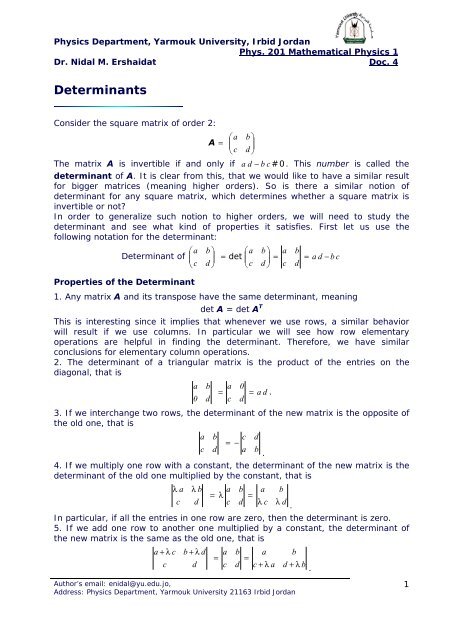
<strong>Determinants</strong><br />
Consider the square matrix of order 2:<br />
⎛a<br />
b ⎞<br />
A = ⎜<br />
⎟<br />
⎝ c d ⎠<br />
The matrix A is invertible if and only if a d − b c # 0 . This number is called the<br />
determinant of A. It is clear from this, that we would like to have a similar result<br />
for bigger matrices (meaning higher orders). So is there a similar notion of<br />
determinant for any square matrix, which determines whether a square matrix is<br />
invertible or not?<br />
In order to generalize such notion to higher orders, we will need to study the<br />
determinant and see what kind of properties it satisfies. First let us use the<br />
following notation for the determinant:<br />
⎛a<br />
b ⎞ ⎛a<br />
b ⎞ a b<br />
Determinant of ⎜<br />
= = a d − b c<br />
c d<br />
⎟ = det ⎜<br />
c d<br />
⎟<br />
⎝ ⎠ ⎝ ⎠ c d<br />
Properties of the Determinant<br />
1. Any matrix A and its transpose have the same determinant, meaning<br />
det A = det A T<br />
This is interesting since it implies that whenever we use rows, a similar behavior<br />
will result if we use columns. In particular we will see how row elementary<br />
operations are helpful in finding the determinant. Therefore, we have similar<br />
conclusions for elementary column operations.<br />
2. The determinant of a triangular matrix is the product of the entries on the<br />
diagonal, that is<br />
a b a 0<br />
= = a d .<br />
0 d c d<br />
3. If we interchange two rows, the determinant of the new matrix is the opposite of<br />
the old one, that is<br />
a b c d<br />
= −<br />
c d a b<br />
.<br />
4. If we multiply one row with a constant, the determinant of the new matrix is the<br />
determinant of the old one multiplied by the constant, that is<br />
λ a λ b a b a b<br />
= λ =<br />
c d c d λ c λ d<br />
.<br />
In particular, if all the entries in one row are zero, then the determinant is zero.<br />
5. If we add one row to another one multiplied by a constant, the determinant of<br />
the new matrix is the same as the old one, that is<br />
a + λ c b + λ d a b a b<br />
= =<br />
c d c d c + λ a d + λ b<br />
.<br />
Author’s email: enidal@yu.edu.jo,<br />
Address: Physics Department, Yarmouk University 21163 Irbid Jordan<br />
1
Note that whenever you want to replace a row by something (through elementary<br />
operations), do not multiply the row itself by a constant. Otherwise, you will easily<br />
make errors (due to Property 4).<br />
6. We have<br />
det (AB) = det(A) det(B)<br />
In particular, if A is invertible (which happens if and only if det (AB) #0), then<br />
© Nidal M. Ershaidat 2007<br />
det<br />
-1<br />
( A ) =<br />
1<br />
det ( A)<br />
If A and B are similar, then det (A) = det(B).<br />
Let us look at an example, to see how these properties work.<br />
Example 1. Evaluate<br />
2<br />
−1<br />
1<br />
.<br />
3<br />
Let us transform this matrix into a triangular one through elementary operations.<br />
We will keep the first row and add to the second one the first multiplied by ½. We<br />
get<br />
2<br />
−1<br />
1 2<br />
=<br />
3 0<br />
1<br />
7 .<br />
2<br />
Using the Property 2, we get<br />
2<br />
0<br />
1<br />
7<br />
2<br />
= 2 ⋅<br />
7<br />
= 7 .<br />
2<br />
Therefore, we have<br />
2<br />
−1<br />
1<br />
= 7<br />
3<br />
which one may check easily.<br />
http://www.sosmath.com/matrix/determ0/determ0.html<br />
Author: M.A. Khamsi<br />
<strong>Determinants</strong> of Matrices of Higher Order<br />
As we said before, the idea is to assume that previous properties satisfied<br />
by the determinant of matrices of order 2, are still valid in general.<br />
So let us see how this works in case of a matrix of order 4.<br />
Example 2. Evaluate<br />
We have<br />
1<br />
5<br />
2<br />
3<br />
2<br />
6<br />
6<br />
1<br />
3<br />
7<br />
4<br />
1<br />
1<br />
5<br />
2<br />
3<br />
4<br />
8<br />
8<br />
2<br />
2<br />
6<br />
6<br />
1<br />
3<br />
7<br />
4<br />
1<br />
1<br />
3<br />
4<br />
8<br />
.<br />
8<br />
2<br />
2<br />
5 6 7 8<br />
= 2<br />
.<br />
1 3 2 4<br />
If we subtract every row multiplied by the appropriate number from the<br />
1<br />
3<br />
1<br />
4<br />
2<br />
2
first row, we get<br />
1 2 3 4 1 2 3 4<br />
5<br />
1<br />
6<br />
3<br />
7<br />
2<br />
8<br />
4<br />
=<br />
0<br />
0<br />
− 4<br />
1<br />
− 8<br />
−1<br />
−12<br />
0<br />
3 1 1 2 0 − 5 − 8 −10<br />
We do not touch the first row and work with the other rows. We<br />
interchange the second with the third to get<br />
1 2 3 4 1 2 3 4<br />
0<br />
0<br />
− 4<br />
1<br />
− 8<br />
−1<br />
−12<br />
0<br />
0<br />
= −<br />
0<br />
1<br />
− 4<br />
−1<br />
− 8<br />
0<br />
.<br />
−12<br />
0 − 5 − 8 −10<br />
0 − 5 − 8 −10<br />
If we subtract every row multiplied by the appropriate number from the<br />
second row, we get<br />
1 2 3 4 1 2 3 4<br />
0<br />
0<br />
1<br />
− 4<br />
−1<br />
− 8<br />
0<br />
−12<br />
=<br />
0<br />
0<br />
1<br />
0<br />
−1<br />
−12<br />
0<br />
−12<br />
.<br />
0 − 5 − 8 −10<br />
0 0 −13<br />
−10<br />
Using previous properties, we have<br />
1 2 3 4 1 2 3 4<br />
0<br />
0<br />
1<br />
0<br />
−1<br />
−12<br />
0<br />
−12<br />
0<br />
= −12<br />
0<br />
1<br />
0<br />
−1<br />
1<br />
0<br />
1<br />
.<br />
0 0 −13<br />
−10<br />
0 0 −13<br />
−10<br />
If we multiply the third row by 13 and add it to the fourth, we get<br />
1 2 3 4 1 2 3 4<br />
0<br />
0<br />
1<br />
0<br />
−1<br />
1<br />
0<br />
1<br />
=<br />
0<br />
0<br />
1<br />
0<br />
−1<br />
1<br />
0<br />
1<br />
0 0 −13<br />
−10<br />
0 0 0 3<br />
which is equal to 3. Putting all the numbers together, we get<br />
1 2 3 4<br />
5<br />
2<br />
6<br />
6<br />
7<br />
4<br />
8<br />
8<br />
= 2 ⋅ ( −1)<br />
⋅ ( −12)<br />
⋅3<br />
= 72.<br />
3 1 1 2<br />
These calculations seem to be rather lengthy. We will see later on that a<br />
general formula for the determinant does exist.<br />
Example 3. Evaluate<br />
© Nidal M. Ershaidat 2007<br />
1<br />
− 1 1 1 .<br />
1<br />
2<br />
2<br />
In this example, we will not give the details of the elementary operations.<br />
We have<br />
1<br />
−<br />
1<br />
1<br />
2<br />
1<br />
2<br />
0<br />
1<br />
3<br />
=<br />
1<br />
0<br />
0<br />
0<br />
3<br />
2<br />
3<br />
0<br />
0<br />
1<br />
3<br />
=<br />
9.<br />
3
Example 4. Evaluate<br />
We have<br />
1<br />
0<br />
2<br />
1<br />
1<br />
1<br />
© Nidal M. Ershaidat 2007<br />
2<br />
1<br />
−1<br />
=<br />
1<br />
0<br />
0<br />
1<br />
0<br />
2<br />
1<br />
1<br />
−1<br />
1<br />
1<br />
1<br />
2<br />
1<br />
− 5<br />
2<br />
1<br />
−1<br />
=<br />
.<br />
1<br />
0<br />
0<br />
1<br />
1<br />
0<br />
2<br />
0<br />
− 5<br />
= − 5.<br />
General Formula for the Determinant<br />
Let A be a square matrix of order n. Write A = (aij), where aij is the entry<br />
on the row number i and the column number j, for i = 1, 2, 3, … n and j =<br />
1, 2, … n. For any i and j, set Aij (called the cofactors) to be the<br />
determinant of the square matrix of order (n-1) obtained from A by<br />
removing the row number i and the column number j multiplied by (-1) i+j .<br />
We have<br />
for any fixed i, and<br />
det<br />
det<br />
( ) ∑ = j<br />
A =<br />
n<br />
a<br />
j = 1<br />
( ) ∑ = i<br />
A =<br />
n<br />
i = 1<br />
for any fixed j. In other words, we have two types of formulas: along a<br />
row (number i) or along a column (number j). Any row or any column will<br />
do. The trick is to use a row or a column which has a lot of zeros.<br />
In particular, we have along the rows<br />
a b c<br />
e f d f d e<br />
d e f = a − b + c<br />
h k g k g h<br />
g h k<br />
or<br />
or<br />
a<br />
d<br />
g<br />
a<br />
d<br />
g<br />
b<br />
e<br />
h<br />
b<br />
e<br />
h<br />
c<br />
f<br />
k<br />
c<br />
f<br />
k<br />
a<br />
i j<br />
i j<br />
A<br />
A<br />
i j<br />
i j<br />
b c a c a b<br />
= − d + e − f ,<br />
h k g k g h<br />
b c a c a b<br />
= g − h + k .<br />
e f d f d e<br />
As an exercise write the formulas along the columns.<br />
Example 5. Evaluate<br />
3<br />
2<br />
4<br />
2<br />
1<br />
0<br />
1<br />
−<br />
3<br />
1<br />
4
We will use the general formula along the third row. We have<br />
3<br />
2<br />
4<br />
2<br />
1<br />
0<br />
1<br />
3<br />
1<br />
2<br />
= 4<br />
1<br />
1<br />
− 3<br />
3<br />
− 0<br />
2<br />
1<br />
− 3<br />
3<br />
+ 1<br />
2<br />
2<br />
= 4 − 6 −1<br />
1<br />
+ 1 3 − 4 = −<br />
− ( ) ( ) 29<br />
Which technique to evaluate a determinant is easier? The answer depends<br />
on the person who is evaluating the determinant. Some like the<br />
elementary row operations and some like the general formula. All that<br />
matters is to get the correct answer.<br />
Note that all of the above properties are still valid in the general case.<br />
Also you should remember that the concept of a determinant only exists<br />
for square matrices.<br />
http://www.sosmath.com/matrix/determ0/determ1.html<br />
Author: M.A. Khamsi<br />
© Nidal M. Ershaidat 2007<br />
5