Determination of spiral orbits with constant tangential velocity - English

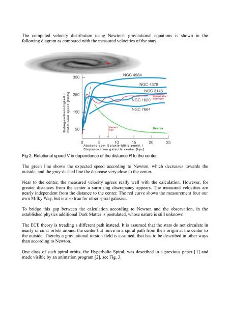
The computed velocity distribution using Newton's gravitational equations is shown in the
following diagram as compared with the measured velocities of the stars.
Fig 2: Rotational speed V in dependence of the distance R to the center.
The green line shows the expected speed according to Newton, which decreases towards the
outside, and the gray-dashed line the decrease very close to the center.
Near to the center, the measured velocity agrees really well with the calculation. However, for
greater distances from the center a surprising discrepancy appears. The measured velocities are
nearly independent from the distance to the center. The red curve shows the measurement four our
own Milky Way, but is also true for other spiral galaxies.
To bridge this gap between the calculation according to Newton and the observation, in the
established physics additional Dark Matter is postulated, whose nature is still unknown.
The ECE theory is treading a different path instead. It is assumed that the stars do not circulate in
nearly circular orbits around the center but move in a spiral path from their origin at the center to
the outside. Thereby a gravitational torsion field is assumed, that has to be described in other ways
than according to Newton.
One class of such spiral orbits, the Hyperbolic Spiral, was described in a previous paper [1] and
made visible by an animation program [2], see Fig. 3.