Visual Based Predictive Control for a Six Degrees of Freedom Robot

Visual Based Predictive Control for a Six Degrees of
Freedom Robot
P.A. Fernandes Ferreira 1 , J.R. Caldas Pinto 2
1 Instituto Politécnico de Setúbal, Escola Superior de Tecnologia,
Campus do Instituto Politécnico de Setúbal, Estefanilha. 2914-508 Setúbal, Portugal
2 Instituto Superior Técnico, Av. Rovisco Pais, 1096 Lisboa, Portugal
e-mail: pferreir@est.ips.pt
Abstract- A visual servoing architecture for a six degrees
of freedom PUMA robot, using predictive control, is
presented. Two different approaches, GPC and MPC,
are used. A comparison between these two ones and the
classical PI controller is performed. The implemented
PUMA robot model simulator used as platform for the
development of the control algorithms is presented. A
control law based on features extracted from camera
images is used. Simulation results show that the
proposed strategies provide an efficient control system
and that visual servoing architectures using predictive
control are faster than those using PI control.
Experimental results are obtained from an architecture
using a XPC Target and Matlab Simulink. Through this
technology is possible to create an operative system
which allows working in real time robot control.
1. INTRODUCTION
The controller has a crucial role in a visual servoing system
performance. Most of the developed works in visual
servoing systems do not take into account the manipulator
dynamics. Nevertheless, considering these parameters could
increase the precision and the velocity of the system.
The term Model Predictive Control (MPC) includes a very
wide range of control techniques which make an explicit use
of a process model to obtain the control signal by
minimizing an objective function [1]. The MPC is often
formulated in a state space formulation conceived for
multivariable constrained control while Generalized
Predictive Control (GPC), which was first introduced in
1987 [2], is primarily suited for single variable, being the
model presented in a polynomial transfer function form.
Predictive control systems have been applied to different
fields such as industry, medicine and chemical process
control. Particularly, Model Predictive control has been
adopted in industry as an efficient way of dealing with
multivariable constrained control problems [3].
A developed work in the field of visual servoing systems for
small displacements used a predictive controller [4]. In this
work, it is given continuity to some developed works in
visual servoing research [5], [6]. In order to carry out this
1-4244-0681-1/06/$20.00 '2006 IEEE
846
work a toolbox that allows incorporating vision in the
PUMA robot control architecture was created. Its great
versatility, allowing the easy interconnection of different
types of controllers, becomes this type of tool very
advantageous. In this paper the results of a set of
experiences in the area of the modelling, identification and
control of a visual servoing system for a PUMA 560 robot
are presented.
This paper is organised as follows: the implemented six
degrees of freedom Puma robot model simulation and its
validation is presented in section 2. A brief overview of a
2D visual servoing technique is introduced in Section 3. The
principles of Predictive Control (GPC and MPC) and the
identification of the PUMA ARMAX model are presented
in Section 4. The experimental settings and the results for a
PI, GPC and MPC controllers are given in section 5. Section
6 concludes the paper and section 7 suggests the continuity
of this work.
2. PUMA 560 MODEL
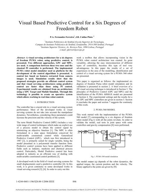
This work started with the implementation of the PUMA
560 model [7] corresponding to a six degrees of freedom
robot model (Fig.1) with all the joints revolute. In order to
validate the model, real tests in joint space with some
controllers and gravity compensation [8] were performed.
1
torque
torque MATLAB
MATLAB
2
Function
Function
Dqout
Saturation
q''
DAC
q' q
Sum6
KrG
MATLAB
1/s
1/s
1
Function
qout
Robot
MATLAB
Function
KG
Out1 In1
Gravitic compensation
Fig. 1. PUMA 560 model simulation
The model output (q) depends of the robot dynamics, the
applied torque, the current position and the velocity. The
binary applied to the joints are given by [9]:
Authorized licensed use limited to: Pontificia Universidad Javeriana. Downloaded on March 23,2010 at 08:17:40 EDT from IEEE Xplore. Restrictions apply.

T= M( qq ) + Cqqq ( , ) + Fq + Gq ( )
(1)
where M is the Inertia matrix, q is the vector joints
velocities, q
is the vector joints acceleration. The matrices
C, F and G represent the Coriolis and centripetal effects, the
viscous and Coulomb Forces, and the gravity effects
respectively.
2.1 Puma model validation
The robot model was tested with a PI controller using the
parameters of the real system. Fig. 2 shows the torque
values for a 20º amplitude trajectory during 9 s. It was used
an algorithm that allows to obtain a planning periodic
trajectory (Fig.2). The error obtained from the comparison
between the real and simulate robot trajectory is shown in
Fig. 3.
Fig. 2. Real and simulation trajectory result of joint 3.
Fig. 3. Error result between real and simulate to joint 3.
3. VISUAL SERVOING ARCHITECTURES
3.1 Basic definitions
A few basic definitions for 2D visual servoing architecture
are here introduced (see Fig. 4.):
pe - Actual pose of the camera (with respect to a fixed
reference frame R0)
p - Required displacement of the camera referential from the
actual position to the desire position, related to the observed
object frame.
p* - Pose of the camera (with respect to a fixed reference
frame R0) in a desired position.
847
Mcr – Homogeneous transformation between the camera
frame in the current position, Rc, and camera frame in the
desired position Rr.
Fig. 4. Reference frames definition.
Let T6 be the transformation which converts a
homogeneous matrix into 6 operational coordinates:
where
p (q)=T6 (Mcr(q)) (2)
Mcr=
⎡r
⎢
⎢
r
⎢r
⎢
⎣ 0
11
21
31
r
r
r
12
22
32
0
r
r
r
13
23
33
0
Tx
⎤
T
⎥
y ⎥
Tz
⎥
⎥
1 ⎦
p(q)= [ ] T
x
y
z
x
y
z
(3)
T T T θ θ θ (4)
Then the homogeneous matrix can be transformed into a
vector that describes the displacement as function of
rotation and translation.
where
R b
p(q) = T6(M )=
⎡
T x
⎤
⎢
⎥
⎢
T y
⎥
⎢
T z
⎥
⎢
⎥
⎢ arcsin( r13
) ⎥
⎢
− r12
r11
⎥
⎢arctan
2(
, )
cos θ cos
⎥
⎢
r θ r ⎥
⎢
− r23
r33
arctan 2(
, ) ⎥
⎢
⎣ cos θ cos r ⎥
r θ ⎦
θ r = arcsin( r13
)
(6)
From the definition of robot Jacobian [9] the relationship
between the joint velocities and the end-effector linear and
angular velocities is given by the expression:
where Jc is the robot Jacobian.
3.2 2D Visual Servoing
x
y
x
p e
y
x
M cr= p
(5)
pq ( ) = J( qq ) (7)
The modelled system describes the PUMA 560 dynamics
with an eye in hand configuration controlling its 6 degrees
Authorized licensed use limited to: Pontificia Universidad Javeriana. Downloaded on March 23,2010 at 08:17:40 EDT from IEEE Xplore. Restrictions apply.
R c
R 0
z
x
Z
c
y
*
p
R r
z
y

of freedom. The camera is placed in such a way that objects
in workspace are in its field of vision. An error image is
measured and used to evaluate the displacement related to
the end effector. Thus the robot pose is estimated through
the visual information. Within this framework image feature
measures are converted in 6 operational coordinates.
Fig. 5 2D Visual Servoing.
The used control architecture represented in Fig. 5 is a 2D
type [10]. The reference is obtained from image features.
This approach uses the robot pose error p=(p*-pe) obtained
from the difference between the reference image features s*
and the obtained current image features s. The image
Jacobian, that relates the kinematics torsor of the camera
frame and the variation of image primitives, plays an
important role.
The extracted visual measure is expressed under the form of
a pose p, which contains six operational coordinates. This
pose is obtained from the relation between the frame Rr in
the desired position and the camera frame in current position
Rc. The control goal consists of bringing the measure p to
the desired measure pr. When p is very close to pr,
Mcr= * M cr , and
Mcr=I (8)
2n
Let s ∈ be the vector of current coordinates of n points
of the image:
s [ x y x y ... x y ]
= (9)
p1
p1
p2
p2
The image Jacobian Jv(s)∈R 2nx6 is a matrix that relates the
velocity s of the image points and the kinematics torsor r
of the camera frame.
where
s *
s
Comand
law
Image primitives
measure
Robot
comand
and the image Jacobian is given by:
Image
processing
pn
pn
s= Jv() s r
(10)
T
r = [ v vyvzωxωyωz] x
R (11)
c
pe
R 0
Target
848
⎡ x x y f + x ⎤
2
f
p1 p1 p1 2 p1
⎢ − 0
−
y p1
⎥
⎢ z1 z1 f f ⎥
⎢ 2 2 1
f f + y p xp1y ⎥
p1
⎢ 0 − yp1 − −xp1⎥
⎢ Z1f f ⎥
Jv
( ℑ ) =
⎢ ⎥
⎢ ⎥
2
⎢ f xpn xpnypn f2+ x ⎥
pn
⎢− 0
−
y pn ⎥
⎢ Zn zn f f ⎥
⎢ 2 2
f ypn f + y pn xpny ⎥
pn
⎢ 0 − − −x⎥
pn
⎢⎣ zn zn f f ⎥⎦
(12)
The image Jacobian is a function of the image features,
focal distance f and of the camera frame z-coordinates of the
target points. The relation between the kinematics torsor r
and p is given by
r = J p
(13)
where Jp is the Jacobian between the referential in initial
and final position and relates the velocity in these two
frames:
p→0
p
lim J p =− I
(14)
Assuming Pr ≈ 0, in case of displacement, and that servoing
is fast enough the following approach is valid:
P ≈ −r
(15)
Let J v + be the pseudo inverse image Jacobian Jv ( s ) , then
From equation (15):
0
J
v
T −1
T ( J J ) J
+ =
(16)
v
v
+
v
v
r= J s
(17)
p ≈−J
s
(18)
Let s0 be the vector of primitives corresponding to the
reference image. When s = s0
, Rc = Rr
and
p = p = 0 . From equation (18) one can deduce:
0
+
v
( ) 2
+
p− p = −J s− s* + O( s ) (19)
v
2
+
where Os ( ) is a second order error component, and J v is
the pseudo-inverse image Jacobian s is the primitive of the
target for the actual configuration of the robot and s0 is the
primitive of the target for the desired robot configuration.
Then
+
p≈−J s− s
(20)
v
( )
From equation (20) is possible to convert image primitive
measures into six operational coordinates P.
Authorized licensed use limited to: Pontificia Universidad Javeriana. Downloaded on March 23,2010 at 08:17:40 EDT from IEEE Xplore. Restrictions apply.
0

4. PREDICTIVE CONTROL
4.1 Generalized Predictive Control
The basic idea of GPC is to calculate a sequence of future
control signals in such a way that it minimizes a cost
function defined over a prediction horizon [1], [2]. The
index to be optimized is the expectation of a quadratic
function measuring the distance between the predicted
system output and some predicted reference sequence over
the horizon plus a quadratic function measuring the control
effort.
H p Hc
2
Jk ( ) = ∑ yˆ − r + λ2
∆u
k+ j k+ j ∑ k+ j−1
j= N j=
1
where:
N1- minimum costing horizons
Hp – Prediction horizon
Hc≤Hp≥1 Control horizon
1
∆uK - Control action increment, ∆uk=uk-uk-1
λk - control energy weight
y ˆ
k + j - Prediction of the system output
- reference predictive trajectory
r k + j
The system model can be presented in the ARMAX form [1]
−1
−1
A( z ) y(
t)
= B(
z ) u(
t −Te
−1
C(
z ) ξ ( t)
) +
−1
1−
z
(22)
1
Where Az ( )
−
1
, Bz ( )
−
1
and Cz ( )
−
are the matrix
parameters of transfer function H ( z ) . To compute the
output predictions is necessary to know the system model
that must be controlled (Fig. 7). The parameters used by the
GPC are obtained from the configuration shown in Fig. 6.
∆ p p *
GPC
H(z)
J -1
∗
q
ZOH
Vision (Z -1 )
F(z)
Fig. 6. Manipulator system block diagram controlled by vision.
The transfer, H ( z ) , function is given by:
q
Jc ∫
Robot
velocity
control
p
(21)
849
pz ( ) − 1 T 11
( ) ( ) a z+
H z = = JcF z Jc
p *( z) 2 z−1z (23)
The parameters of this function are used in the predictive
controller implementation.
4.2 System Identification
The robot model is obtained by identifying each of the joints
dynamics to obtain a six order linear model:
−5 −4 −3 −2 −1
bz 5 + bz 4 + bz 3 + bz 2 + bz 1 + b0
Fi( z)
=
−6 −5 −4 −3 −2 −1
z + a5z + a4z + a3z + a2z + a1z + a0
(24)
In the identification procedure a PRBS is used as input
signal. A prediction error method (PEM) is used to identify
1
the robot dynamics. The noise model Cz ( )
−
of order 1 was
selected. In this approach the identification of H ( z ) (Fig. 6)
is performed around a reference condition. Since the robot is
controlled in velocity and the dynamics depend mainly on
the first joints, assuming small displacements is possible to
linearize the system around the position q. It was also
necessary to consider a diagonal inertia matrix. Under these
conditions, the Jacobian matrix is constant as well as H(z).
This procedure is valid at low velocities. This means that the
cross coupled terms are neglected.
4.3 Model Predictive Controller
In this approach the model is formulated in a space state
form:
⎧x(
t + 1)
= Ax(
t)
+ Bu(
t),
x(
0)
= x0
⎨
⎩ y(
t)
= Cx(
t)
(25)
where x(t) is the state, u(t) is the control input and y(t) is the
output.
p *
p
J B t
∫ Ct J -1
A t
Fig. 7 State space manipulator scheme.
The state space manipulator dynamics controlled in velocity
is represented in Fig. 7. The parameters values of At, Bt and
Ct are obtained from the identification algorithm PEM. The
matrices in equation (25) are computed through the image
Jacobian matrix by the following definitions:
B = BJ C= CJ A= A (26)
−1
t t t
The predictive control algorithm is (Clarke et al., 1987):
Authorized licensed use limited to: Pontificia Universidad Javeriana. Downloaded on March 23,2010 at 08:17:40 EDT from IEEE Xplore. Restrictions apply.

1. At time t predict the output from the system,
y ˆ( t + k / t)
, where k=N1,N1+1,…,N2.These outputs
will depend on the future control signals,
u ˆ( t + j / t)
, j=0,1,…,N3 and on the measured state
vectors at time t.
2. Choose a criterion based on these variables and
optimise with respect to u ˆ( t + j / t),
j = 0,
1,...,
N 3 .
3. Apply u ( t)
= uˆ
( t / t)
.
4. At time t+1 go to 1 and repeat.
5.1 System configuration
5. SIMULATION PROCEDURE
The implemented Visual Servoing package allows the
simulation of different kind of cameras. In this particular
case, it was chosen a Costar camera placed in the endeffector
and positioned according with oz axis. Its target of
eight coplanar points was created which will serve as
control reference. The accuracy of the camera position
control in the world coordinate system was increased by the
use of redundant features [11]. The centre of the target
corresponds to the point with coordinates (0,0) and the
remaining points are placed symmetrically in relation to this
point. The target pose is referenced to the robot base frame.
In the case of servoing a trajectory, the target is remained
fixed and the desired point is variable. As the primitive of
the target points is obtained it is possible to estimate the
operational coordinates of the camera position point.
Visual Servoing with a PI controller. In 2D Visual Servoing
the image characteristics are used to control the robot.
Images acquired by the camera are function of the end
effector’s position, since the camera is fixed on the end
effector of the robot. They are compared with the
corresponding desired images. In the present case the image
characteristics are the centroids of the target points. Fig. 8
represents the model simulation of the implemented 2D
visual servoing architecture. In this case CT is a PI
controller.
dp,pd
pd
dp
CT
P-P*
S0
Jr
J v
ZOH
+
− S
Fig. 8 2D visual servoing architecture simulation.
Predictive Visual Servoing implementation. In this approach
our goal is also to control the relative pose of the Robot in
respect to the target. In a similar way the model corresponds
to Fig. 8 but substituting the controller – in a first case is
used a GPC and in another is used a MPC controller. In both
experiments all the conditions and characteristics of the
robot are the same. The goal is to control the end effector
from the image error between a current image and desire
image.
q iin
q out
Puma 560 + control
850
5.2 Visual servoing control results
Visual Servoing using a PI Controller. To eliminate the
position error was chosen a PI controller. The point
coordinates in operational coordinates are:
pi = [0.35 –0.15 0.40 π 0 π] T
pd = [0.45 –0.10 0.40 π 0 π] T
The points pi and pd correspond to the Robot position from
which the images used to control the robot are obtained. In
Fig. 7 it can be observed the translation and rotation of the
end-effector around ox, oy and oz axis.
Fig. 9 Visual servoing using PI control.
Predictive GPC and MPC Visual servoing control. In both
experiments a 2D visual servoing architecture were used.
From figures 9, 10 and 11 it can be seen that the GPC has a
more linear trajectory and is faster. The rise time is around
0.6s for the PI while for the GPC and MPC are 0.1s and
0.2s, respectively. The settling time is 1s for the PI, 0.3s for
the GPC and 0.9s for the MPC. The results are less accurate
in turn of z and for rotation of the end-effector.
Fig. 10 Results of a 2D Visual servoing architecture using a GPC
controller.
Fig 11 Results of a 2D Visual servoing architecture using a MPC
controller.
Authorized licensed use limited to: Pontificia Universidad Javeriana. Downloaded on March 23,2010 at 08:17:40 EDT from IEEE Xplore. Restrictions apply.

Table 1 presents the computed errors for each algorithm
which reveals the best performance for the GPC.
TABLE1
r.m.s. values for the control algorithm
SSR Tx Ty Tz θx θy θz error
PI 2.50 2.40 1.20 2.20 0.30 0.47 1.51
GPC 2.14 0,81 0.22 1.84 0.22 0.02 0.87
MPC 1.36 0.67 3.01 0.76 6.3 6.21 3.04
6. EXPERIMENTAL PROCEDURE
The experimental implementation of the proposed vision
control algorithms was performed through the whole
simulation system previously developed used as platform. In
spite of the presented simulation works had been developed
in an “eye in hand” configuration, the experimental works
were performed according to an “eye to hand” one. This
fact is related with the necessity of protecting the camera
which was placed outside the robot allowing from this way a
higher security system in the initial phase.
The homogeneous transformation matrix which relates the
camera frame with the robot frame, w
T c , for the used
configuration is given by:
w Tc
⎡−1000.4521⎤ ⎢
0 0 −1
0.45
⎥
= ⎢ ⎥
⎢ 0 −1
0 0.91 ⎥
⎢ ⎥
⎣ 0 0 0 1 ⎦
(27)
The application consisted in the robot control using in a first
one a PI controller and in a second one a generalized
predictive controller, GPC.
6.1 Implemented system configuration
In the experimental developed work the potentiality given
by the XPC Target and Matlab Simulink was used. Through
this technology is possible to create an operative system
which allows working in real time robot control. There were
used two computers (Fig. 12), a Host-PC used for the visual
information acquisition and processing and a target PC
which receives the processing results from the Host-PC and
performs the robot control.
The image acquisition system processes them at a rate
between 12 and 20 images per second and sends the
processed data to the robot control system (Target PC)
through RS232. This external loop control frequency is
related with the algorithm weight, the numerical capacity of
the computers and with the specific weight of the simulink
program. Theoretically the used Vector camera could reach
the rate of 300 images per second.
In order to generate the robot control environment it was
necessary to replace the original PUMA controller by an
open control architecture. This procedure allows the
851
adaptation of the system to different kinds of controllers. In
the present case the internal controller was substituted by a
velocity controller with gravitic compensation.
host
Image information
Visual control algorithm
target
Fig 12 Experimental Scheme.
The target target view by the camera is shown in figure 13.
A planar target with 8 LED’s, placed at the vertices of two
squares of 40 mm of side and spacing to each other of 150
mm, is used. In figure 13 is possible to observe the target
viewed by the camera.
The choice of the number of points was conditioned by the
estimated sensibility from the obtained results in the
theoretical study obtained through simulation and by the
limitations of the image processing system. In spite of
having redundant information this number of points lead to
better results as it was verified in the simulation study.
Fig. 13 Target view by the camera.
The experimental works obey to the configurations shown
in figure 14.
Fig. 14 Installation of the experimental visual servoing system.
The image that would be used as reference was previously
captured. From this one the image primitives were obtained
and corresponded to the centroids of 8 lighting circles
Authorized licensed use limited to: Pontificia Universidad Javeriana. Downloaded on March 23,2010 at 08:17:40 EDT from IEEE Xplore. Restrictions apply.
t

shown in figure 5.8. The end effectors or more precisely the
target was displaced 30º away from that position around
joint 3. The robot tries to reach the desired position through
the control scheme shown in figure 8. In spite of the
performed displacement correspond to the simple situation
of moving around a joint, the followed trajectory is realized
by the use of the other joints. The goal of the task performed
by the robot will be to place the target in a position which
corresponds to the desired image. Therefore the robot
manipulator follows a trajectory in order to minimize the
s − s .
error between the current and reference images, ( )
In the experiments carried out two different controllers were
used: proportional and predictive. As in the simulation case
the robot is controlled in velocity through the internal loop
which includes gravitic compensation. This one operates at
frequency of 1 KHz and the external vision controller
operates at a frequency of 12 Hz.
6.2 Experimental results of the vision control system using a
proportional controller
In the experimental work it was concluded that very
reasonable results were obtained through the use of a
proportional controller and that the integrative or derivative
factor had no influence on the system performance
From figure15 is possible to evaluate the images error in a
2D visual servoing architecture using a proportional
controller. The good system convergence is notable and one
can observe that the error is near zero approximately after
20 seconds for all the image primitives.
Image error (pixels)
Time (s)
Fig. 15 Image error for the 2D architecture using a PI controller.
6.3 Experimental results of the vision control
system using a predictive controller
From the developed work presented the predictive control
algorithm presented was implemented. A prediction horizon
of H p = 6 was used.
The implementation of the predictive control algorithm was
preceded by the identification of the ARIMAX model for
each of the controlled joints. In the identification procedure
a PRBS (pseudo random binary signal) with a frequency of
100 Hz was injected in each joint. The Identification
algorithm based on the prediction error [12] was used.
d
852
From figure 16 is possible to evaluate the image results
through the use of a generalized predictive control
algorithm. The good convergence is notable and one can
conclude that this system is faster when compared with the
use of a proportional controller. The error is near zero
approximately after 15 seconds for all the image primitives.
Fig. 16 Image error for the 2D architecture using a GPC controller.
From figure 17 the joint velocity evolution for the case of
using a GPC and a PI controller can be observed. The joint
velocities are lower than in the proportional controller case
as well of the oscillations.
Joint velocity (rad/s)
Image error (pixels)
Time (s)
(a)
Time (s)
Fig. 17 Joint velocity using a 2D architecture with a GPC (a) and a PI (b)
controller.
Joint velocity (rad/s)
7. CONCLUSIONS
Time (s)
(b)
A vision control system applied to a six degrees of freedom
robot was studied. A PUMA 560 model was carried out and
tested with a PI controller using the parameters of the real
system. A prediction error method was used to identify the
robot dynamics and to implement a predictive control
algorithm (MPC and GPC). The three different algorithms
always converge to the desired position. In general, we can
conclude that in visual servoing is obvious the good
performance of both predictive controllers. The obtained
results also show that the 2D algorithm associated with the
studied controllers allows to control larger displacements
than those referred in [4].
From the analysis of r.m.s error presented in Table 1 we can
conclude the better performance of the GPC. In spite of the
better MPC results for the translation in the xy plane when
compared to the GPC, the global error is worse. In the visual
servoing trajectory is obvious the good performance of this
approach. The identification procedure has a great influence
on the results.
Authorized licensed use limited to: Pontificia Universidad Javeriana. Downloaded on March 23,2010 at 08:17:40 EDT from IEEE Xplore. Restrictions apply.

The evaluation of the graphical trajectories and the
computed errors allow finally concluding that the GPC
vision control algorithm leads to the best performance.
Finally the obtained experimental results for the “eye to
hand” case are in agreement with those expected from the
theoretical algorithm development and the simulation
results. The developed experimental system allows using
with great versatility the simulation algorithms.
8. FUTURE WORKS
In future works, another kind of controllers such as
intelligent, neural and fuzzy will be used. Other algorithms
to estimate the joints coordinates should be tested. These
algorithms will be applied to the real robot in visual
servoing path planning. Furthermore others target and other
visual features should be tested.
ACKNOWLEDGEMENTS
This work is partially supported by the “Programa de
Financiamento Plurianual de Unidades de I&D (POCTI), do
Quadro Comunitário de Apoio III” by program FEDER and
by the FCT project POCTI/EME/39946/2001.
REFERENCES
[1] Camacho, E. F. and C. Bordons (1999). Model
Predictive Control. Springer Berlin
[2] Clarke, D.W., C.Mohtafi, and P.S.Tuffs. Generalized
Predictive Control-Part I (1987). The Basic
Algorithm, Automatica, Vol.23, Nº2, pp.137-148.
[3] Lee, J.H,. and B. Cooley (1997). Recent advances in
model predictive control.In:Chemical Process Control,
Vol.93, no. 316. pp201-216b. AIChe Syposium Series
– American Institute of Chemical Engineers.
[4] Gangloff, J. (1999). Asservissements visuel rapides D’
un Robot manipulateur à six degrés de liberté. Thèse
de Doutorat de L’ Université Louis Pasteur.
[5] Corke, P. (1994). A Search for Consensus Among Model
Parameters Reported for the Puma 560 In Proc. IEEE
Int. Conf.. Robotics and Automation, pages 1608-
1613, San Diego.
[6] Malis,E., F. Chaumette and S. Boudet 1999. 21/2D
visual Servoing. IEEE Transactions on Robotics and
Automation 15 (2), 238-250.
[7] Chaumette, F. (1990). La relation vision-commande:
théorie et application à des tâches robotiques. Thése de
doctorat, Université de Rennes.
[8] Craig, J. (1988). Adaptive Control of Mechanical
Manipulators, Addison-Wesley.
[9] Sciliano, B. and L Sciavicco 2000. Modelling and
Control of Robot Manipulators, 2 nd edition,
Springer-Verlag.
[10] Ferreira, P. e Caldas, P. (2003). 3D and 2D Visual
servoing Architectures for a PUMA 560 Robot. In
853
Proceedings of the 7 th IFAC Symposium on Robot
Control, September 1-3, , pp 193-198.
[11] Hashimoto, K. and T. Noritsugu (1998). Performance
and Sensitivity in Visual Servoing. IEEE Int. Conf. on
Robotics and Automation, Leuven, Belgium, pp.2321-
2326.
[12] Ljung, L. (1987). System Identification Theory For
The User, Prentice Hall, Englewood Cliffs, New York.
Authorized licensed use limited to: Pontificia Universidad Javeriana. Downloaded on March 23,2010 at 08:17:40 EDT from IEEE Xplore. Restrictions apply.