Answers - Millersville University

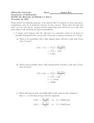
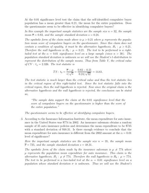
At the 0.01 significance level test the claim that the self-identified compulsive buyer
population has a mean greater than 0.21, the mean for the entire population. Does
the questionnaire seem to be effective in identifying compulsive buyers?
In this example the important sample statistics are the sample size n = 32, the sample
mean x = 0.83, and the sample standard deviation s = 0.24.
The symbolic form of the claim made above is µ > 0.21 where µ represents the population
mean score of compulsive buyers on the questionnaire. Since this claim does not
contain a condition of equality, it must be the alternative hypothesis, H1 : µ > 0.21.
Therefore the null hypothesis is H0 : µ = 0.21. The test to be performed is a righttailed
test at the α = 0.01 significance level on a large sample (since n > 30). The
population standard deviation is unknown so we will use the Student’s t-distribution to
represent the distribution of the sample means. Thus from Table V, the critical value
of CV : tα = 2.326. The test statistic is
TS : t0 =
x − µ
s/ √ n
= 0.83 − 0.21
0.24/ √ 32
= 14.61.
The test statistic is much larger than the critical value and thus the test statistic lies
in the critical region of this right-tailed test. Since the test statistic falls into the
critical region, then the null hypothesis is rejected. Now since the original claim is the
alternative hypothesis and the null hypothesis is rejected, the conclusion can be stated
as,
“The sample data support the claim at the 0.01 significance level that the
score of compulsive buyers on the questionnaire is higher than the score of
the entire population.”
The questionnaire seems to be effective at identifying compulsive buyers.
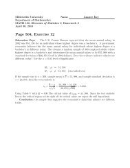
3. According to the Insurance Information Institute, the mean expenditure for auto insurance
in the United States was $774 in 2002. An insurance salesman obtains a random
sample of 35 auto insurance policies and determines the mean expenditure to be $735
with a standard deviation of $48.31. Is there enough evidence to conclude that the
mean expenditure for auto insurance is different from the 2002 amount at the α = 0.01
level of significance?
Here the important sample statistics are the sample size n = 35, the sample mean
x = 735, and the sample standard deviation s = 48.31.
The symbolic form of the claim made by the insurance salesman is µ = 774 where
µ represents the population mean expenditure for auto insurance. This claim is the
alternative hypothesis, H1 : µ = 774. Therefore the null hypothesis is H0 : µ = 774.
The test to be performed is a two-tailed test at the α = 0.01 significance level on a
population whose standard deviation σ is unknown. Thus we will use the Student’s