Answers - Millersville University
Answers - Millersville University
Answers - Millersville University

Create successful ePaper yourself
Turn your PDF publications into a flip-book with our unique Google optimized e-Paper software.
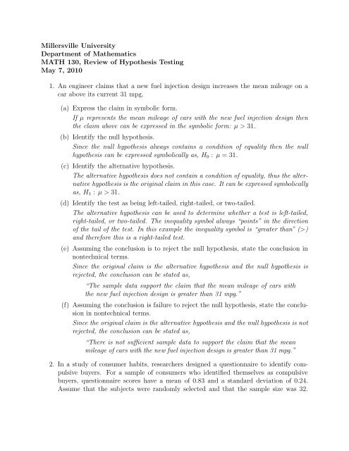
<strong>Millersville</strong> <strong>University</strong><br />
Department of Mathematics<br />
MATH 130, Review of Hypothesis Testing<br />
May 7, 2010<br />
1. An engineer claims that a new fuel injection design increases the mean mileage on a<br />
car above its current 31 mpg.<br />
(a) Express the claim in symbolic form.<br />
If µ represents the mean mileage of cars with the new fuel injection design then<br />
the claim above can be expressed in the symbolic form: µ > 31.<br />
(b) Identify the null hypothesis.<br />
Since the null hypothesis always contains a condition of equality then the null<br />
hypothesis can be expressed symbolically as, H0 : µ = 31.<br />
(c) Identify the alternative hypothesis.<br />
The alternative hypothesis does not contain a condition of equality, thus the alternative<br />
hypothesis is the original claim in this case. It can be expressed symbolically<br />
as, H1 : µ > 31.<br />
(d) Identify the test as being left-tailed, right-tailed, or two-tailed.<br />
The alternative hypothesis can be used to determine whether a test is left-tailed,<br />
right-tailed, or two-tailed. The inequality symbol always “points” in the direction<br />
of the tail of the test. In this example the inequality symbol is “greater than” (>)<br />
and therefore this is a right-tailed test.<br />
(e) Assuming the conclusion is to reject the null hypothesis, state the conclusion in<br />
nontechnical terms.<br />
Since the original claim is the alternative hypothesis and the null hypothesis is<br />
rejected, the conclusion can be stated as,<br />
“The sample data support the claim that the mean mileage of cars with<br />
the new fuel injection design is greater than 31 mpg.”<br />
(f) Assuming the conclusion is failure to reject the null hypothesis, state the conclusion<br />
in nontechnical terms.<br />
Since the original claim is the alternative hypothesis and the null hypothesis is not<br />
rejected, the conclusion can be stated as,<br />
“There is not sufficient sample data to support the claim that the mean<br />
mileage of cars with the new fuel injection design is greater than 31 mpg.”<br />
2. In a study of consumer habits, researchers designed a questionnaire to identify compulsive<br />
buyers. For a sample of consumers who identified themselves as compulsive<br />
buyers, questionnaire scores have a mean of 0.83 and a standard deviation of 0.24.<br />
Assume that the subjects were randomly selected and that the sample size was 32.
At the 0.01 significance level test the claim that the self-identified compulsive buyer<br />
population has a mean greater than 0.21, the mean for the entire population. Does<br />
the questionnaire seem to be effective in identifying compulsive buyers?<br />
In this example the important sample statistics are the sample size n = 32, the sample<br />
mean x = 0.83, and the sample standard deviation s = 0.24.<br />
The symbolic form of the claim made above is µ > 0.21 where µ represents the population<br />
mean score of compulsive buyers on the questionnaire. Since this claim does not<br />
contain a condition of equality, it must be the alternative hypothesis, H1 : µ > 0.21.<br />
Therefore the null hypothesis is H0 : µ = 0.21. The test to be performed is a righttailed<br />
test at the α = 0.01 significance level on a large sample (since n > 30). The<br />
population standard deviation is unknown so we will use the Student’s t-distribution to<br />
represent the distribution of the sample means. Thus from Table V, the critical value<br />
of CV : tα = 2.326. The test statistic is<br />
TS : t0 =<br />
x − µ<br />
s/ √ n<br />
= 0.83 − 0.21<br />
0.24/ √ 32<br />
= 14.61.<br />
The test statistic is much larger than the critical value and thus the test statistic lies<br />
in the critical region of this right-tailed test. Since the test statistic falls into the<br />
critical region, then the null hypothesis is rejected. Now since the original claim is the<br />
alternative hypothesis and the null hypothesis is rejected, the conclusion can be stated<br />
as,<br />
“The sample data support the claim at the 0.01 significance level that the<br />
score of compulsive buyers on the questionnaire is higher than the score of<br />
the entire population.”<br />
The questionnaire seems to be effective at identifying compulsive buyers.<br />
3. According to the Insurance Information Institute, the mean expenditure for auto insurance<br />
in the United States was $774 in 2002. An insurance salesman obtains a random<br />
sample of 35 auto insurance policies and determines the mean expenditure to be $735<br />
with a standard deviation of $48.31. Is there enough evidence to conclude that the<br />
mean expenditure for auto insurance is different from the 2002 amount at the α = 0.01<br />
level of significance?<br />
Here the important sample statistics are the sample size n = 35, the sample mean<br />
x = 735, and the sample standard deviation s = 48.31.<br />
The symbolic form of the claim made by the insurance salesman is µ = 774 where<br />
µ represents the population mean expenditure for auto insurance. This claim is the<br />
alternative hypothesis, H1 : µ = 774. Therefore the null hypothesis is H0 : µ = 774.<br />
The test to be performed is a two-tailed test at the α = 0.01 significance level on a<br />
population whose standard deviation σ is unknown. Thus we will use the Student’s
t-distribution. The number of degrees of freedom is df = n − 1 = 34. Thus from Table<br />
V, the critical value of CV : tα/2 = ±2.728. The test statistic is<br />
TS : t0 =<br />
x − µ<br />
s/ √ n<br />
= 735 − 774<br />
48.31/ √ 35<br />
= −4.776.<br />
Since the test statistic falls into the critical region, the null hypothesis is rejected. Now<br />
since the original claim is the alternative hypothesis and the null hypothesis is rejected,<br />
the conclusion can be stated as,<br />
“The sample data support the claim at the 0.01 significance level that the<br />
mean expenditure for auto insurance is different from $774.”<br />
4. An advertising agency claims that the mean length of television commercials is less<br />
than 30 seconds.<br />
(a) Express the claim in symbolic form.<br />
If µ represents the mean length of commercials, then the claim above can be expressed<br />
in the symbolic form: µ < 30.<br />
(b) Identify the null hypothesis.<br />
Since the null hypothesis always contains a condition of equality then the null<br />
hypothesis is the logical opposite of the claim above. The null hypothesis can be<br />
expressed symbolically as, H0 : µ = 30.<br />
(c) Identify the alternative hypothesis.<br />
The alternative hypothesis does not contain a condition of equality, thus the alternative<br />
hypothesis is the original claim in this case. It can be expressed symbolically<br />
as, H1 : µ < 30.<br />
(d) Identify the test as being left-tailed, right-tailed, or two-tailed.<br />
The alternative hypothesis can be used to determine whether a test is left-tailed,<br />
right-tailed, or two-tailed. The inequality symbol always “points” in the direction<br />
of the tail of the test. In this example the inequality symbol is “less than” (
“There is not sufficient sample data to support the claim that the mean<br />
length of commercials is less than 30 seconds.”<br />
5. A pharmaceutical company makes a pill intended for children susceptible to seizures.<br />
The pill is supposed to contain 20.0 mg of phenobarbital. A random sample of 20 pills<br />
yielded the amounts (in mg) listed below. Do the pills contain the proper amount of<br />
phenobarbital at the α = 0.01 significance level? (Hint: The sample standard deviation<br />
of the weights is s = 3.5.)<br />
27.5 26.0 22.9 23.5 23.0<br />
23.9 26.3 20.9 22.5 21.7<br />
28.4 16.1 19.3 17.2 17.9<br />
21.7 23.0 16.5 24.1 22.3<br />
(a) State the original claim in symbolic form.<br />
If µ represents the mean amount of phenobarbital measured in milligrams in the<br />
pills, then the claim above can be expressed in the symbolic form: µ = 20.0.<br />
(b) In non-technical language describe the type II error for this hypothesis test.<br />
A type II error occurs when a we fail to reject a false null hypothesis. In this<br />
case a type II error occurs when we fail to reject claim that the pills contain an<br />
average of 20.0 milligrams of phenobarbital, when in fact they do not contain that<br />
amount.<br />
(c) Find the critical value of t for this hypothesis test.<br />
Since the sample size is only n = 20, which is considered a small sample, we must<br />
use the Student-t Distribution. The degrees of freedom becomes df = 19. The<br />
original claim is the null hypothesis. The alternative hypothesis is the claim that<br />
µ = 20.0 and thus we are conducting a two-tailed test. The critical value of t is<br />
the value of t for a two-tailed test with α = 0.01 and df = 19. From the Student-t<br />
table this value is tα/2 = ±2.86.<br />
(d) Do the pills contain the proper amount of phenobarbital at the α = 0.01 significance<br />
level?<br />
We must calculate the sample mean before we can find the test statistic.<br />
The test statistic is then<br />
t0 =<br />
x =<br />
x<br />
n<br />
= 444.7<br />
20<br />
≈ 22.24<br />
x − µ<br />
s/ √ 22.24 − 20.0<br />
=<br />
n 3.5/ √ ≈ 2.862.<br />
20<br />
The test statistic is (barely) larger than the critical value. Thus we reject the null<br />
hypothesis. We conclude that the sample data warrant rejection of the claim that<br />
the mean amount of phenobarbital in the pills is 20.0 milligrams.
6. A newspaper survey was the basis for a report that “55% of gun owners favor stricter<br />
gun laws.” Assume that the survey group consisted of 504 randomly selected gun<br />
owners. Test the claim that the majority (more than 50%) of gun owners favor stricter<br />
gun laws. Use a 0.01 significance level.<br />
(a) State the null and alternative hypotheses in symbolic form.<br />
The original claim is that the proportion of gun owners favoring stricter gun laws<br />
is greater than 0.50. The original claim lacks a condition of equality and is thus<br />
the alternative hypothesis. Therefore the null and alternative hypotheses can be<br />
expressed in symbolic form as<br />
H0 : p = 0.50<br />
H1 : p > 0.50<br />
(b) Find the value of the test statistic for this hypothesis test.<br />
Based on the survey data mentioned we see that the sample proportion of gun<br />
owners favoring stricter gun laws is ˆp = 0.55. The value of test statistic is then<br />
z0 =<br />
ˆp − p<br />
p(1−p)<br />
n<br />
= 0.55 − 0.50<br />
(0.50)(1−0.50)<br />
504<br />
≈ 2.24.<br />
(c) Find the critical value for this hypothesis test at the 0.01 significance level.<br />
By examining the alternative hypothesis, we see that we are conducting a righttailed<br />
test with α = 0.01. According to the normal probability table, the critical<br />
value zα = 2.33.<br />
(d) Test the claim that the majority (more than 50%) of gun owners favor stricter<br />
gun laws.<br />
Since the test statistic does not fall in the critical region, we fail to reject the null<br />
hypothesis. Therefore we conclude that the sample data do not support the claim<br />
that the majority of gun owners favor stricter gun laws.<br />
z 2.24<br />
0 zΑ2.33 zΑ2.33
7. A dental X-ray machine bears a label stating that the machine gives radiation dosages<br />
with a mean of less than 5.00 milliroentgens. Sample data consist of 23 randomly<br />
selected observations with a mean of 4.13 milliroentgens and a standard deviation 1.91<br />
milliroentgens. Using a 0.01 level of significance, test the claim stated on the label.<br />
(a) State the label’s claim in symbolic form.<br />
If µ represents the mean X-ray dosage given by the machine, then the original<br />
claim is that µ < 5.00.<br />
(b) Is the original claim the null or alternative hypothesis?<br />
Since the original claim does not contain a condition of equality, it is the alternative<br />
hypothesis, H1 : µ < 5.00.<br />
(c) Find the critical value for this hypothesis test.<br />
Since the sample size is only n = 23, which is considered a small sample, we must<br />
use the Student-t Distribution. The degrees of freedom becomes df = n − 1 = 22.<br />
The alternative hypothesis is the claim that µ < 5.00 and thus we are conducting<br />
a left-tailed test. The critical value of t is the value of t for a one-tailed test with<br />
α = 0.01 and df = 22. From the Student-t table this value is tα = −2.51.<br />
(d) Using a 0.01 level of significance, test the claim stated on the label.<br />
The test statistic is<br />
t0 =<br />
x − µ<br />
s/ √ n<br />
= 4.13 − 5.00<br />
1.9/ √ 23<br />
≈ −2.20.<br />
The test statistic does not fall into the critical region and thus we fail to reject the<br />
null hypothesis. We conclude that the sample data do not support the claim that<br />
the mean radiation dosage given by the machine is less than 5.00 milliroentgens.<br />
t 2.20<br />
tΑ2.51 tΑ2.51<br />
8. The quality control manager of a company which produces telephone-answering machines<br />
considers production to be “out of control” when the overall rate of defects<br />
0
exceeds 4%. Testing of a random sample of 150 machines reveals that 9 are defective,<br />
so the sample percentage of defective answering machines is 6%. The manager claims<br />
that this is only a chance occurrence, so that production is not really out of control.<br />
Use a 0.05 significance level to test the manager’s claim.<br />
In this example the important sample statistics are the sample size n = 150 and the<br />
sample proportion ˆp = x/n = 9/150 = 0.06.<br />
The symbolic form of the claim made above is p ≤ 0.04 where p represents the fraction<br />
of defective answering machines. Since the manager is claiming that production is not<br />
out of control then he is claiming that the defect rate is not exceeding (and therefore<br />
less than or equal to) 4%. Since this claim contains a condition of equality, it is the<br />
null hypothesis, H0 : p = 0.04. Therefore the alternative hypothesis is H1 : p > 0.04.<br />
The test to be performed is a right-tailed test at the α = 0.05 significance level on a<br />
large sample (since n > 30). Thus from the normal probability distribution, the critical<br />
value of zα = 1.645. The test statistic is<br />
z0 =<br />
ˆp − p<br />
<br />
p(1 − p)/n =<br />
0.06 − 0.04<br />
<br />
0.04(1 − 0.04)/150<br />
z 1.25<br />
0 zΑ1.645 zΑ1.645<br />
= 1.25.<br />
Since the test statistic does not fall into the critical region, then the null hypothesis is<br />
not rejected. Now since the original claim is the null hypothesis and the null hypothesis<br />
is not rejected, the conclusion can be stated as,<br />
“The sample data do not warrant rejection of the claim at the 0.05 significance<br />
level that the defect rate of the answering machines is less than or<br />
equal to 4%.”<br />
Production does not seem to be out of control at the answering machine factory.<br />
9. A newspaper ran a report about a <strong>University</strong> of Southern California poll of 1245<br />
students from the western United States. It was reported that 8% of those surveyed
elieve that Jim Morrison (of The Doors) is still alive. The newspaper article began<br />
with the claim that “almost 1 out of 10” students thinks that Jim Morrison is alive.<br />
At the α = 0.025 significance level, test the claim that the true percentage is less than<br />
10%.<br />
(a) Identify the type I error for this test.<br />
Type I error is made when we reject a true null hypothesis. The original claim<br />
is that the proportion of students from the western US who believe Jim Morrison<br />
is still alive is less than 10%. Expressed in symbolic form this is p < 0.10. Since<br />
that statement does not contain a condition of equality, the original claim is the<br />
alternative hypothesis. The null hypothesis is H0 : p = 0.10. Thus the Type I<br />
error in this situation would be the mistake of rejecting the claim that at least<br />
10% of students in the western US believe that Jim Morrison is still alive, when<br />
in fact it is true that at least 10% of students in the western US believe that Jim<br />
Morrison is still alive.<br />
(b) Is the original claim the null or alternative hypothesis?<br />
Based on the discussion in the answer to the previous point, the original claim is<br />
the alternative hypothesis.<br />
(c) Find the critical value for this hypothesis test.<br />
Examining the alternative hypothesis H1 : p < 0.10 we determine that we are<br />
conducting a left-tailed test. The significance level is α = 0.025. From the normal<br />
probability table then the critical value of z is zα = −1.96.<br />
(d) At the 0.025 significance level, test the claim that the true percentage is less than<br />
10%.<br />
Based on the survey data mentioned we see that the sample proportion of gun<br />
owners favoring stricter gun laws is ˆp = 0.08. The value of test statistic is then<br />
z0 =<br />
ˆp − p<br />
p(1−p)<br />
n<br />
= 0.08 − 0.10<br />
(0.10)(1−0.10)<br />
1245<br />
≈ −2.35.<br />
Since the test statistic falls in the critical region we reject the null hypothesis.<br />
Therefore we conclude that the sample data support the claim that the percentage<br />
of students in the western United States who believe that Jim Morrison is alive is<br />
less than 10%.
z 2.35<br />
zΑ1.96 zΑ1.96<br />
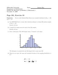
10. When the contents of 1200 boxes of cereal were weighed, 432 were found to be underweight.<br />
Construct the 96% confidence interval estimate for the proportion of cereal<br />
boxes which are underweight.<br />
A cereal box is either underweight or not, so this is yet another example of a binomial<br />
experiment. The sample size is large (n = 1200 > 30). The random variable describing<br />
the number of underweight boxes in the sample is x = 432. The sample proportion of<br />
underweight cereal boxes is<br />
ˆp = x 432<br />
= = 0.360<br />
n 1200<br />
The sample of proportion of non-underweight boxes is 1 − ˆp = 1 − 0.360 = 0.640.<br />
We will use the normal distribution to approximate the binomial distribution. At the<br />
96% confidence level the value of α = 0.04 and thus α/2 = 0.02. The critical value<br />
corresponding to probability 0.5 − 0.02 = 0.48 is zα/2 = 2.054 according to Table V.<br />
Thus the margin of error in this estimate of the population proportion is<br />
E = zα/2<br />
<br />
ˆp(1 − ˆp)<br />
n<br />
= 2.054<br />
0<br />
<br />
(0.360)(0.640)<br />
1200<br />
≈ 0.028<br />
Note that we are rounding the margin of error to three decimal places just like the<br />
sample proportions. Therefore the 96% confidence interval estimate of the sample proportion<br />
of underweight cereal boxes is<br />
(ˆp − E, ˆp + E) = (0.360 − 0.028, 0.360 + 0.028) = (0.332, 0.388).<br />
11. An earlier survey showed that 57% of adults had seen the movie Titanic.<br />
(a) How many people must be surveyed to produce a sample proportion in error by<br />
no more than 3% at the 95% confidence level?<br />
We are being asked to estimate a sample size when we know a previous estimate<br />
of the proportion of adults who have seen the movie is 57% or in other words
ˆp = 0.570. Therefore 1 − ˆp = 1 − 0.570 = 0.430. The margin of error in our<br />
estimate should be 3% or E = 0.03. At the 95% confidence level the value of<br />
α = 0.05 and thus α/2 = 0.025. The critical value corresponding to probability<br />
0.5 − 0.025 = 0.475 is zα/2 = 1.960 according to Table V. Thus the sample size<br />
needed for this estimate is<br />
n =<br />
<br />
zα/2<br />
2<br />
ˆp(1 − ˆp) =<br />
E<br />
2 1.96<br />
(0.570)(0.430) = 1046.2 ≈ 1047<br />
0.03<br />
Notice that we must always round sample sizes up to the next whole number.<br />
(b) How many people must be surveyed if no prior estimate of the sample proportion<br />
is available?<br />
We are being asked to estimate a sample size when no previous estimate of the<br />
proportion of adults who have seen the movie is available, in other words we do<br />
not know ˆp. The margin of error in our estimate should be 3% or E = 0.03. At<br />
the 95% confidence level the value of α = 0.05 and thus α/2 = 0.025. The critical<br />
value corresponding to probability 0.5 −0.025 = 0.475 is zα/2 = 1.960 according to<br />
Table V. Thus the sample size needed for this estimate is<br />
n =<br />
<br />
zα/2<br />
2<br />
0.25 =<br />
E<br />
2 1.96<br />
0.25 = 1067.1 ≈ 1068<br />
0.03<br />
Notice that we must always round sample sizes up to the next whole number. Also<br />
notice that when no prior estimate of sample proportion is available we must take<br />
a larger sample.<br />
12. A statistics student believes that an individual’s arm span is equal to the individual’s<br />
height. The student used a random sample of 10 students and obtained the following<br />
data.<br />
Student: 1 2 3 4 5<br />
Height (inches) 59.5 69.0 77.0 59.5 74.5<br />
Arm span (inches) 62.0 65.5 76.0 63.0 74.0<br />
Student: 6 7 8 9 10<br />
Height (inches) 63.0 61.5 67.5 73.0 69.0<br />
Arm span (inches) 66.0 61.0 69.0 70.0 71.0<br />
(a) Is the sampling method dependent or independent? Why?<br />
The samples are dependent since the students whose heights are measured determine<br />
the students whose arm spans are measured. The same students are in both<br />
samples.<br />
(b) Does the evidence suggest that an individual’s height and arm span are different<br />
at the α = 0.05 level of significance? Note: A normal probability plot indicates
that the data and the differenced data are normally distributed and that the data<br />
and the differenced data have no outliers.<br />
Let quantities with a subscript of “d” refer to the difference of height minus arm<br />
span. The null and alternative hypotheses are respectively,<br />
H0 : µd = 0<br />
H1 : µd = 0 (two-tailed test).<br />
From the table of data above we see can calculate the differences.<br />
Student: 1 2 3 4 5 6 7 8 9 10<br />
d −2.5 3.5 1.0 −3.5 0.5 −3.0 0.5 −1.5 3.0 −2.0<br />
Thus the sample statistics of the difference are d = −0.40 and sd = 2.47.<br />
We are performing a two-tailed test with α = 0.05 which implies α/2 = 0.025.<br />
There are df = n − 1 = 10 − 1 = 9 degrees of freedom. Thus the critical values<br />
are t0.025 = ±2.262.<br />
The test statistic is<br />
t0 = d<br />
sd/ √ n<br />
−0.40<br />
=<br />
2.47/ √ = −0.512.<br />
10<br />
Since the test statistic falls between the critical values (not in either of the tails<br />
of the distribution), we fail to reject the null hypothesis.<br />
Conclusion: the is insufficient evidence at the α = 0.05 level of significance to<br />
reject the claim that a student’s height and arm span are the same.<br />
(c) Construct and interpret a 95% confidence interval about the population mean<br />
difference between height and arm span.<br />
The margin of error is<br />
sd sd<br />
E = tα/2 √ = t0.025 √ = 2.262<br />
n n 2.47<br />
√ = 1.77.<br />
10<br />
Thus the 95% confidence interval estimate for µd is<br />
d ± E = −0.40 ± 1.77 ⇐⇒ (−2.17, 1.37).<br />
13. Zoloft is a drug that is used to treat obsessive-compulsive disorder (OCD). In randomized,<br />
double-blind clinical trials, 926 patients diagnosed with OCD were randomly<br />
divided into two groups. Subjects in Group 1 (experimental group) received 200 mg<br />
per day of Zoloft, while the subjects in Group 2 (control group) received a placebo.<br />
Of the 553 subjects in the experimental group, 77 experienced dray mouth as a side<br />
effect. Of the 373 subjects in the control group, 34 experienced dry mouth as a side<br />
effect.
(a) Do a higher proportion of the subjects in the experimental group experience dry<br />
mouth than the subjects in the control group at the α = 0.05 level of significance?<br />
We are being asked to perform a hypothesis test regarding two population proportions.<br />
The samples are independent. There are some conditions we must<br />
check before we can conduct the hypothesis test using the z-distribution. Note that<br />
n1 = 553 and x1 = 77. Thus the sample proportion for Group 1 is<br />
ˆp1 = 77<br />
553 = 0.1392 and n1ˆp1(1 − ˆp1) = 553(0.1392)(1 − 0.1392) = 66.3 ≥ 10.<br />
Similarly we note that n2 = 373 and x2 = 34. Thus the sample proportion for<br />
Group 2 is<br />
ˆp2 = 34<br />
373 = 0.0912 and n2ˆp2(1 − ˆp2) = 373(0.0912)(1 − 0.0912) = 30.9 ≥ 10.<br />
Assuming that each sample is less than 5% of the population, we can conduct the<br />
hypothesis test.<br />
The hypotheses are<br />
The pooled estimate is<br />
H0 : p1 = p2<br />
H1 : p1 > p2 (right-tailed test).<br />
ˆp = x1 + x2<br />
n1 + n2<br />
= 77 + 34<br />
111<br />
= = 0.1199.<br />
553 + 373 926<br />
Since α = 0.05 the critical value of z is zα = z0.05 = 1.645. The test statistic is<br />
ˆp1 − ˆp2<br />
z0 = <br />
ˆp(1 − ˆp) 0.1392 − 0.0912<br />
= <br />
1 1 + 0.1199(1 − 0.1199) n1 n2<br />
= 2.21.<br />
1 1 + 553 373<br />
Since the test statistics lies to the right of the critical value we reject the null<br />
hypothesis.<br />
Conclusion: the sample data support the claim that a higher proportion of the<br />
experimental group experience dry mouth than in the control group at the α = 0.05<br />
level of significance.<br />
(b) Construct a 90% confidence interval for the difference between the two population<br />
proportions, p1 − p2.<br />
When constructing a 90% confidence interval α = 0.10 which implies α/2 = 0.05<br />
and zα/2 = 1.645. The margin of error is<br />
E = zα/2<br />
= 1.645<br />
<br />
ˆp1(1 − ˆp1)<br />
<br />
n1<br />
+ ˆp2(1 − ˆp2)<br />
n2<br />
0.1392(1 − 0.1392)<br />
553<br />
+ 0.0912(1 − 0.0912)<br />
373<br />
= 0.0345.
Thus the 90% confidence interval estimate of p1 − p2 is<br />
ˆp1 − ˆp2 ± E = 0.1392 − 0.0912 ± 0.0345 ⇐⇒ (0.0135, 0.0825).<br />
14. A student wanted to determine whether the wait time in the drive-through at Mc-<br />
Donald’s differed from that at Wendy’s. She used a random sample of 30 cars at<br />
McDonald’s and a 27 cars at Wendy’s and found that<br />
xM = 133.60 sM = 39.61<br />
xW = 219.14 sW = 102.85<br />
where these times are measured in seconds.<br />
(a) Is the sampling method dependent or independent?<br />
The samples are independent since the cars going through the drive-through at Mc-<br />
Donald’s do not influence the cars passing through the drive-through at Wendy’s.<br />
(b) Is there a difference in wait times at each restaurant’s drive-through at the α =<br />
0.10 level of significance?<br />
The hypotheses to be tested are<br />
H0 : µM = µW<br />
H1 : µM = µW (two-tailed test).<br />
Since the population standard deviation of the difference in waiting times is unknown<br />
we must use the t-distribution in this test with<br />
df = min{30, 27} − 1 = 27 − 1 = 26<br />
degrees of freedom and tα/2 = t0.05 = ±1.706.<br />
The test statistic is<br />
t0 = (xM − xW) − (µM − µW)<br />
s 2 M<br />
nM + s2 W<br />
nW<br />
= (133.60 − 219.14) − 0<br />
<br />
(39.61) 2 (102.85)2<br />
+ 30 27<br />
= −4.059.<br />
Since the test statistic is smaller than tα/2 = −1.706 we reject the null hypothesis.<br />
Conclusion: there is sufficient sample evidence at the α = 0.10 level of significance<br />
to conclude that the population mean wait times at the drive-throughs of<br />
McDonald’s and Wendy’s are different.<br />
(c) Construct and interpret a 95% confidence interval about µM − µW. How might<br />
marketing executives with McDonald’s use this information?<br />
When constructing a 95% confidence interval α = 0.05 which implies α/2 = 0.025<br />
and tα/2 = 2.056 when df = 26. The margin of error is<br />
E = tα/2<br />
<br />
s 2 M<br />
nM<br />
+ s2 W<br />
nW<br />
<br />
(39.61)<br />
= 2.056<br />
2<br />
30<br />
+ (102.852<br />
27<br />
= 43.33
Thus the 95% confidence interval estimate of µM − µW is<br />
µM − µW ± E = 133.60 − 219.14 ± 43.33 ⇐⇒ (−128.87, −42, 21).<br />
The McDonald’s marketing executives may state that customers get served at<br />
the McDonald’s drive-throughs on average 1-2 minutes faster than customers at<br />
Wendy’s drive-throughs.