Life History of Emerita analoga (Stimpson) (Anomura, Hippidae) in a ...

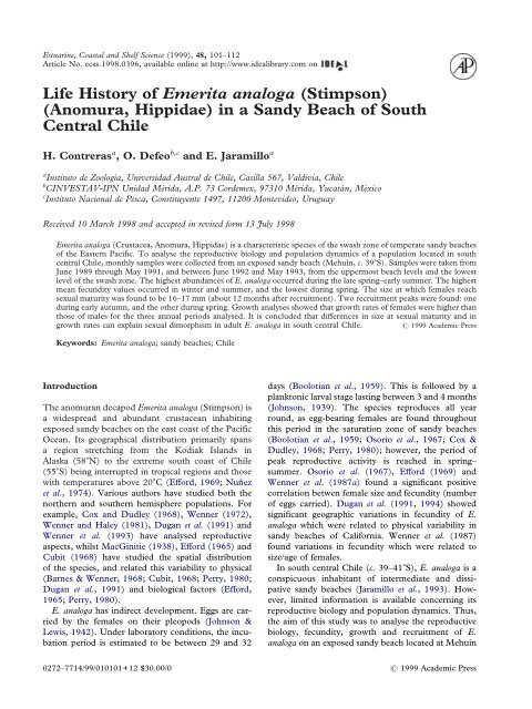
Estuarine, Coastal and Shelf Science (1999), 48, 101–112
Article No. ecss.1998.0396, available online at http://www.idealibrary.com on
Life History of Emerita analoga (Stimpson)
(Anomura, Hippidae) in a Sandy Beach of South
Central Chile
H. Contreras a , O. Defeo b,c and E. Jaramillo a
a Instituto de Zoología, Universidad Austral de Chile, Casilla 567, Valdivia, Chile
b CINVESTAV-IPN Unidad Mérida, A.P. 73 Cordemex, 97310 Mérida, Yucatán, México
c Instituto Nacional de Pesca, Constituyente 1497, 11200 Montevideo, Uruguay
Received 10 March 1998 and accepted in revised form 13 July 1998
Emerita analoga (Crustacea, Anomura, Hippidae) is a characteristic species of the swash zone of temperate sandy beaches
of the Eastern Pacific. To analyse the reproductive biology and population dynamics of a population located in south
central Chile, monthly samples were collected from an exposed sandy beach (Mehuín, c. 39S). Samples were taken from
June 1989 through May 1991, and between June 1992 and May 1993, from the uppermost beach levels and the lowest
level of the swash zone. The highest abundances of E. analoga occurred during the late spring–early summer. The highest
mean fecundity values occurred in winter and summer, and the lowest during spring. The size at which females reach
sexual maturity was found to be 16–17 mm (about 12 months after recruitment). Two recruitment peaks were found: one
during early autumn, and the other during spring. Growth analyses showed that growth rates of females were higher than
those of males for the three annual periods analysed. It is concluded that differences in size at sexual maturity and in
growth rates can explain sexual dimorphism in adult E. analoga in south central Chile. 1999 Academic Press
Keywords: Emerita analoga; sandy beaches; Chile
Introduction
The anomuran decapod Emerita analoga (Stimpson) is
a widespread and abundant crustacean inhabiting
exposed sandy beaches on the east coast of the Pacific
Ocean. Its geographical distribution primarily spans
a region stretching from the Kodiak Islands in
Alaska (58N) to the extreme south coast of Chile
(55S) being interrupted in tropical regions and those
with temperatures above 20C (Efford, 1969; Nuñez
et al., 1974). Various authors have studied both the
northern and southern hemisphere populations. For
example, Cox and Dudley (1968), Wenner (1972),
Wenner and Haley (1981), Dugan et al. (1991) and
Wenner et al. (1993) have analysed reproductive
aspects, whilst MacGinitie (1938), Efford (1965) and
Cubit (1968) have studied the spatial distribution
of the species, and related this variability to physical
(Barnes & Wenner, 1968; Cubit, 1968; Perry, 1980;
Dugan et al., 1991) and biological factors (Efford,
1965; Perry, 1980).
E. analoga has indirect development. Eggs are carried
by the females on their pleopods (Johnson &
Lewis, 1942). Under laboratory conditions, the incubation
period is estimated to be between 29 and 32
days (Boolotian et al., 1959). This is followed by a
planktonic larval stage lasting between 3 and 4 months
(Johnson, 1939). The species reproduces all year
round, as egg-bearing females are found throughout
this period in the saturation zone of sandy beaches
(Boolotian et al., 1959; Osorio et al., 1967; Cox &
Dudley, 1968; Perry, 1980); however, the period of
peak reproductive activity is reached in spring–
summer. Osorio et al. (1967), Efford (1969) and
Wenner et al. (1987a) found a significant positive
correlation betwen female size and fecundity (number
of eggs carried). Dugan et al. (1991, 1994) showed
significant geographic variations in fecundity of E.
analoga which were related to physical variability in
sandy beaches of California. Wenner et al. (1987)
found variations in fecundity which were related to
size/age of females.
In south central Chile (c. 39–41S), E. analoga is a
conspicuous inhabitant of intermediate and dissipative
sandy beaches (Jaramillo et al., 1993). However,
limited information is available concerning its
reproductive biology and population dynamics. Thus,
the aim of this study was to analyse the reproductive
biology, fecundity, growth and recruitment of E.
analoga on an exposed sandy beach located at Mehuín
0272–7714/99/010101+12 $30.00/0 1999 Academic Press

102 H. Contreras et al.
20°
30°
40°
50°
(c. 39S) over a study period long enough to evaluate
temporal variability in these population characteristics.
Material and methods
39°23'
39°25'
39°27'
Study area
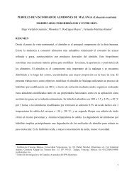
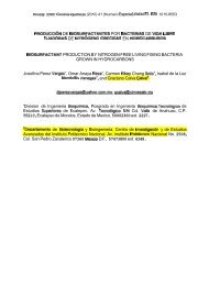
The study beach (c. 200 m long) was located at
Mehuin (3926S, 7313W) on the Valdivian coast,
south–central Chile (Figure 1). The beach is bounded
by rocky promontories consisting primarily of micaceous
schist from which the majority of sand on the
beach is formed (mostly particles between 125 and
250 m, Jaramillo, 1987). Physical factors, such as
wave action, tides, coastal currents and winds significantly
affect the beach’s morphology, which experiences
two marked distinct periods: an erosion period
from mid autumn to early spring and an accretion
period from late spring to early autumn (Jaramillo,
1987).
Sampling and data analysis
From June 1989 to May 1991, monthly samples were
taken during spring tides. Six transects were fixed
perpendicular to the coast, approximately 50 m apart
(Figure 1). Sampling points were situated along each
of these transects at 10 m intervals from the upper
high tide mark to the lower level of the swash zone. As
CHILE
0 1 km
Mehuin '
Sandy beaches
73°12' 73°10'
LLS
LLS: lowest limit of swash
0 30 m
Figure 1. Location of the study area at Mehuín, south central Chile. The six lines on the rectangle of the right side show the
approximate location of the six transects sampled during the period June 1989–May 1991. The lines with asterisks show
the location of the two sampling transects (north and south side of the beach) during the period June 1992–May 1993.
E. analoga has a patchy distribution, this sampling
strategy was followed to obtain a representative
sample of the population on the whole beach. Because
of the seasonal height fluctuations of the beach, the
total number of stations on each transect varied during
the sampling period between 25 and 54 stations
per month, with an average of 39.
Additional samplings were carried out between June
1992 and August 1993. During this period, just two
transects were sampled (north and south ends of the
beach; Figure 1). Ten equidistant sampling points
were arranged along each transect. The second station
was located at the high tide mark and the last at the
lowest swash level. Three 0·03 m 2 replicates were
taken in each of these stations and the animals collected
from each replicate were transferred to the
laboratory for sexing and measurement.
During both sampling periods, the samples were
obtained using a plastic cylinder (20 cm in diameter)
buried to a depth of approximately 25 cm. The sediment
was sieved through a 1000 m mesh and the
animals retained preserved in 10% formalin. Individuals
were measured using the length of the cephalothorax
(thus, Lc=body size) i.e. from the tip of the
rostrum to the distal scoop of the cephalothorax. The
smallest individuals (i.e. Lc

Mean abundance per 0.03 m 2 (X ± 1 s.e.)
60
40
20
0
20
10
0
20
10
0
12
8
4
0
Total
J A O D F A J A O D F A J A O D F A
J A O D F A J A O D F A J A O D F A
J A O D F A J A O D F A J A O D F A
Ovigerous
J A O D F A J A O D F A J A O D F A
80
60
40
20
0
Juveniles
J A O D F A J A O D F A J A O D F A
89
90 91 92 93
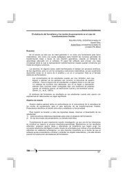
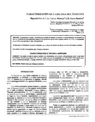
Figure 2. Temporal variability in the abundance of E. analoga during both study periods: June 1989–May 1991 and June
1992–May 1993.
%
%
40
20
0
80
60
40
20
0
J
J
Ovigerous
A O D F A J A O D F A J A O D F A
Juveniles
A O D F A J A O D F A J A O D F A
89
90 91 92
93
Life history of Emerita analoga 103
Figure 3. Temporal variability in the abundance (expressed as percentage of the total population) of ovigerous females and
juveniles of E. analoga during both study periods.

104 H. Contreras et al.
Egg numbers
Egg numbers
Egg numbers
Egg numbers
100 000
10 000
1000
100
10
100 000
10 000
1000
100
10
100 000
10 000
1000
100
10
100 000
10 000
1 15
1 15
1 15
1000
100
10
Winter '89
20 25 30
Spring '89
20 25 30
Summer '90
20 25 30
Autumn '90
1 1
15 20 25 30 35
15 20 25 30 35
Carapace length (mm)
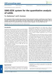
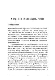
Figure 4. Correlations between the number of eggs and body size of ovigerous females of E. analoga for each seasonal period.
Results of regressions are given in Table 1. Note the logarithm scale in the Y-axis.
males, females without eggs (hereafter females), ovigerous
females and juveniles (i.e. individuals smaller
than 4 mm). Sexes were distinguished on the basis of
anatomical studies carried out by Knox and Boolotian
(1963), Osorio et al. (1967) and Penchaszadeh (1971)
on species of the genus Emerita. Main anatomical
characteristics used were: (1) presence of pleopods
(found exclusively in females); and (2) the genital pore
position, which in females is located in the coxa of the
third pair of pereopods, and in males in the fifth pair.
Juveniles were those whose morphological characters
were absent or difficult to recognize.
35
35
35
Egg numbers
Egg numbers
Egg numbers
Egg numbers
100 000
10 000
1000
100
10
100 000
10 000
1000
100
10
100 000
10 000
1000
100
10
100 000
10 000
1 15
1 15
1 15
1000
100
10
Winter '90
20 25 30
Spring '90
20 25 30
Summer '91
20 25 30
Autumn '91
Fecundity analyses were carried out only for the
period June 1989 to May 1991. The egg mass of each
female was carefully extracted, and the diameters of
10 eggs were measured to estimate their volume
(using the formula for the volume of a sphere). The
total number of eggs in each mass was determined
by displacement of distilled water in a graduated test
tube (0·1 ml accuracy) (Diaz et al., 1983). Fecundity
values were log transformed to calculate regressions
between number of eggs carried by ovigerous females
against body size. Differences of slopes and adjusted
averages among regression lines estimated for each
35
35
35

season were analysed with ANCOVA (Sokal & Rohlf,
1969).
The ELEFAN Program (Electronic Length Frequency
Analysis; see Gayanilo et al., 1989) was
applied to the monthly composition of the population
by sizes, discriminated by sex. The method assumes
that body growth follows the von Bertalanffy Growth
Equation (VGBE) (Bertalanffy, 1938). In its seasonally
oscillating version (Hoenig & Hanumara, 1982)
the VBGE has the form:
Lt=L[1e [K(tt0)+(KC/2)sin2(tts) (KC/2)sin2(t0ts)] ]
where:
Table 1. Seasonal ranges in body size and eggs number carried by ovigerous females. Results of
regression analyses shown in Figure 4 and estimated fecundity for an ovigerous female with
Lc=24·4 mm
Season
L t=length at age t
L=maximum asymptotic length
K=growth curvature parameter
t 0=computed age at length zero
C=parameter reflecting the intensity of seasonal
growth oscillation
t s=start of a sinusoid growth oscillation with respect
to t=0
The Winter Point (WP) parameter is defined as:
WP=t s+0·5
Body size
(range in mm)
or the time (expressed as a decimal fraction of the
year) where growth is slowest (Pauly & Gaschütz,
1979; Pauly et al., 1984).
The ELEFAN program does not assume normality
in the length frequency distributions. It uses the
information on the height and shape of the age distributions
identified in the length frequency data. It
identifies peaks and troughs in the samples and then
fits the growth curve which passes through a maximum
number of peaks (Pauly et al., 1984). An index
Egg numbers
(range) Slope Intercept n r
Life history of Emerita analoga 105
Estimated
fecundity
Winter 1989 20·0–29·7 2879–17 269 0·053 2·60 70 0·68 7808·28
Spring 1989 17·9–30·1 1213–17 746 0·066 2·15 86 0·73 5919·67
Summer 1990 17·8–31·0 1539–24 476 0·074 2·13 90 0·82 8818·45
Autumn 1990 21·2–31·3 979–16 767 0·069 2·07 73 0·67 5639·50
Winter 1990 20·0–31·2 2062–17 277 0·059 2·29 83 0·66 5381·18
Spring 1990 16·0–31·0 691–11 737 0·061 2·16 90 0·73 4524·02
Summer 1991 16·8–31·6 1033–20 374 0·074 2·07 89 0·86 7411·43
Autumn 1991 18·8–30·5 1136–24 731 0·083 1·69 63 0·82 5337·55
of goodness of fit, called Rn, is determined by the
exponential form of the ESP/ASP ratio, where ESP
stands for the ‘ Explained Sum of Peaks ’ and ASP for
‘Available Sum of Peaks ’ as (Gayanilo et al., 1989):
To compare different growth rate estimates, the standard
growth index (phi prime: Pauly & Munro,
1984; Vakily, 1990) was employed as a measure of
overall growth performance (Sparre et al., 1989). This
index is defined as:
=2log 10(L)+log 10K
This rationale provides a unified parameter of growth
performance which does not show large variations as
do K and L values (Sparre et al., 1989). Moreover,
it has been used successfully as a growth index in
bivalves (Vakily, 1990; Defeo et al., 1992a). Thus,
differences in growth performance between sexes and
years were based on comparisons.
The length interval used to carry out the growth
analysis was selected taking into account the criteria
outlined by Wolff (1989) and Sparre (1989). Class
intervals of 2 mm for males and 3 mm for females
were chosen. Longevity was estimated on the basis of
the maximum observed length derived from the relative
age–length key obtained from length–frequency
analyses.
Recruitment pattern was analysed through visual
inspection analyses of histograms and with the estimated
growth parameters, also discriminated by sex,
by projecting the length–frequency data backward
onto the time axis (Pauly et al., 1984; Gayanilo et al.,
1989). As t 0 was not available, the ordinate scale of
the plot was relative, i.e. not calendar time. Normal

106 H. Contreras et al.
Frequency (%)
distribution patterns in recruitment were distinguished
using the maximum likelihood approach
‘ NORMSEP-Hasselblad ’ contained in the FISAT
Program (see Gayanilo et al., 1996 for further details).
Results
45
15
45
15
45
15
45
15
45
15
60
30
45
15
45
15
45
15
45
15
45
15
45
15
1989
45
15
45
15
45
15
45
15
45
15
60
30
45
15
1990 1991
45
15
45
15
45
15
45
15
45
15
1990
0 4 8 12 16 0 4 8 12 16
June
July
August
September
October
November
December
January
February
March
April
May
Body size (mm)
Surf water characteristics
The mean temperature in the surf water was 12·3 C
during the period June 1989 to May 1991, and
12·7 C during June 1992 to May 1993. Values as
high as 15–17 C were registered during summer
45
15
45
15
45
15
45
15
45
15
45
15
45
15
45
15
45
15
45
15
45
15
45
15
1989 1990
45
15
45
15
45
15
45
15
45
15
45
15
45
15
1990 1991
45
15
45
15
45
15
45
15
45
15
0 6 12 18 24 30 0 6 12 18 24 30
August
September
October
November
December
January
February
March
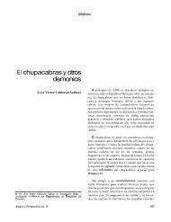
Figure 5. Temporal variability in the population structure of E. analoga during the study period June 1989–May 1991.
June
July
April
May
months, and as low as 10–11 C during winter months
(both study periods compared). During the first study
period, the mean salinity of surf waters was 27·8; for
the second period, a mean of 28·5 was estimated.
Highest salinity values occurred during spring–
summer (up to 31–34) while the lowest usually occurred
during winter months (as low as 18) (both
study periods considered).
Abundance
During the sampling year June 1989 to May 1991,
3326 E. analoga were collected: 1407 males (42·35%);

Frequency (%)
45
15
45
15
45
15
45
15
45
15
45
15
45
15
45
15
45
15
45
15
45
15
45
15
1992
0 4 8 12 16
June
July
August
September
October
November
December
February
March
April
Body size (mm)
1105 females (39·25%); 204 ovigerous females
(6·14%) and 610 juveniles (18·36%). The greatest
abundance of E. analoga was observed during late
spring (November–December of 1989 and December
20
May
45
15
45
15
45
15
45
15
45
15
45
15
45
15
1993 1993
45
January
15
45
15
45
15
45
15
45
15
1992
0 6 12 18 24 30
Life history of Emerita analoga 107
June
July
August
September
October
November
December
January
February
March
Figure 6. Temporal variability in the population structure of E. analoga during the study period June 1992–May 1993.
April
May
of 1990) (Figure 2). Numbers tended to diminish
towards the mid and late summer. During the
sampling year June 1992 to May 1993, 6035 crabs
were collected: 2906 males (46·61%), 2389 females

108 H. Contreras et al.
Table 2. Results of ANCOVA analyses carried out to compare seasonal regression lines describing the relationships between
fecundity and body size of ovigerous females
Source of variation
(38·32%), 97 ovigerous females (1·56%) and 843
juveniles (13·52%); highest abundances during this
period were observed during summer (December–
March) and winter (August) (Figure 2).
Males and females of E. analoga showed their
greatest abundance during December of 1989 and
December of 1992 (Figure 2). During the second
sampling year, males and females were also abundant
during the winter of 1992. Ovigerous females were
collected throughout most of the study periods,
usually in very low abundances (i.e. 2 individuals
per 0·03 m 2 ). The exception was December 1990,
when about 8 ovigerous (mean value) females per
0·03 m 2 were collected. Most of the time, the ratio
of males to females was 1:1, with the exception of
February, July, November of 1990, June, July,
December of 1992 and May of 1993, when significant
differences in this ratio were recorded (P

Frequency (%)
20
10
0
30
15
0
20
10
0
one year
one year
one year
rates always in females as reflected in the growth index
(Figure 8, Table 1). The Winter Point (WP) was
close to 0·5 (excluding only males 1992–1993:
WP=0·8), suggesting a consistent nadir in the growth
curve in June (austral winter) when growth was slowest
for both sexes in both analysed periods. Values of
parameter C were 1·0 in all calculations, implying
heavy seasonal growth oscillations. Female longevity
was nearly 4 years, while for males it was about 2 years
in two of the annual periods analysed.
Discussion
Temporal variability in the abundance of E. analoga at
Mehuín beach showed that the highest abundances
occurred during late spring to early summer and
middle autumn. Those peaks in abundances were
20
10
0
30
15
0
20
10
0
one year
one year
one year
June 1989–May 1990
June 1990–May 1991
June 1992–May 1993
Figure 7. Recruitment pattern of males and females of E. analoga estimated by ELEFAN. The bell shaped curves indicate
the number of recruitment pulses throughout the study period.
Table 3. Estimated growth parameters of Emerita analoga at the beach of Mehuin, south central
Chile, using the ELEFAN Program
Period
Parameters
Life history of Emerita analoga 109
1989–1990 1990–1991 1992–1993
Males Females Males Females Males Females
L (mm) 23·00 34·00 23·00 33·00 26·00 34·00
K (l/yr) 0·48 0·60 0·60 0·80 0·31 0·68
C 1·00 1·00 1·00 1·00 1·00 1·00
WP 0·50 0·52 0·50 0·58 0·80 0·60
2·40 2·84 2·50 2·94 2·32 2·90
Rn a
0·24 0·21 0·52 0·39 0·21 0·27
a Goodness of fit index (explained sum of peaks/available sum of peaks)/10 (see Gayanilo et al., 1989).
primarily related to temporal variability in recruitment,
which peaked at similar periods. Similar results
were found by Jaramillo (1987), who studied the
same beach during 1978–1980. For the coast of
central Chile (Valparaíso, c. 35S) Conan et al. (1975)
also registered two recruitment periods: June and late
September. On the other hand, Osorio et al. (1967)
mentioned one recruitment period during spring for
E. analoga inhabiting a sandy beach in El Tabo (c.
34S), a similar finding to that reported by Efford
(1965) for sandy beaches of California. Thus, variability
in the recruitment pattern of this species along
its extended geographical range seems to be quite
common.
Even though ovigerous females were found all year
round, juveniles were absent or in very low abundances
during some months. That could be related to

110 H. Contreras et al.
Body size (mm)
6 12 18 24 30 36 42
Month
habitat variability as discussed by Dugan et al. (1994)
who found that observed trends in life history of
E. analoga inhabiting sandy beaches of California were
associated with variability in water temperature, food
availability and beach morphodynamics. Significant
changes in beach morphodynamics have been described
for Mehuín (Jaramillo, 1987) which, indeed
might affect the abundance or even presence of
juveniles of E. analoga in the intertidal zone.
The variability in the fecundity of E. analoga has
been related to geographic variability of physical
characteristics of the environment (Dugan et al.,
1991), age classes of females (Wenner et al., 1987a)
and seasonal and local variability of food resources
35
30
25
20
15
10
5
0
35
30
25
20
15
10
5
0
35
30
25
20
15
10
5
0
6 12 18 24 30 36 42
6 12 18 24 30 36 42
48
48
48
June 1989–May 1990
June 1990–May 1991
June 1992–May 1993
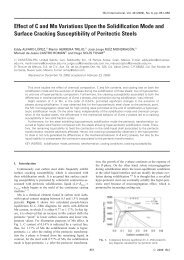
Figure 8. Growth curves of males (solid line) and females (dashed line) of E. analoga estimated by ELEFAN from sets of
length frequency data of June 1989–May 1990, June 1990–May 1991 and June 1992–May 1993.
(Wenner et al., 1987b). However, these studies usually
represent snapshot sampling without annual variability.
The data gathered in this study showed seasonal
variations in fecundity with higher values during
summer months.
Growth rates were fastest for females during the
three annual periods analysed, as reflected by the
highest values of the parameter. Moreover, dissimilar
growth rates between sexes means that longevity of
females would be twice than that of males. Results of
varied slightly between annual periods, denoting
highest growth rates in 1990–1991 for both sexes.
Growth rates varied seasonally in both sexes. Values of
the C parameter were always 1, reflecting intense

seasonal oscillations in growth. In the winter and early
spring months two dissimilar intensities in growth
occurred: growth rate was practically nil during the
winter period and increased abruptly during spring.
These seasonal oscillations suggest that growth in E.
analoga would be affected by temperature differences
between summer and winter in the study area (i.e.
5–6 C). Indeed, growth was minimal from autumn to
late winter (slowest temperatures) and increased
markedly in spring, coinciding with maximum increments
of temperature. It is worth noting that this
relation between temperature and amplitude in the
oscillations of growth (through the parameter C) was
also observed by Arntz et al. (1987), de Alava and
Defeo (1991) and Defeo et al. (1992b) for invertebrates
inhabiting exposed sandy beaches of temperate
latitudes in the Pacific and Atlantic coasts of South
America.
Acknowledgements
We thank Marcia González, Pedro Quijón, Robert
Stead, Sandra Silva, Claudia Añazco, Jacqueline
Muñoz and Sonia Fuentealba for assistance during
field sampling. This study was funded by CONICYT-
CHILE (FONDECYT research projects 88/904 and
92/191) and Universidad Austral de Chile (DID
Project S92/36 and S94/30).
References
Arntz, W. E., Brey, T. T., Tarazona, J. & Robles, A. 1987 Changes
in the structure of a shallow sandy-beach community in Peru
duringanElNiño event. In The Benguela and comparable ecosystems.
(Payne, A. I. L., Gulland, J. A. & Bink, K. H., eds). South
African Journal of Marine Science 5, 645–658.
Barnes, N. B. & Wenner, A. M. 1968 Seasonal variation in the sand
crab Emerita analoga (Decapoda, Hippidae) in the Santa Barbara
area of California. Limnology Oceanography 13, 465–475.
von Bertalanffy, L. 1938 A quantitative theory of organic growth.
Human Biology 10, 181–213.
Boolotian, R. A., Giese, A. C., Farmanfarmalan, A. & Tucker, J.
1959 Reproductive cycles of five west coast crabs. Physiological
Zoology 32, 213–220.
Conan, G., Melo, C. & Yany, G. 1975 Evaluation de la production
d’una population littorale du crabe Hippidae Emerita analoga
(Stimpson) par intégration des paramétres de croissance et de
mortalité. 10th European Symposium on Marine Biology 2, 129–
150.
Cox, G. W. & Dudley, G. H. 1968 Seasonal pattern of reproduction
of the sand crab Emerita analoga, in the Southern California.
Ecology 49, 764–751.
Cubit, J. 1968 Behavior and physical factors causing migration and
aggregation of the sand crab Emerita analoga (Stimpson). Ecology
50, 118–751.
de Alava, A. & Defeo, O. 1991 Distributional pattern and population
dynamics of Excirolana armata (Isopoda: Cirolanidae) in a
Uruguayan sandy beach. Estuarine, Coastal and Shelf Science 33,
433–444.
Life history of Emerita analoga 111
Defeo, O., Arreguín-Sanchez, F. & Sanchez, J. A. 1992a Growth
study of the yellow clam Mesodesma mactroides: a comparative
analysis of the application of three length-based methods. Science
Marine 56, 53–59.
Defeo, O., Ortiz, E. & Castilla, J. C. 1992b Growth, mortality
and recruitment of the yellow clam Mesodesma mactroides in
Uruguayan beaches. Marine Biology 114, 429–437.
Díaz, H., Conde, J. E. & Bevilacqua, M. 1983 A volumetric method
for estimating fecundity in decapoda. Marine Ecology 10, 203–
206.
Dugan, J. E., Hubbard, D. M. & Wenner, A. M. 1991 Geographic
variation in the reproductive biology of the sand crab, Emerita
analoga Stimpson) on the California coast. Journal of Experimental
Marine Biology and Ecology 150, 63–81.
Dugan, J., Wenner, A. M. & Hubbard, D. M. 1994 Geographic
variation in the life history of the sand crab, Emerita analoga
(Stimpson) on the California coast: relationships to environmental
variables. Journal of Experimental Marine Biology and
Ecology 181, 225–278.
Efford, I. E. 1965 Aggregation in the sand crab Emerita analoga
(Stimpson). Ecology 34, 63–75.
Efford, I. E. 1969 Egg size in the sand crab Emerita analoga
(Decapoda, Hippidae). Crustaceana 16, 15–26.
Gayanilo, F. C. Jr., Soriano, M. & Pauly, D. 1989 A draft guide to
the Complete ELEFAN. ICLARM Contribution No 435, 70 pp.
Gayanilo, F. C. Jr., Sparre, P. & Pauly, D. 1996 The FAO-ICLARM
stock assessment tools (FISAT) user’s guide. FAO Computerized
Information Series No 8. Rome, FAO, 126 pp.
Hoenig, J. M. & Hanumara, R. C. 1982 A statistical study of a
seasonal growth model for fishes. Tech. Rep., Dept. of Computer
Science and Statistics, University of Rhode Island, Kingston.
Jaramillo, E. 1987 Community ecology of Chilean sandy beaches.
Ph. D. dissertation University of New Hampshire, Durham,
216 pp.
Jaramillo, E., McLachlan, A. & Coetzee, P. 1993. Intertidal zonation
patterns of macroinfauna over a range of exposed sandy
beaches in south central Chile. Marine Ecology Progress Series 101,
105–118.
Johnson, M. W. 1939 The correlation of water movements and
dispersal of pelagic larval stages of certain littoral animals, especially
the sand crab, Emerita. Journal of Marine Research 11,
236–245.
Johnson, M. W. & Lewis, W. M. 1942 Pelagic larval stages of the
sand crabs Emerita analoga (Stimpson) Blepharipoda occidentalis
(Randall), and Lepidopa myops (Stimpson). Biological Bulletin 83,
67–87.
Knox, C. & Boolotian, R. A. 1963 Functional morphology of
the external appendages of the Emerita analoga. Bulletin of the
Southern California Academy of Science 62, 45–68.
MacGinitie, G. E. 1938 Movements and mating habits of the sand
crab Emerita analoga. American Midland Naturalist 19, 471–481.
Nuñez, J., Aracena, O. & López, M. T. 1974 Emerita analoga en
Llico, provincia de Curicó. (Crustacea, Decapoda, Hippidae).
Boletín de la Sociedad de Biología Concepción 48, 11–22.
Osorio, C., Bahamonde, N. & López, M. T. 1967 El Limanche
[Emerita analoga (Stimpson)] en Chile. Boletín Museo Nacional de
Historia Natural 29, 60–116.
Pauly, D. & Gaschütz, G. 1979 A simple method for fitting
oscillating length growth data, with a program for pocket calculators.
International Council for the Exploration of the Sea Committee
Meeting (Demersal Fish Comm.) 24, 1–26 (mimeo).
Pauly, D., Ingles, J. & Neal, R. 1984 Application to shrimp stocks
of objective methods for the estimation of growth, mortality and
recruitment related parameters from length–frequency data
(ELEFAN I and II). In Penaeid Shrimps, Their Biology and
Management (Gulland, J. A., Rothschild, B. J., eds) Fishing News
Books, Farnham, Surrey, England, 220–234.
Pauly, D. & Munro, J. L. 1984 Once more on the comparison of
growth in fish and invertebrates. Fishbyte 1, 21.
Penchaszadeh, P. 1971 Observaciones cuantitativas en playas
arenosas de la costa central del Perü con especial referencia a

112 H. Contreras et al.
las poblaciones de Muy-Muy (Emerita analoga) (Crustacea,
Anomura, Hippidae). Instituto de Biología Marina–Oficina de
Ciencias de la Unesco 6, 1–19.
Perry, D. M. 1980 Factors influencing aggregation patterns in the
sand crab Emerita analoga (Crustacea, Hippidae). Oecologia 45,
379–384.
Sokal, R. R. & Rohlf, F. J. 1969 Biometria, Madrid, H. Blume,
832 pp.
Sparre, P. 1989 What is the optimum interval class size for
length–frequency analysis? Fishbyte 7, 23.
Sparre, P., Ursin, E. & Venema, S. C. 1989 Introduction to tropical
fish assessment. Part I. Manual. FAO Fish. Tech. Pap. (306.1).
Rome, FAO, 337 pp.
Vakily, J. M. 1990 Determination and comparison of growth
in bivalves, with emphasis on the tropics and Thailand. Ph.D.
Dissertation, Christian- Albrechts–Universität, Germany,
116 pp+Appendix.
Wenner, A. M. 1972 Sex ratio as a function of size in the marine
crustacea. American Naturalist 106, 321–351.
Wenner, A. M. & Haley, S. R. 1981 On the question of sex reversal
in mole crabs (Crustacea, Hippidae). Journal of Crustacean
Biology 1, 506–517.
Wenner, A. M., Richard, Y. & Dugan, J. 1987a Hippid crab
population structure and food availability on Pacific shorelines.
Bulletin of Marine Science 41, 221–233.
Wenner, A. M., Hubbard, D., Dugan, J., Shoffner, J. & Jellison, K.
1987b Egg production by sand crabs (Emerita analoga) as a
function of size and year class (Decapoda, Hippidae). Biological
Bulletin 172, 225–235.
Wenner, A. M., Dugan, J. & Hubbard, D. 1993 Sand crab
population biology on the California Islands and mainland. In
Third California Islands Symposium, Recent Advances in Research on
California Islands (Hochberg, F. G., ed.). Santa Barbara Museum
of Natural History, Santa Barbara, CA, 335–348.
Wolff, M. 1989 A proposed method for standarization of the
selection of class intervals for length frequency analysis. Fishbyte
7, 5.