Kawasaki dynamic in continuum Math. Encounters XXXV ... - CCM

Construction of dynamics Asymptotic Further results
.
Kawasaki dynamic in continuum
Math. Encounters XXXV, Madeira
In honor of
Ludwig Streit
Tobias Kuna
University of Reading
31.7.08
In collaboration with
Yu. G. Kondratiev, M. J. Oliveira, S. L. Silva, L. Streit

Construction of dynamics Asymptotic Further results
Definitions I
Configuration space
Γ := {γ ⊂ R d : |γ ∩ BR(0)| < ∞ for all R},
where BR(0) ball of radius R.
Empirical field
〈f , γ〉 := ∑ f (x)
x∈γ
f = 1
Vol(Λ) 1Λ for Λ ⊂ R d .

Construction of dynamics Asymptotic Further results
Generator
Free Kawasaki dynamics: 0 ≤ a ∈ L 1 (R d )
(LF)(γ) := ∑ x∈γ
dya(x − y) F(γ ∪ {y} \ {x}) − F(γ)
Jump process: Exponential clock with rate a(x)dx;
probability of jump x → y
a(x − y)
a(z)dz
Independent jumps

Construction of dynamics Asymptotic Further results
Independent infinite particle process
Kondratiev, Lytvynov , Röckner: Independent infinite
Markovian particles as an Markov process on the configuration
space
Construct infinite product process on RdN Projection:
R d N
→ Γ
(xn)n∈N ↦→ {xn}n∈N
Corresponding time homogeneous
cadlag Markov process Xt
with law Pγ
for initial value γ ∈ Θ.
Admissible configurations
Θ := γ ∈ Γ : lim sup R
R→∞
−d
|γ ∩ BR(0)| < ∞

Construction of dynamics Asymptotic Further results
Reduction to one particle dynamics
Special class of functions: Bogoliubov exponentials
eB(f )(γ) := ∏(1 + f (x)).
x∈γ
Proper exponential for configuration space
eB(f ) = exp (〈ln(1 + f ), γ〉)
Time development of exponentials
eB(f )(Xt(ω)) Pγ(dω) = eB(e tA f )(γ)
Operator A Markov generator on C∞(Rd )
(Af )(x) := a(y)(f (y + x) − f (x))
R d

Construction of dynamics Asymptotic Further results
Equilibrium dynamics
Initial measure πz with z constant
a symmetric: Dirichlet form, Kondratiev, Lytvynov,
Röckner
Γ
πz(dγ) ∑ x∈γ
2 dya(x − y) F(γ \ x ∪ y) − F(γ)
Second quantization, (also asymmetric). Unique extension.

Construction of dynamics Asymptotic Further results
Local equilibrium dynamics
Poisson random field πz: general intensity 0 ≤ z ∈ L1 loc (Rd )
eB(f )(γ)πz(dγ) = exp f (x)z(x)dx
Γ
Time-development of initial distribution πz
F(γ)Pπz,t(dγ) := F(Xt(ω)) Pγ(dω)πz(dγ)
Solution
with
Pπz,t = πzt
zt := e tA∗
z
Invariant measures: Poisson random fields with constant
intensity z(x) = z0.
Γ

Construction of dynamics Asymptotic Further results
One particle operator
Operator A Markov generator on C∞(Rd )
(Af )(x) := a(y)(f (y + x) − f (x))
R d
Jump process: Exponential clock with rate a(x)dx;
probability of jump x → y
a(x − y)
a(z)dz
Easy form in Fourier variables
Af (k) = (2π) d/2 (â(k) − â(0)) ˆ f (k)
and for the semi-group
e tA f
(x) =
1
(2π) d/2
dke ikx e t(2π)d/2 (â(k)−â(0))ˆ f (k)

Construction of dynamics Asymptotic Further results
Large Time Asymptotic I
Invariant measures:
Pπz,t = πz
Poisson random fields with constant intensity z(x) = z0.
Large time: for t → ∞
lim
t→∞ Pπz,t = lim πzt = πlimt→∞ t→∞
etA∗ z
Reduce to one particle
lim
t→∞
e tA
f (x)z(x)dx = lim
t→∞
e t(2π)d/2 (â(k)−â(0))ˆ f (k)ˆz(k)dk.
Dominated by 1
e t(2π)d/2 (â(k)−â(0)) →
1 if k = 0
0 otherwise

Construction of dynamics Asymptotic Further results
Large Time Asymptotic II
If z ∈ L1 (Rd ) then ˆz(k) ∈ C∞(Rd )
lim e
t→∞
t(2π)d/2
(â(k)−â(0))ˆ f (k)ˆz(k)dk =
{0}
If z := z0 + ∆z with z0 constant ∆z ∈ L 1 (R d ) then
ˆz(k) = z0δ(k) + ∆z(k)
Consequently,
lim e
t→∞
t(2π)d/2 (â(k)−â(0))ˆ f (k)ˆz(k)dk
= ˆf (k) z0δ(k) + ∆z(k) ˆ
dk = z0.
{0}
General argument
ˆz(k)dk signed measure. Then
lim e
t→∞
t(2π)d/2 (â(k)−â(0))ˆ f (k)ˆz(dk)
= ˆf (k)ˆz(dk) = ˆ f (0)ˆz({0}).
{0}
ˆf (k)ˆz(k)dk = 0.

Construction of dynamics Asymptotic Further results
Large Time Asymptotic III
Concluding
lim
t→∞
Define constant by
e tA
f (x)z(x)dx = ˆz({0})
Rd f (x)dx
1
mean(z) := lim
z(x)dx.
R→∞ Vol(BR(0)) BR(0)
∀ϕ ∈ L 1 (R d ) holds
lim
R→∞ R−d
Rd
dxϕ(x/R)z(x) = mean(z)
Rd dxϕ(x)

Construction of dynamics Asymptotic Further results
Large Time Asymptotic IV
∀ϕ ∈ L 1 (R d ) holds
lim
R→∞ R−d
Rd
dxϕ(x/R)z(x) = mean(z)
Rd dxϕ(x)
If ˆz(k)dk signed measure. Then ∀ϕ ∈ L1 (Rd ) holds
lim
= lim
R→∞
Hence
R→∞ R−d
R d
R d
lim
t→∞ Pπz,t = π mean(z).
dxϕ(x/R)z(x)
dx ˆϕ(kR)ˆz(dk) = ˆϕ(0)ˆz({0})

Construction of dynamics Asymptotic Further results
Equilibrium vs. Non-equilibrium, Scales
Equilibrium vs. non-equilibrium
Scales
Equilibrium: πz with z constant
Near equilibrium: density w.r.t. πz with z constant
Local equilibrium: πz with z slowly varying
Far from equilibrium: no density w.r.t any Poisson
measure
System scale: infinity
Space scale (observation)
Time scale (observation)
Interaction scale
Initial data

Construction of dynamics Asymptotic Further results
Examples
Depend only on |x| → ∞.
⎧
0,
⎪⎨ 0,
if z goes to 0
if z ∈ L
mean(z) :=
⎪⎩
p (Rd ), p ∈ [1, 2]
z0,
z0,
z0/2,
if z(x) = z0
if z(x) = z0(1 − α sin(x))
if z(x) = z0 1 (∞,0](x)
Last case: ˆz not signed measure.

Construction of dynamics Asymptotic Further results
General result
Hypothesis:
lim
t→∞ Pπz,t = π mean(z).
if and only if mean(z) exists.
If for z exists tn → ∞ such that
lim e
n→∞
tnA
f (x)z(x)dx
the limit is C f (x)dx.
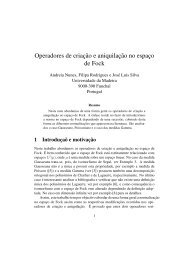
Mean does not exist for all z
z(x) :=
1, if 2 2k ≤ |x| ≤ 2 2k+1
0, otherwise

Construction of dynamics Asymptotic Further results
No overall density
–0.5
1
0.5
0
–1
200 400 600 800 1000
x

Construction of dynamics Asymptotic Further results
Non-equilibrium
Initial measure: µ not Poisson
Cumulants, Ursel functions, truncated moments
ln e 〈f ,γ〉
µ(dγ)
=:
∞
∑
n=1 Rdn n
∏ i=1
(e f (xi) − 1)u (n)
µ (x1, . . . , xn)d dn x
Decay of correlation: some ”mixing condition”
sup
x
∞
∑
k=0
R dk
Density: ρ (1)
µ = u (1)
µ
u (k)
µ ({x, y1, . . . , y k}) dy1 . . . dyn < ∞.

Construction of dynamics Asymptotic Further results
Large time asymptotic
Large times
lim
t→∞ Pµ,t → π mean(ρ (1)
µ )
where
ρ (1)
1
µ := lim
R→∞ Vol(BR(0)) Γ ∑ 1BR(0)(x)µ(dγ). x∈γ
ρµ measure.

Construction of dynamics Asymptotic Further results
Future projects
Time asymptotic for general initial condition
Front propagation: Velocity, Shape
Current
Kawasaki with interaction
Glauber plus Kawasaki
Further variants of interaction