Paper - International Policy Centre for Inclusive Growth

The many dimensions of poverty 

International Conference 

Conference paper 

The many dimensions 

of poverty 

Brasilia, Brazil – 29-31 August 2005 

Carlton Hotel 

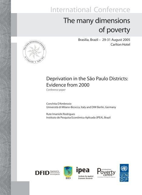
Deprivation in the São Paulo Districts: 

Evidence from 2000 

Conchita D’Ambrosio 

Università di Milano-Bicocca, Italy and DIW Berlin, Germany 

Rute Imanishi Rodrigues 

Instituto de Pesquisa Econômica Aplicada (IPEA), Brazil

Abstract 

Deprivation in the São Paulo Districts: 

Evidence from 2000 ∗ 

Conchita D’Ambrosio 

Università di Milano-Bicocca and DIW Berlin 

conchita.dambrosio@unibocconi.it 

Rute Imanishi Rodrigues 

Instituto de Pesquisa Econômica Aplicada — Government of Brazil 

rute@ipea.gov.br 

July 2005 

This paper aims at capturing the level of deprivation of São Paulo’s population in 2000 

as suffered by its inhabitants in a non-income framework. We construct a measure of 

functioning failure which indicates the degree to which functionings that are considered 

relevant in the city districts are not available to the individuals. Deprivation is measured 

by various indices proposed in the literature: 1) the Yitzhaki, 2) the Esteban and Ray, 

and 3) the Bossert, D’Ambrosio and Peragine indices. Journal of Economic Literature 

Classification No.: D63. 

Keywords: Deprivation, Functionings, Poverty. 

∗ Paper prepared for the International Conference on Multidimensional Poverty, Brasilia, 

29—31 August 2005 organized by the International Poverty Centre, United Nations Development 

Programme.

1 Introduction 

Brazil is often described as the land of inequalities and deprivation is an important issue 

in its metropolitan areas. The city of São Paulo, its richest city in terms of GDP, shows 

striking disparities among its inhabitants (10.4 million in 2000) and worrisome indicators 

of economic well-being. Income inequality is extremely pronounced: while the poorest 

20% possess only 1.5% of total income, the value of the richest 10% is 49%, with a Gini 

coefficient (computed on household per capita income) of 0.62. Beyond income inequality, 

there are more than 2 million living in slums (adding favelas and clandestine lots, see 

Torres, 2003b), almost 9,000 homeless, an unemployment rate higher than 16% since 

2000 (accounting more than 1 million of unemployed in 2003, Seade, 2005b), a general 

mortality rate of 7.04 (rate for 1,000 inhabitants), infant mortality of 16.29 (rate for 1,000 

born alive) per year (See Pardini, 2003) Although more than 90% of children frequent 

primary education, just 54% of teenagers of the city have access to high school, besides 

4.5 % of the adult population is illiterate (Seade, 2005b). Conflict in the city, taking 

homicide rate as indicator, is also extremely high on average, diverging heavily across or 

even within districts: the city homicide rate in 2000 was 57 for 100 thousand inhabitants, 

with this value varying from 4 up to 104 depending on the district (with a standard 

deviation of 24). Although homicide rates are higher in poor districts, in rich and middle 

class neighborhoods homicides are usually extremely high in the favelas placed there (see 

Drumond, 1999). Lethal violence in the city constitutes a serious problem especially for 

the poorest segments of the population, owing to a strong spatial correlation between 

homicide rates and favelas concentration (see Rodrigues, 2005). 

All these facts make of São Paulo a unique case study for deprivation: how does 

someone living in such a city relates to others? The definition of deprivation adopted in 

this paper is that offered by Runciman (1966, p.10): “We can roughly say that [a person] 

is relatively deprived of X when (i) he does not have X; (ii) he sees some other person 

or persons, which may include himself at some previous or expected time, as having X, 

(iii) he sees it as feasible that he should have X”. He further adds: “The magnitude of 

a relative deprivation is the extent of the difference between the desired situation and 

that of the person desiring it”. One of the key variables in measuring deprivation is the 

reference group, that is the group with which a person compares itself. We assume that 

in São Paulo the comparison takes place at the district level: individuals feel that they 

belong to the district where they live and derive within it their standards of comparison 

(See Section 3 for a detailed description). This paper aims at capturing the level of 

1

plight of São Paulo’s population in 2000 analyzing the level of deprivation suffered by its 

inhabitants. 

The measurement of deprivation in a society has traditionally been conducted analyzing 

incomes of individuals, as income summarizes command over resources and is an index 

of the individual’s ability to consume commodities. In this framework a seminal paper 

is that by Yitzhaki (1979) where it is suggested that an appropriate index of aggregate 

deprivation is the absolute Gini index. Hey and Lambert (1980) provide an alternative 

motivation of Yitzhaki’s result. Duclos (2000) shows that a generalization of Gini, the 

class of S-Ginis, could be interpreted as indices of relative deprivation. 

A reason for being interested in deprivation is its representation of the degree of 

discontent or injustice felt by the members of a society. In view of this fact, Podder (1996) 

criticizes the measure of deprivation proposed in the literature and discusses the reasons 

why these are unable to capture the phenomenon. Deprivation and inequality are different 

concepts, hence an index of inequality, such as the Gini coefficient, is inappropriate to 

measure deprivation. In Podder (1996) the distinction between the two is explained by 

their relations to envy. “We say that a person i has a feeling of envy towards person j 

if he prefers to exchange his consumption bundle with that of person j” Podder (1996, 

p.356). Deprivation is proportional to the feeling of envy towards the better off. Equity— 

the absence of inequality—is the absence of envy in all economic agents. At the same 

time, equity coincides with minimum deprivation—all individuals possess the same level 

of income. In constrast, the upper bounds of deprivation and inequality do not coincide. 

Maximum inequality is reached when one individual monopolizes the entire total income; 

maximum deprivation for Podder, on the other hand, is obtained when the society is 

polarized in two equal-sized groups, those possessing income and those not possessing it. 

An analogous distinction with inequality is at the basis of the concept of polarization 

of Esteban and Ray (1994). In a companion paper, Esteban and Ray (1999) link social 

tension and conflict to polarization. The proposed measure of polarization is a variation 

of the Gini coefficient, where not only alienation pays a role, that is the symmetric gaps 

of income that are at the heart of the Gini index, but also identification with identical 

individuals, which is inexistent in the Gini coefficient. Following the Esteban and Ray 

identification/alienation framework, Bossert, D’Ambrosio and Peragine (2005) proposed 

an alternative index of deprivation. (See Section 2 for a detailed description of these 

indices). 

In this paper we compare deprivation in the districts of São Paulo in 2000 using the 

absolute Gini coefficient, the polarization index of Esteban and Ray (1994) and the de- 

2

privation measure of Bossert, D’Ambrosio and Peragine (2005). Since we believe that 

income is not always a good indicator of the command over resources nor of well-being of 

an individual, we follow the suggestion of Bossert, D’Ambrosio and Peragine (2005) and 

compute the indices on deprivation scores based on various functionings. Our exercise 

presents two interesting results. Firstly, the deprivation rankings of districts (by all indices) 

differ from what has been previously reported on São Paulo: we observe a decrease 

in the deprivation position of very poor and homogeneous districts and an increase in 

that of some middle class and rich neighborhoods. This is partially due to the inclusion 

of variables not investigated before, but mainly it is the effect of our choice of indices and 

reference group. Secondly, the rankings of the deprivation index of Bossert, D’Ambrosio 

and Peragine and of that of Esteban and Ray differs from inequality/deprivation ranking 

measured by the absolute Gini coefficient. Even though there is not a clear tendency for 

the divergence, in several cases, if the district is very unequal and fractionalized, Bossert 

D’Ambrosio and Peragine and the Esteban and Ray measure, the latter more intensely 

so, place the district in a lower deprivation position compared to the Gini; the inverse 

occurs if the district is not so unequal but highly polarized. Responsible for these changes 

intherankingsistheidentification component, which is absent in the Gini coefficient. 

The remainder of the paper is organized as follows. The measures of deprivation 

applied in the paper are presented in Section 2. In Section 3, we describe the empirical 

results for Census data for the year 2000. Section 4 concludes. 

2 Measuring deprivation 

In this section we introduce the indices applied to measure deprivation in the São Paulo 

districts. We start with the measure proposed by Bossert, D’Ambrosio and Peragine 

(henceforth BDP, 2005). N denotes the set of all positive integers and R (R+, R++) isthe 

set of all (all non-negative, all positive) real numbers. 

BDP assume that, for each individual, there exists a measure of functioning failure 

which indicates the degree to which functionings that are considered relevant in the society 

under analysis are not available to the agent. The individual functioning failures constitute 

the primary inputs for the analysis and have been predetermined in an earlier stage. A 

natural possibility for such a measure is the number of functioning failures, which is the 

measure used in our empirical application. 

The distinct levels of functioning failures are collected in a vector (q1,..., qK) where 

K ≤ N. Let πj indicate the population share composed of individuals suffering the same 

3

level of functioning failures, qj. Adistributionis(π, q) ≡ (π1, ..., πK; q1, ..., qK), qi 6= qj for 

all i, j ∈ {1, ..., K}. LetΩbethe space of all distributions. q indicates the illfare ranked 

permutationofthevectorq, thatisq1 ≤ q2 ≤ ... ≤ qK. The members of the class of deprivation measures, Di : Ω → R+, characterized by 

BDP are such that the degree of deprivation for a distribution (π,q) is obtained as the 

product of two terms with the following interpretation. The first factor is a multiple 

of the ratio of the number of agents who have fewer functioning failures than i and the 

population size. This number is interpreted as an inverse indicator of agent i’s capacity 

to identify with other members of society—the lack of identification. The second factor is 

the average of the differences between qi and the functioning failures of all agents having 

fewer functionings failure than i. This part captures the aggregate alienation experienced 

by i with respect to those who are better off. In particular the index is defined by: 

Di(π, q) = 

Ã i−1 

X 

j=1 

πj 

! i−1 

X 

(qi − qj)πj, for all (π, q) ∈ Ω. 

This index of individual deprivation incorporates elements of indices proposed earlier in 

the literature of deprivation and polarization. Re-written in terms of functioning failures, 

the individual deprivation suggested by Yitzhaki (1979), a function Ii : Ω → R+, is given 

by: 

Xi−1 

Ii(π, q) = (qi − qj)πj, j=1 

for all (π,q) ∈ Ω, while the effective antagonism introduced by Esteban and Ray (henceforth 

ER, 1994), a function Ai : Ω → R+, is defined as: 

Ai(π, q) =(πi) β 

j=1 

KX 

|qi − qj| πj, 

for all (π, q) ∈ Ω, whereβ∈ [1, 1.6] indicates the degree of polarization sensitivity. In this 

paper we chose β =1; we will assume this parameter value in what follows. 

The three measures share similar elements. Yitzhaki’s measure focuses uniquely on the 

second factor of BDP. Thus, taking into consideration the lack of identification in addition 

to aggregate alienation is what distinguishes the BDP approach from earlier contributions. 

The BDP index resembles that suggested by Esteban and Ray to some extent. However, 

it distinguishes itself from the latter in that it is a measure of deprivation where an 

asymmetry in the alienation component is called for—an individual experiences alienation 

4 

j=1

only with respect to those who are better off. Moreover, a more comprehensive concept of 

identification is required because an individual identifies not only with those like it but, 

instead, with all individuals who are equally well or worse off. 

The BDP aggregate measure of deprivation is a function D: Ω → R+ such that: 

D(π,q) = 

KX 

i=1 

Ã ! 

Xi−1 

Xi−1 

πi πk (qi − qj)πj, k=1 

for all (π, q) ∈ Ω. 

Similarly, aggregate deprivation suggested by Yitzhaki (1979), I: Ω → R+, is given 

by: 

KX Xi−1 

I(π, q) = 

(2) 

i=1 

πi 

j=1 

j=1 

(q i − q j)πj, 

for all (π, q) ∈ Ω, which is equal to the product of the mean of the vector q and the 

Gini coefficient, resulting is the absolute Gini coefficient. In the same way, the effective 

antagonisms felt by all members of the society is total polarization proposed by Esteban 

and Ray (1994), P: Ω → R+, is defined by: 

for all (π, q) ∈ Ω. 

P(π, q) = 

KX 

i=1 

(1) 

KX 

(πi) 2 |qi − qj| πj, (3) 

j=1 

Clearly, the minimal aggregate level of deprivation is equal to zero and attained in 

the case where everyone has the same level of functioning failure, that is, in the case 

of complete equality. This is true for Yitzhaki’s (1979) deprivation index and for BDP 

and ER. In contrast, the maximal level of Yitzhaki’s deprivation index is attained for a 

distribution where one individual has access to all functionings and everyone else has the 

maximal possible functioning failure. Furthermore, ER measure of polarization is maximal 

for a distribution where half of the population have full functioning failure whereas the 

other half have no functioning failures. Interestingly, the BDP aggregate measure of 

deprivation is not maximal for either of those distributions. 

3 The results 

We are not the first to study economic well-being in the districts of São Paulo (see Sposati, 

2000, for an analysis of social exclusion and Seade, 2005a, for vulnerability, just to mention 

5

a few). The present exercise differs in several aspects from previous work: 1) the indices— 

we measure deprivation with Yitzhaki’s index, the ER polarization index, the BDP index; 

2) the reference groups—we assume that the comparison takes place mainly at the district 

level; 3) the functionings analyzed (see below for a discussion). We decide to focus on 

four domains of well-being of an individual, namely: i) living in a secure place with 

access to urban services; ii) attaining the average educational level of its age group; iii) 

having access to a job of minimum quality; iv) having access to the minimum standard 

of consumption of the city. The indices are computed separately for domain i) andforall 

the domains simultaneously. 

We use the following variables from the microdata of the Censo 2000 in order to 

compute individual levels of functionings failures, the qj’s and the associated population 

shares πj’s of the expressions in the previous section (see Table 1 in the Appendix for a 

detailed description of the variables used). 

In particular in domain i) we consider deprived an individual with the following characteristics: 

1. Lives in a rural area. 2. Lives in a favela. 3. Its dwelling is “improvised”. 

4. Its dwelling is of the one-room type. 5. Its dwelling is overcrowded. 6. Lives in a 

polluted area. 7. Lives in a place not served by good urban services. For domains ii) we 

consider deprived the following individuals : 8. Does not have (or has not had) access 

to formal education; for domain iii): 9. Unemployed. or 10. Is a domestic paid worker. 

Finally, for domain iv) deprived is someone who: 11. Does not have access to a minimum 

standard of consumption. 

The individual functioning failure employed in the application is the number, unweighted, 

of the above listed variables that the interviewed claimed to have, or not to 

have, depending on the variable. As a clarifying example for the way we obtain functioning 

failures, consider the variables in the first domain. An individual living in a rural 

area is assigned a score of 1; if, in addition, it lives in a favela it obtains a score of 2; 

if, furthermore, the dwelling is “improvised” then it receives the score 3. And so on for 

all the variables. Once we have obtained these scores for all individuals, we compute the 

population shares associated to the scores for each district separately. In the final step 

we proceede with the calculation of the indices. Keeping the analysis separate at the 

district’s level is driven by our assumption that the comparison takes place at this level: 

individuals feel that they belong to the district where they live and derive within it their 

standards of comparison, as previously explained. Some variables, though, are related to 

the entire city (education of domain ii), labour force status and kind of job of domain iii) 

consumption’s standards of domain iv)). 

6

The first, domain i), seeks to capture the deprivation felt by people living in favelas and 

other kinds of segregated areas characterized by heavy deprivations in terms of housing 

conditions, access to urban services, high level of violence and the social stigma associated 

with it (see Cardia, 2003, Caldeira, 2000). These variables are related to the place of 

residence beyond the conditions of the house in itself. In that, they aim at capturing 

social and environmental aspects of well being such as, for instance, the condition of 

“illegality” and the situation of risk of suffering natural accidents for individuals living 

in favelas (characterized by being an illegal occupation) or clandestine lots (which are 

frequently placed on environmentally protected areas, such as the water source reservoirs 

of Billings and Guarapiranda, Serra da Cantareira forest reserve), where the buildings, 

besides being mostly illegal/irregular, are in addition built in bad terrains (see PMSP, 

2002, Sampaio, 1998, Fernandes, 2003, Torres 2005). Because there are no direct variables 

in the Censo to identify favelas and other kinds of segregated areas, we use the variables 

in Instituto Brasileiro de Geografia eEstatística(IBGE) data that best approximate them 

(see notes on Figure 1 in the Appendix). The relevance given worldwide to this Brazilian 

phenomenon persuaded us to analyze deprivation for this domain separately, as a first 

step of our analysis. 

Domain ii) captures deprivation felt by any person who does not attain the average 

education level within the city for its age group and, in that, it reflects the lower access 

to at least a high school education of people in São Paulo’s periphery (see Seade, 2005b). 

Domain iii) focuses on the deprivation felt by any adult who cannot get a job, or by the 

entire family when the head of the household is unemployed, as well as the low quality of 

jobs offered typically to poor women. For the latter, we focus on domestic workers: this 

group represents around 15% of women’s occupation rate within the city, with values that 

rise to 35% in favelas. At the same time the term “domestic worker” has a symbolical 

meaning: it represents an occupation of the “bottom floor” (see Melo, 1998). The last 

domain iv) is the usual classification of population between poor and non-poor, using a 

poverty line relative to the city income distribution. 

We present the results of our analysis in two steps. First, we discuss the deprivation 

indices applied to the functionings of domain i). Second, we present the overall indices 

and comment on the effect of the inclusion of the remaining variables. To better separate 

the effects captured by the deprivation indices in terms of alienation/identification—that 

is, the interactions between the differences in the functioning failures and the population 

shares—we compare the indices with the sample means of the functioning failures. The 

sample mean, as such, is a purely statistical indicator of the level of deprivation; the 

7

other indices, on the other hand, are derived from behavioral models in the sense that 

they try to capture perceptions of individuals when comparing themselves to others. The 

clearest example to better explain this last point is the following: when the majority of 

the individuals are highly deprived we would observe a high value of the sample mean but 

not of the indices. This is indeed what we observe in our data. 

*Insert Figure 1: Favelas, Rurais and Sample Mean of Variables in Domain i). 

Figure 1 shows how domain i) reflects precariousness of “place of residence”, by comparing 

the localization of favelas (“subnormal sectors”, in IBGE) and areas of environmental 

protection (“rural areas” in IBGE)—at the left side of the figure—with five collections 

of districts grouped according to their sample means of variables in domain i)—at the 

right side of the same figure. In São Paulo precariousness is not exclusively a peripheral 

phenomenon: some districts in the city center that are well served by urban services and 

have no favelas show means relatively high, owing to their proportions of other kinds of 

precarious housing units (like “one-room type” or “improvised” houses, see note on Table 

1 in the Appendix). 

* Insert Figures 2 and 3 

In Figure 2 we plot the rankings obtained from the sample mean against the rankings 

resulting for the deprivation indices, the values being contained in Table 2 in the Appendix. 

1 indicates the lowest value of the index, 96 the highest (since there are 96 districts in 

total). If the indices would produce the same rankings of the sample mean, we would 

observe values lying on the 45o line since we have ordered the districts according to its 

rankings. This is what we observe for a third of our sample, the least deprived districts. 

From the district occupying the 35th position onwards, on the other hand, we observe 

increasing dissimilarities, with the three indices showing similar patters with values being 

on average higher first and lower afterwards. According to behavioral deprivation indices, 

the most deprived districts based on the means of the functionings score would be less 

deprived than those occupying the middle positions. The three behavioral indices applied 

to the functionings of domain i) tend to reduce the importance of deprivation in districts 

with very high sample mean and very low population share having full access, that is the 

individuals showing qj =0. In the extreme south of the city, Marsilac (52), which is the 

worst in the ranking according to the sample mean, jumps to the middle of the orders 

of ER and down to the 35th position according to BDP; similarly, Parelheiros (55) and 

Cidade Tiradentes (25) fall considerably in position; in these districts the population share 

8

with qj =0is zero (in Marsilac) or, almost zero (in Parelheiros and Cidade Tiradentes), 

because they are (totally or almost) rural districts. In Figure 3, we plot the rankings of the 

three deprivation indices relative to the Yitzhaki index. As the figure shows, the rankings 

do not coincide. We confirm values being on average higher first and lower afterwards 

for BDP and ER, modifying Yitzhaki’s rankings. BDP and ER register higher values in 

districts that are extremely polarized (high proportions of population with qj =0and 

qj > 0) and lower values in districts that are homogeneously deprived (very low population 

share with qj =0). Indeed, on the top of the BDP and ER rankings stand districts such 

as Jaguaré (41), where favelas account for around 30% of households while being a middle 

class district. In districts such as Jaguaré, the majority of the population shows the lowest 

qj’s (qj =0) but the highest qj’s (in this case qj ≥ 4) account for big proportions of the 

population. In contrast, Parelheiros (55) goes back to the 62nd position in ER, while 

being among the most deprived according to BDP and Yitzhaki—81 st and 89 th position 

respectively. 

* Insert Figure 4 

Figure 4 gives a spacial view of the differences described above. The districts of the 

city center, where the majority of individuals have complete access, presents the lowest 

values according to all measures, for the others it depends on the index used and on 

the importance given to the alienation component—the heart of the Yitzhaki index—to its 

interaction with identification—in the ER index—to the modification of the latter—in the 

BDP index. 

* Insert Figures 5, 6 and 7 

When we add the other domains, ii) toiv), the overall picture of the results for the 

three indices keep showing the overall tendencies previously commented on for the case 

of domain i) but the differences are now amplified. In Figure 5, the equivalent of Figure 

2, we plot the rankings obtained from the sample mean against the rankings resulting 

for the deprivation indices, the values being contained in Table 3 in the Appendix. The 

rankings now coincide only for very few districts, precisely 17. From that point onwards 

we observe increasing dissimilarities, with the three indices showing similar patters with 

values being on average higher first and lower afterwards, as in the case of domain i), 

but with all the variables jointly considered, the waves are wider. In addition, the indices 

better discriminate the deprivation level of richer districts, particularly so BDP and ER. 

This is partially an effect of the inclusion of “domestic paid workers” as a variable of 

9

deprivation: the richest districts have high proportions of domestic workers, even if part 

of these women live in the house of their employers. The inclusion of the remaining 

variables has the further effect of giving higher scores to individuals already deprived in 

domain i), since to them opportunities of education, job and income tend to be worst. 

Overall BDP and ER reinforce the discrimination of the most polarized and the most 

homogeneous districts (Figure 6 and 7, and Table 3). The comparison of BDP and 

Yitzhaki orders shows that some poor districts in the extreme periphery (mostly in the 

South and the East) are more unequal than deprived due to their homogeneity, as in the 

cases of Marsilac, Parelheiros, Lajeado, Guaianazes and Cidade Tiradentes, which fall 

considerably in the rankings, from Yitzhaki to BDP. On the other hand, some rich and 

middle class districts (mostly in the West zone) are more deprived than unequal due to 

polarization, as Morumbi, Barra Funda, Campo Belo, Vila Sônia and Rio Pequeno, which 

rise considerably in ranking’s position from Yitzhaki to BDP. In the ranking generated 

by ER districts in the extreme periphery are not on top (except for Tremembé, which 

is partially occupied by rich people), but in the middle or even in the lower end of the 

ranking. This is due to the homogeneous deprivation present in these districts. In contrast 

the rich and middle-class districts of the West zone cited above are, together with less 

peripheral districts (including some with very big favelas, as Heliópolis in Sacomã) at the 

top, being the most polarized districts in the city. See Figure 6 for the rankings of the 

three deprivation indices relative to the one generated by Yitzhaki’s. See Figure 7 for a 

spacial view of the differences described above. 

Figure 8 below is an example of polarized and homogeneous districts. The left panel 

represents rich and middle class districts in the Western zone, which have big proportions 

of households in favelas (48% in Vila Andrade, 11% in Morumbi, 27% in Jaguaré, and 

17% in Vila Sônia, 17% in Rio Pequeno). Favelas are represented by ligheter-colored parts 

of the districts, including Paraisópolis, in Vila Andrade, one of the most populated in the 

city. While people from favelas show high scores on deprivation, people outside favelas 

are not deprived at all (or much less deprived)—polarization is high. The panel on the 

right represents districts in the extreme Eastern zone, where there are few households 

in favelas (4% in Lajeado) but where a lot of individuals show high functioning failure 

(for instance, besides income, there are big proportions in “rural” areas, 87% in Cidade 

Tiradentes and 16% in Guaianazes)—these are “homogeneous districts”. 

* insert Figure 8 

10

4 Conclusion 

This paper investigates deprivation as measured by behavioral indices such as the Yitzhaki 

and the Bossert, D’Ambrosio and Peragine deprivation indices and the polarization index 

of Esteban and Ray. As opposed to statistical measures such as sample means, these 

indices allow to capture perceptions of individuals when comparing themselves to others. 

Thus they better identify deprivation of poor individuals living in rich districts, and 

of poor individuals living in poor districts characterized by a homogeneous status of 

deprivation. Polarization and deprivation are important aspects of the Brazilian society, 

particularly so for cities like São Paulo where there is a considerable proportion of people 

“having” but the majority are “have-nots”. 

In this paper we have assumed that the comparison among individuals takes place 

at the district level. Future work will aim at extending the analysis assuming various 

reference groups, such as the entire city, age, education groups. 

References 

[1] Bossert, W. and C. D’Ambrosio (2004), “Reference Groups and Individual Deprivation”, 

CIREQ Working Paper, No. 13-2004. 

[2] Bossert, W, C. D’Ambrosio and V. Peragine (2005), “Deprivation and Social Exclusion,” 

CIREQ Working Paper, No. 2-2004, revised version. 

[3] Caldeira, T.P. (2000), Cidade de Muros: Crime Segregação e Cidadania em São 

Paulo, Editora 34 / Edusp, São Paulo. 

[4] Cardia, N., S. Adorno and F. Poleto (2003), “Homicídio e Violação de Direitos Humanos 

em São Paulo,” Estudos Avançados, 17, 43-73. 

[5] Duclos, J-Y. (2000): “Gini Indices and the Redistribution of Income”, International 

Tax and Public Finance, 7, 141-162. 

[6] Duclos, J.-Y., J.-M. Esteban and D. Ray (2004), “Polarization: Concepts, Measurement, 

Estimation,” Econometrica, 72, 1737—1772. 

[7] Drumond Júnior, M. (1999), “Homicídios e Desigualdades Sociais na Cidade de São 

Paulo: Uma Visão Epidemiológica,” Saúde e Sociedade, 8, 63-81. 

11

[8] Esteban, J.-M. and D. Ray (1994), “On the Measurement of Polarization,” Econometrica, 

62, 819—851. 

[9] Esteban, J.-M. and D. Ray (1999), “Conflict and Distribution,” Journal of Economic 

Theory, 87, 379—415. 

[10] Fernandes, E. (2003), “Perspectivas para a Renovação das Políticas de Legalização 

de Favelas no Brasil,” in Abramo, P. (org.) A Cidade da Informalidade, o desafio das 

cidades lation-americanas, Faperj, Rio de Janeiro. 

[11] Hey, J.D. and P. Lambert (1980): “Relative Deprivation and the Gini Coefficient: 

Comment”, Quarterly Journal of Economics, 95, 567-573. 

[12] Melo, H.P. (1998), “O Serviço Doméstico Remunerado no Brasil: de criadas a trabalhadoras,” 

IPEA Texto para Discussão, No 565. 

[13] Pardini Bicudo Véras, M. (2003), “Brazilian Inequalities: Poverty, Social 

Inclusion and Exclusion in São Paulo,” paper downloadable at 

http://www.brown.edu/Departments/Sociology/faculty/silver/sirs/papers/verasenglish.pdf 

[14] PMSP (2002), Atlas Ambiental do Município de São Paulo, SEMME/ SEMPLA, São 

Paulo, paper downloadable at http://atlasambiental.prefeitura.sp.gov.br 

[15] Podder, N. (1996), “Relative Deprivation, Envy and Economic Inequality,” Kyklos, 

3, 353—376. 

[16] Rodrigues, R.I. (2005), “O Lugar dos Pobres e a Violência na Cidade, um estudo 

para o município de São Paulo,” IPEA, mimeo 

[17] Runciman, W.G. (1966), Relative Deprivation and Social Justice, Routledge, London. 

[18] Sampaio, M.R.A. (1998), “Vida na Favela,” in Sampaio, M.R.A. (org), Habitação e 

Cidade, Fauusp/Fapesp, São Paulo. 

[19] Seade, (2005a), Índice da Vulnerabilidade Juvenil, in 

http://www.seade.gov.br/produtos/ivj/ 

[20] Seade, (2005b), Município de São Paulo, in http://www.seade.gov.br/produtos/msp/ 

12

[21] Sen, A.K. (1973), On Economic Inequality, Oxford University Press, Oxford. 

[22] Sen, A.K. (1985), Commodities and Capabilities, North Holland, Amsterdam. 

[23] Sposati, A. (ed.), (2000), “Mapa da Exclusão - Inclusão Social da Cidade de São 

Paulo - 2000, dinâmica social dos anos 90,” PUC_SP, INPE, Instituto Pólis, São 

Paulo. 

[24] Torres, H., H. Alves, M.A. Oliveira (2005), “São Paulo Peri-Urban Dynamics: Some 

Social Causes and Environmental Consequences,” paper presented in Urban Research 

Symposium 2005, “Land Development, Urban Policy and Poverty Reduction,” IPEA- 

World Bank, Brasília. 

[25] Torres, H.G., E. Marques, M.P. Ferreira and S. Bitar, (2003a), “Pobreza e Espaço: 

Padrões de Segregação em São Paulo,” Estudos Avançados, 47, 97-128. 

[26] Torres, H.G., E. Marques and C. Saraiva (2003b), “Favelas no Município de São 

Paulo: Estimativas de População para 1991, 1996 e 2000”. Revista Brasileira de 

Estudos Urbanos e Regionais, 1, 15-30. 

[27] Yitzhaki, S. (1979), “Relative Deprivation and the Gini Coefficient,” Quarterly Journal 

of Economics, 93, 321—324. 

13

Tables: 

Table 1: Domains of Deprivation and Related Variables. 

Domain Variables x (derived variable) deprivation condition age deprivation score (q) 

i. 1. Does the person live in a rural area? Directly from Census questionarie 1 if yes and 0 if no 

2. Does the person live in a favela? idem 1 if yes and 0 if no 

3. Is the person dwelling "improvised"? 

4. Is the person dwelling of the one-room 

idem 1 if yes and 0 if no 

type? idem 1 if yes and 0 if no 

1 if x>3 or the dwelling is improvised 

5. Is the person dwelling overcrowded? total inhab/bedroom 3 

and 0 if x=8 0 if x>=z and 1 if x=age

Table 2: Deprivation Indices for Domain i) 

district mean(q) Absolute-Gini BDP Polarization 

number name order order index order index order index 

32 Moema 1 0.019 1 0.019 1 0.019 1 0.019 

62 Pinheiros 2 0.027 2 0.026 2 0.026 2 0.026 

45 Jardim Paulista 3 0.034 3 0.033 3 0.032 3 0.032 

60 Perdizes 4 0.04 4 0.039 4 0.038 4 0.039 

90 Vila Mariana 5 0.041 5 0.04 5 0.04 5 0.04 

35 Itaim Bibi 6 0.054 6 0.053 6 0.051 6 0.051 

71 Santo Amaro 7 0.057 7 0.055 7 0.053 7 0.054 

48 Lapa 8 0.065 8 0.062 8 0.06 8 0.061 

26 Consolação 9 0.067 9 0.064 10 0.061 9 0.062 

12 Butantã 10 0.069 10 0.064 9 0.061 10 0.064 

77 Saúde 11 0.075 11 0.072 11 0.069 11 0.069 

69 Santa Cecília 12 0.086 12 0.08 12 0.074 12 0.078 

53 Mooca 13 0.088 13 0.083 13 0.078 13 0.08 

2 Alto de Pinheiros 14 0.089 14 0.086 14 0.083 14 0.082 

70 Santana 15 0.097 15 0.091 16 0.086 16 0.088 

80 Tatuapé 16 0.097 17 0.092 17 0.089 15 0.087 

14 Cambuci 17 0.1 16 0.092 15 0.085 17 0.089 

1 Água Rasa 18 0.121 18 0.109 18 0.099 18 0.105 

7 Bela Vista 19 0.137 19 0.122 19 0.109 19 0.117 

82 Tucuruvi 20 0.141 20 0.126 20 0.113 20 0.12 

51 Mandaqui 21 0.149 21 0.133 22 0.121 21 0.125 

49 Liberdade 22 0.154 22 0.137 23 0.124 22 0.128 

56 Pari 23 0.16 24 0.142 24 0.127 23 0.134 

21 Casa Verde 24 0.164 23 0.139 21 0.119 24 0.136 

16 Campo Grande 25 0.173 27 0.155 29 0.142 25 0.141 

20 Carrão 26 0.175 28 0.156 28 0.141 27 0.143 

86 Vila Guilherme 27 0.175 25 0.15 26 0.131 26 0.142 

91 Vila Matilde 28 0.18 26 0.153 25 0.131 28 0.147 

85 Vila Formosa 29 0.186 29 0.159 27 0.139 29 0.149 

27 Cursino 30 0.196 30 0.168 30 0.147 30 0.154 

79 Socorro 31 0.199 31 0.172 31 0.154 31 0.156 

59 Penha 32 0.218 33 0.189 33 0.168 32 0.169 

29 Freguesia do Ó 33 0.224 32 0.184 32 0.156 33 0.17 

66 República 34 0.231 34 0.198 34 0.173 34 0.177 

8 Belém 35 0.25 37 0.224 40 0.207 37 0.193 

15



40 Jaguara 36 0.263 35 0.217 37 0.185 35 0.192 

72 São Lucas 37 0.264 36 0.222 38 0.194 36 0.193 

15 Campo Belo 38 0.273 42 0.25 46 0.236 45 0.221 

93 Vila Prudente 39 0.284 40 0.243 42 0.218 38 0.205 

88 Vila Leopoldina 40 0.285 43 0.256 47 0.238 44 0.22 

64 Ponte Rasa 41 0.301 41 0.244 41 0.208 39 0.208 

92 Vila Medeiros 42 0.304 39 0.243 39 0.203 40 0.209 

10 Brás 43 0.305 44 0.259 43 0.23 42 0.216 

4 Aricanduva 44 0.306 45 0.261 44 0.232 43 0.218 

78 Sé 45 0.314 38 0.234 36 0.181 41 0.212 

5 Artur Alvim 46 0.324 46 0.276 49 0.246 46 0.226 

9 Bom Retiro 47 0.326 47 0.279 50 0.25 47 0.229 

50 Limão 48 0.354 49 0.284 48 0.242 49 0.232 

34 Ipiranga 49 0.361 51 0.306 52 0.274 51 0.246 

18 Cangaiba 50 0.362 48 0.281 45 0.233 48 0.23 

63 Pirituba 51 0.363 50 0.296 51 0.257 50 0.237 

54 Morumbi 52 0.371 53 0.318 56 0.286 57 0.268 

6 Barra Funda 53 0.393 55 0.33 57 0.29 68 0.285 

47 José Bonifácio 54 0.411 54 0.328 54 0.282 53 0.255 

38 Jabaquara 55 0.448 58 0.362 63 0.315 60 0.273 

74 São Miguel 56 0.449 57 0.342 55 0.284 55 0.26 

65 Raposo Tavares 57 0.467 56 0.341 53 0.275 54 0.26 

95 São Domingos 58 0.496 59 0.371 60 0.305 61 0.276 

24 Cidade Lider 59 0.513 60 0.372 58 0.299 58 0.272 

37 Itaquera 60 0.52 61 0.375 59 0.302 59 0.273 

73 São Mateus 61 0.526 62 0.39 66 0.322 64 0.28 

89 Vila Maria 62 0.539 69 0.43 73 0.373 78 0.308 

68 Sacomã 63 0.541 63 0.394 65 0.321 65 0.281 

28 Ermelino Matarazzo 64 0.567 65 0.398 64 0.315 63 0.28 

76 Sapopemba 65 0.586 67 0.422 69 0.344 71 0.291 

94 Vila Sônia 66 0.587 71 0.457 76 0.39 89 0.332 

84 Vila Curuçá 67 0.607 68 0.426 68 0.342 70 0.29 

31 Guaianases 68 0.653 66 0.416 62 0.313 66 0.281 

46 Jardim São Luís 69 0.66 73 0.459 72 0.368 74 0.301 

36 Itaim Paulista 70 0.661 70 0.449 71 0.353 73 0.295 

39 Jaçanã 71 0.665 76 0.485 78 0.401 83 0.315 

67 Rio Pequeno 72 0.683 79 0.509 82 0.426 91 0.336 

17 Campo Limpo 73 0.684 77 0.49 79 0.401 84 0.316 

16



23 Cidade Dutra 74 0.688 75 0.482 75 0.389 80 0.312 

22 Cidade Ademar 75 0.744 80 0.509 80 0.407 85 0.316 

13 Cachoeirinha 76 0.763 82 0.546 88 0.45 90 0.336 

11 Brasilândia 77 0.768 78 0.492 74 0.379 75 0.301 

19 Capão Redondo 78 0.774 81 0.511 77 0.4 81 0.313 

96 Lajeado 79 0.79 74 0.472 70 0.349 69 0.289 

42 Jaraguá 80 0.792 72 0.458 67 0.333 67 0.283 

57 Parque do Carmo 81 0.809 83 0.551 85 0.444 88 0.326 

87 Vila Jacuí 82 0.873 84 0.586 90 0.468 92 0.338 

41 Jaguaré 83 1,006 92 0.706 96 0.566 96 0.463 

44 Jardim Helena 84 1,026 86 0.595 86 0.447 79 0.31 

61 Perus 85 1,029 87 0.614 89 0.465 86 0.325 

43 Jardim Ângela 86 1,046 85 0.592 83 0.441 76 0.304 

81 Tremembé 87 1,151 93 0.716 94 0.56 93 0.354 

30 Grajaú 88 1,169 88 0.62 87 0.448 77 0.306 

58 Pedreira 89 1,189 91 0.669 91 0.497 87 0.325 

75 São Rafael 90 1,231 94 0.728 93 0.551 94 0.358 

83 Vila Andrade 91 1,378 95 0.741 92 0.53 95 0.362 

25 Cidade Tiradentes 92 1,424 64 0.397 61 0.312 56 0.264 

3 Anhanguera 93 1,458 96 0.751 95 0.561 82 0.313 

33 Iguatemi 94 1,581 90 0.668 84 0.443 72 0.294 

55 Parelheiros 95 1,772 89 0.646 81 0.419 62 0.277 

52 Marsilac 96 2,428 52 0.31 35 0.179 52 0.251 

Source: Authors’ calculations from IBGE-CENSO 2000. 

17

Table 3: Deprivation Indices for all Domains. 



32 Moema 1 0.235 1 0.198 1 0.174 1 0.176 

45 Jardim Paulista 2 0.262 2 0.222 2 0.196 2 0.192 

90 Vila Mariana 3 0.27 3 0.226 3 0.197 3 0.195 

60 Perdizes 4 0.302 4 0.243 4 0.206 4 0.207 

62 Pinheiros 5 0.315 5 0.252 5 0.213 5 0.213 

35 Itaim Bibi 6 0.336 6 0.272 6 0.233 6 0.223 

71 Santo Amaro 7 0.361 7 0.281 7 0.234 7 0.23 

26 Consolação 8 0.373 8 0.292 8 0.245 8 0.237 

2 Alto de Pinheiros 9 0.39 10 0.314 11 0.27 10 0.247 

77 Saúde 10 0.399 9 0.306 9 0.253 9 0.243 

48 Lapa 11 0.446 11 0.323 10 0.256 11 0.253 

12 Butantã 12 0.451 12 0.337 12 0.275 12 0.258 

70 Santana 13 0.464 14 0.344 14 0.279 14 0.262 

69 Santa Cecília 14 0.467 13 0.344 13 0.278 13 0.261 

80 Tatuapé 15 0.479 15 0.351 15 0.283 15 0.265 

53 Mooca 16 0.516 16 0.366 17 0.29 16 0.27 

7 Bela Vista 17 0.537 18 0.39 19 0.317 23 0.28 

49 Liberdade 18 0.55 19 0.403 21 0.329 30 0.284 

14 Cambuci 19 0.567 17 0.375 16 0.284 17 0.271 

15 Campo Belo 20 0.636 33 0.516 44 0.457 90 0.352 

16 Campo Grande 21 0.639 23 0.449 30 0.361 56 0.298 

82 Tucuruvi 22 0.66 21 0.425 20 0.322 29 0.284 

1 Água Rasa 23 0.666 20 0.412 18 0.304 20 0.278 

51 Mandaqui 24 0.692 22 0.448 25 0.344 41 0.29 

79 Socorro 25 0.74 26 0.463 27 0.35 43 0.291 

66 República 26 0.747 30 0.476 31 0.365 53 0.296 

20 Carrão 27 0.749 24 0.457 23 0.341 38 0.288 

21 Casa Verde 28 0.774 25 0.458 22 0.336 32 0.285 

56 Pari 29 0.775 29 0.473 28 0.354 44 0.291 

8 Belém 30 0.781 38 0.536 41 0.433 82 0.322 

88 Vila Leopoldina 31 0.784 39 0.543 42 0.44 86 0.327 

86 Vila Guilherme 32 0.787 28 0.471 26 0.35 39 0.288 

27 Cursino 33 0.794 32 0.504 33 0.388 63 0.302 

85 Vila Formosa 34 0.811 27 0.47 24 0.343 33 0.285 

54 Morumbi 35 0.844 52 0.639 66 0.548 95 0.399 

6 Barra Funda 36 0.846 51 0.639 65 0.546 94 0.394 

18



91 Vila Matilde 37 0.847 31 0.485 29 0.355 36 0.287 

59 Penha 38 0.87 36 0.531 37 0.405 64 0.302 

40 Jaguara 39 0.92 34 0.526 34 0.391 48 0.293 

29 Freguesia do Ó 40 0.936 35 0.53 35 0.392 47 0.293 

93 Vila Prudente 41 0.942 43 0.579 43 0.449 75 0.313 

9 Bom Retiro 42 0.942 46 0.619 51 0.495 87 0.334 

10 Brás 43 0.968 44 0.596 46 0.463 78 0.316 

72 São Lucas 44 0.99 40 0.556 38 0.414 52 0.295 

34 Ipiranga 45 1,001 54 0.649 55 0.519 88 0.338 

78 Sé 46 1,010 37 0.535 32 0.385 35 0.287 

64 Ponte Rasa 47 1,045 41 0.567 39 0.418 45 0.292 

92 Vila Medeiros 48 1,061 42 0.571 40 0.419 46 0.293 

4 Aricanduva 49 1,062 45 0.603 45 0.458 67 0.305 

5 Artur Alvim 50 1,090 48 0.627 49 0.48 72 0.309 

50 Limão 51 1,094 47 0.626 48 0.476 71 0.309 

63 Pirituba 52 1,127 53 0.642 50 0.487 73 0.31 

38 Jabaquara 53 1,163 60 0.718 70 0.567 89 0.34 

18 Cangaiba 54 1,179 49 0.633 47 0.47 62 0.301 

95 São Domingos 55 1,223 58 0.697 59 0.532 81 0.321 

94 Vila Sônia 56 1,225 74 0.8 84 0.645 93 0.384 

47 José Bonifácio 57 1,271 55 0.679 53 0.511 66 0.304 

68 Sacomã 58 1,321 63 0.728 67 0.552 79 0.318 

65 Raposo Tavares 59 1,351 56 0.687 52 0.505 59 0.299 

89 Vila Maria 60 1,361 69 0.762 73 0.593 83 0.322 

24 Cidade Lider 61 1,362 57 0.688 54 0.511 54 0.297 

74 São Miguel 62 1,365 59 0.698 56 0.519 60 0.299 

73 São Mateus 63 1,427 64 0.728 64 0.545 65 0.302 

37 Itaquera 64 1,464 62 0.728 61 0.537 61 0.299 

67 Rio Pequeno 65 1,468 82 0.878 90 0.691 91 0.362 

28 Ermelino Matarazzo 66 1,505 61 0.723 58 0.528 51 0.294 

39 Jaçanã 67 1,509 76 0.824 80 0.632 84 0.324 

76 Sapopemba 68 1,590 67 0.752 68 0.556 50 0.294 

23 Cidade Dutra 69 1,618 78 0.832 77 0.625 77 0.315 

17 Campo Limpo 70 1,637 79 0.834 79 0.629 74 0.311 

46 Jardim São Luís 71 1,663 73 0.791 72 0.582 57 0.298 

84 Vila Curuçá 72 1,699 70 0.769 69 0.562 40 0.29 

22 Cidade Ademar 73 1,725 80 0.85 81 0.635 70 0.308 

13 Cachoeirinha 74 1,733 85 0.894 89 0.681 80 0.318 

19



31 Guaianases 75 1,761 65 0.736 57 0.52 24 0.282 

57 Parque do Carmo 76 1,764 84 0.891 87 0.679 76 0.314 

41 Jaguaré 77 1,775 95 1,077 96 0.848 96 0.431 

42 Jaraguá 78 1,778 68 0.755 63 0.545 28 0.284 

36 Itaim Paulista 79 1,835 72 0.784 71 0.569 34 0.285 

19 Capão Redondo 80 1,838 77 0.828 75 0.604 49 0.294 

11 Brasilândia 81 1,859 75 0.818 74 0.596 42 0.291 

87 Vila Jacuí 82 1,924 87 0.908 88 0.679 68 0.305 

96 Lajeado 83 2,018 71 0.772 62 0.545 19 0.278 

81 Tremembé 84 2,042 93 1,020 94 0.77 85 0.326 

61 Perus 85 2,094 89 0.915 86 0.669 58 0.299 

44 Jardim Helena 86 2,211 83 0.886 82 0.638 31 0.285 

43 Jardim Ângela 87 2,290 81 0.872 78 0.626 25 0.282 

58 Pedreira 88 2,312 91 0.979 91 0.711 55 0.297 

75 São Rafael 89 2,342 94 1,022 93 0.747 69 0.307 

83 Vila Andrade 90 2,352 96 1,136 95 0.82 92 0.378 

30 Grajaú 91 2,402 88 0.912 85 0.647 26 0.283 

3 Anhanguera 92 2,521 92 0.996 92 0.736 37 0.288 

25 Cidade Tiradentes 93 2,558 66 0.743 60 0.536 27 0.284 

33 Iguatemi 94 2,780 90 0.933 83 0.641 21 0.279 

55 Parelheiros 95 3,088 86 0.903 76 0.613 18 0.272 

52 Marsilac 96 3,983 50 0.633 36 0.398 22 0.28 


20

Figures: 

Figure 1: Favelas, Rurais and Sample Mean of Variables in Domain i). 

21

91 

81 

71 

61 

51 

41 

31 

21 

11 

1 

Figure 2: Rankings – Deprivation Indices vs Sample Mean – Domain i) 


Moem a 

Pinheiros 

Jardim Paulista 

Perdizes 

Vila Mariana 

Itaim Bibi 

Santo Amaro 

Lapa 

Consolação 

Butantã 

Saúde 

Santa Cecília 

Mooca 

Alto de Pinheiros 

Santana 

Tatuapé 

Cambuci 

Água Rasa 

Bela Vista 

Tucu ruvi 

Mandaqui 

Liberdade 

Pari 

Casa Verde 

Campo Grande 

Carrão 

Vila Guilherme 

Vila M atilde 

Vila Formosa 

Cursino 

Socorro 

Penha 

Freguesia do Ó 

República 

Belém 

Jaguara 

São Luca s 

Campo Belo 

Vila Pru dente 

Vila Leopoldina 

Ponte Rasa 

Vila M edeiros 

Brás 

Aricanduva 

Sé 

Artur Alvim 

Bom Retiro 

Limão 

Ipiranga 

Cangaiba 

Pirituba 

Morumbi 

Barra Funda 

José B onifá cio 

Jabaquara 

São Miguel 

Raposo Tavares 

São Doming os 

Cidade Lider 

Itaquera 

São Mateus 

Vila M aria 

Sacomã 

Ermelino Matarazzo 

Sapopemba 

Vila Sônia 

Vila Curuçá 

Guaian ases 

Jardim São Luís 

Itaim Paulista 

Jaçanã 

Rio Pequen o 

Campo Limpo 

Cidade Dutra 

Cidade Ademar 

Cachoeirinha 

Brasilândia 

Capão Re dondo 

Lajeado 

Jaraguá 

Parque do Carmo 

Vila Jacuí 

Jaguaré 

Jardim Helena 

Perus 

Jardim Ângela 

Tre membé 

Grajaú 

Pedreira 

São Rafael 

Vila Andrade 

Cidade Tiradentes Anhanguera 

Iguatemi 

Parelheiros 

Marsila c 

22 

mean(q) Yitzhaki BDP ER

91 

81 

71 

61 

51 

41 

31 

21 

11 

1 

Figure 3: Rankings – Deprivation Indices – Domain i) 


Moema 

Pinheiros 


Perdizes 

Vila M ariana 

Itaim Bibi 

Santo Amaro 

Lapa 

Consolação 

Butantã 

Saúde 


Mooca 


Santana 

Cambuci 

Tatuapé 

Água Rasa 

Bela Vista 

Tucuruvi 

Mandaqui 

Liberdade 

Casa Verde 

Pari 


Vila Matilde 

Campo Grande 

Carrão 

Vila Formosa 

Cursino 

Socorro 


Penha 

República 

Jaguara 

São Luca s 

Belém 

Sé 

Vila Medeiros 

Vila Prudente 

Ponte Rasa 

Campo Belo 


Brás 

Aricanduva 

Artur Alvim 

Bom Retiro 

Cangaiba 

Limão 

Pirituba 

Ipiranga 

Marsilac 

Morumbi 

José Bonifácio 

Barra Funda 


São Migu el 

Jabaquara 

São Domingos 

Cidade Lider 

Itaquera 

São Mateus 

Sacomã 

Cidade Tiradentes 


Guaian ases 

Sap opemba 

Vila Curuçá 

Vila M aria 


Vila Sônia 

Jaraguá 


Lajeado 

Cidade Dutra 

Jaçanã 

Campo Limpo 

Brasilândia 

Rio Pequeno 

Cidade Ademar 

Capão Redondo 

Cachoeirinha 


Vila Jacuí 


Jardim Helena 

Perus 

Grajaú 

Parelheiros 

Iguatemi 

Pedreira 

Jaguaré 

Tremembé 

São Rafael 

Vila Andrade 

Anhanguera 

23 

Yitzhaki BDP ER

Figure 4: Groups of Districts Based on Rankings of Deprivation Indices and of the Sample Mean – Domain i) 

24

91 

81 

71 

61 

51 

41 

31 

21 

11 

1 

Figure 5: Rankings – Deprivation Indices vs Sample Mean – All Domains 


Moem a 

Jardim Pa ulista 

Vila M ariana 

Perdizes 

Pinheiros 

Itaim Bibi 

Santo Amaro 

Consolação 


Saú de 

Lapa 

Butantã 

Santana 


Tatuapé 

Mooca 

Bela Vista 

Liberdade 

Cambuci 

Campo Belo 

Campo Grande 

Tucuruvi 

Água Rasa 

Mandaqui 

Socorro 

República 

Carrão 

Casa Verde 

Pari 

Belém 



Cursino 

Vila Formosa 

Morumbi 

Barra Funda 

Vila M atilde 

Penha 

Jaguara 


Vila Prudente 

Bom Retiro 

Brás 

São Luca s 

Ipiranga 

Sé 

Pon te Rasa 

Vila Medeiros 

Aricanduva 

Artur Alvim 

Limão 

Pirituba 

Jabaquara 

Cangaiba 

São Doming os 

Vila Sônia 

José B onifá cio 

Sacomã 


Vila M aria 

Cidade Lider 

São Migu el 

São Mateus 

Itaqu era 

Rio Pequeno 


Jaçanã 

Sapopemba 

Cidade Dutra 

Campo Limpo 


Vila Curuçá 

Cidade Ademar 

Cachoeirinha 

Guaianases 


Jaguaré 

Jaraguá 



Brasilândia 

Vila Jacuí 

Lajeado 

Tre membé 

Perus 

Jardim Helena 

Jardim Ân gela 

Pedreira 

São Rafael 

Vila Andrade 

Grajaú 

Anh anguera 


Iguatemi 

Parelheiros 

Marsilac 

25 

mean(q) Yitzhaki BDP ER

91 

81 

71 

61 

51 

41 

31 

21 

11 

1 

Figure 6: Rankings – Deprivation Indices – All Domains 


Moema 


Vila Mariana 

Perdizes 

Pinheiros 

Itaim Bibi 

Santo Amaro 

Consolação 

Saúde 


Lapa 

Butantã 


Santana 

Tatuapé 

Mooca 

Cambuci 

Bela Vista 

Liberdade 

Água Rasa 

Tucuruvi 

Mandaqui 

Campo Grande 

Carrão 

Casa Verde 

Socorro 

Vila Formosa 


Pari 

República 

Vila Matilde 

Cursino 

Campo Belo 

Jaguara 


Penha 

Sé 

Belém 


São Lucas 

Ponte Rasa 

Vila Medeiros 

Vila Prudente 

Brás 

Aricanduva 

Bom Retiro 

Limão 

Artur Alvim 

Cangaiba 

Marsilac 

Barra Funda 

Morumbi 

Pirituba 

Ipiranga 

José Bonifácio 


Cidade Lider 

São Domingos 

São Miguel 

Jabaquara 


Itaquera 

Sacomã 

São Mateus 

Guaianases 


Sapopemba 

Jaraguá 

Vila Maria 

Vila Curuçá 

Lajeado 



Vila Sônia 

Brasilândia 

Jaçanã 


Cidade Dutra 

Campo Limpo 

Cidade Ademar 


Rio Pequeno 

Jardim Helena 


Cachoeirinha 

Parelheiros 

Vila Jacuí 

Grajaú 

Perus 

Iguatemi 

Pedreira 

Anhanguera 

Tremembé 

São Rafael 

Jaguaré 

Vila Andrade 

26 

Yitzhaki BDP ER

Figure 7: Groups of Districts Based on Rankings of Deprivation Indices and of the Sample Mean – All Domains 

27

Figure 8: Examples of Polarized and Homogeneous Districts. 

28

International Poverty Centre 

SBS – Ed. BNDES, 10º andar 

70076-900 Brasilia DF 

Brazil 

povertycentre@undp-povertycentre.org 

www.undp.org/povertycentre 

Telephone +55 61 2105 5000

Paper - International Policy Centre for Inclusive Growth

You also want an ePaper? Increase the reach of your titles

Delete template?

Save as template?