Quantum Trajectories in Phase Space - Center for Nonlinear Studies ...
Quantum Trajectories in Phase Space - Center for Nonlinear Studies ...
Quantum Trajectories in Phase Space - Center for Nonlinear Studies ...

Create successful ePaper yourself
Turn your PDF publications into a flip-book with our unique Google optimized e-Paper software.
Introduction<br />
Numerical Methodology<br />
Applications<br />
The Husimi Representation<br />
Methodology, Revisited<br />
<strong>Quantum</strong> <strong>Trajectories</strong> <strong>in</strong> <strong>Phase</strong> <strong>Space</strong><br />
Craig C. Martens<br />
Department of Chemistry<br />
University of Cali<strong>for</strong>nia, Irv<strong>in</strong>e<br />
Workshop on <strong>Quantum</strong> <strong>Trajectories</strong><br />
<strong>Center</strong> <strong>for</strong> Nonl<strong>in</strong>ear <strong>Studies</strong>, Los Alamos National Laboratory<br />
Los Alamos, NM, July 27-30, 2008<br />
Craig C. Martens <strong>Quantum</strong> <strong>Trajectories</strong> <strong>in</strong> <strong>Phase</strong> <strong>Space</strong>
Introduction<br />
Numerical Methodology<br />
Applications<br />
The Husimi Representation<br />
Methodology, Revisited<br />
Classical and <strong>Quantum</strong> Time Evolution<br />
Classical<br />
Hamilton’s equations<br />
˙q = ∂H<br />
∂p<br />
˙p = − ∂H<br />
∂q<br />
Classical mechanics vs. quantum mechanics<br />
Wigner representation<br />
Entangled Trajectory Molecular Dynamics<br />
<strong>Quantum</strong><br />
Schröd<strong>in</strong>ger equation<br />
i ∂ψ<br />
∂t = ˆ Hψ<br />
Craig C. Martens <strong>Quantum</strong> <strong>Trajectories</strong> <strong>in</strong> <strong>Phase</strong> <strong>Space</strong>
<strong>Quantum</strong> dynamics<br />
Introduction<br />
Numerical Methodology<br />
Applications<br />
The Husimi Representation<br />
Methodology, Revisited<br />
Classical mechanics vs. quantum mechanics<br />
Wigner representation<br />
Entangled Trajectory Molecular Dynamics<br />
Schröd<strong>in</strong>ger Representation<br />
Ψ<br />
Craig C. Martens <strong>Quantum</strong> <strong>Trajectories</strong> <strong>in</strong> <strong>Phase</strong> <strong>Space</strong>
<strong>Quantum</strong> dynamics<br />
Introduction<br />
Numerical Methodology<br />
Applications<br />
The Husimi Representation<br />
Methodology, Revisited<br />
Ψ<br />
Classical mechanics vs. quantum mechanics<br />
Wigner representation<br />
Entangled Trajectory Molecular Dynamics<br />
Craig C. Martens <strong>Quantum</strong> <strong>Trajectories</strong> <strong>in</strong> <strong>Phase</strong> <strong>Space</strong>
Introduction<br />
Numerical Methodology<br />
Applications<br />
The Husimi Representation<br />
Methodology, Revisited<br />
Classical mechanics vs. quantum mechanics<br />
Wigner representation<br />
Entangled Trajectory Molecular Dynamics<br />
<strong>Quantum</strong> dynamics <strong>in</strong> the Wigner representation<br />
Wigner Function<br />
ρ W<br />
Craig C. Martens <strong>Quantum</strong> <strong>Trajectories</strong> <strong>in</strong> <strong>Phase</strong> <strong>Space</strong>
Introduction<br />
Numerical Methodology<br />
Applications<br />
The Husimi Representation<br />
Methodology, Revisited<br />
Classical mechanics vs. quantum mechanics<br />
Wigner representation<br />
Entangled Trajectory Molecular Dynamics<br />
<strong>Quantum</strong> dynamics <strong>in</strong> the Wigner representation<br />
Apologies to Professor Bohm!<br />
Craig C. Martens <strong>Quantum</strong> <strong>Trajectories</strong> <strong>in</strong> <strong>Phase</strong> <strong>Space</strong>
Introduction<br />
Numerical Methodology<br />
Applications<br />
The Husimi Representation<br />
Methodology, Revisited<br />
Classical mechanics vs. quantum mechanics<br />
Wigner representation<br />
Entangled Trajectory Molecular Dynamics<br />
<strong>Quantum</strong> and Classical Liouville Equation<br />
The quantum Liouville equation:<br />
The classical Liouville equation:<br />
where the Poisson bracket is<br />
∂ ˆρ<br />
i<br />
∂t = [ ˆH, ˆρ]<br />
∂ρ<br />
∂t<br />
= {H, ρ}<br />
{H, ρ} = ∂H ∂ρ ∂ρ ∂H<br />
−<br />
∂q ∂p ∂q ∂p<br />
These are connected by the Correspondence Pr<strong>in</strong>ciple:<br />
[ ˆH, ˆρ] → i{ ˆH, ˆρ} + O( 3 )<br />
Craig C. Martens <strong>Quantum</strong> <strong>Trajectories</strong> <strong>in</strong> <strong>Phase</strong> <strong>Space</strong>
The Wigner Function<br />
Introduction<br />
Numerical Methodology<br />
Applications<br />
The Husimi Representation<br />
Methodology, Revisited<br />
Classical mechanics vs. quantum mechanics<br />
Wigner representation<br />
Entangled Trajectory Molecular Dynamics<br />
A phase space representation of a quantum density operator ˆρ:<br />
ρW (q, p, t) = 1<br />
2π<br />
∞<br />
−∞<br />
< q − y<br />
y<br />
2 |ˆρ(t)|q + 2 > eipy/ dy<br />
For a pure state with wave function ψ(q, t) this becomes<br />
ρW (q, p, t) = 1<br />
2π<br />
∞<br />
−∞<br />
ψ ∗ (q + y<br />
y<br />
2 , t)ψ(q − 2 , t)eipy/ dy<br />
Craig C. Martens <strong>Quantum</strong> <strong>Trajectories</strong> <strong>in</strong> <strong>Phase</strong> <strong>Space</strong>
Introduction<br />
Numerical Methodology<br />
Applications<br />
The Husimi Representation<br />
Methodology, Revisited<br />
Wigner Function Equation of Motion<br />
The quantum Liouville equation aga<strong>in</strong>:<br />
Classical mechanics vs. quantum mechanics<br />
Wigner representation<br />
Entangled Trajectory Molecular Dynamics<br />
∂ ˆρ<br />
i<br />
∂t = [ ˆH, ˆρ]<br />
After some algebra, the Wigner trans<strong>for</strong>m the Liouville equation can be<br />
written as<br />
where<br />
∂ρW<br />
∂t<br />
J(q, η) = i<br />
2π2 p ∂ρW<br />
= −<br />
m ∂q +<br />
∞<br />
−∞<br />
∞<br />
−∞<br />
J(q, p − ξ)ρW (q, ξ, t)dξ<br />
y<br />
y<br />
V (q + 2 ) − V (q − 2 ) e −iηy/ dy<br />
Craig C. Martens <strong>Quantum</strong> <strong>Trajectories</strong> <strong>in</strong> <strong>Phase</strong> <strong>Space</strong>
Introduction<br />
Numerical Methodology<br />
Applications<br />
The Husimi Representation<br />
Methodology, Revisited<br />
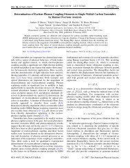
Expression <strong>for</strong> the Kernel J(q, η)<br />
The kernel can be evaluated to give<br />
The result <strong>for</strong> a Gaussian barrier:<br />
Classical mechanics vs. quantum mechanics<br />
Wigner representation<br />
Entangled Trajectory Molecular Dynamics<br />
J(q, η) = 4<br />
<br />
Im ˆV (2η/)e<br />
2 −2iηq/<br />
2<br />
1<br />
0<br />
-1<br />
-2<br />
-10 -5 0 5 10<br />
Craig C. Martens <strong>Quantum</strong> <strong>Trajectories</strong> <strong>in</strong> <strong>Phase</strong> <strong>Space</strong>
Introduction<br />
Numerical Methodology<br />
Applications<br />
The Husimi Representation<br />
Methodology, Revisited<br />
Wigner Function Equation of Motion<br />
Classical mechanics vs. quantum mechanics<br />
Wigner representation<br />
Entangled Trajectory Molecular Dynamics<br />
For a V (q) with a power series expansion J(q, p) becomes<br />
J(q, p) = −V ′ (q) δ ′ (p) + 2<br />
24 V ′′′ (q) δ ′′′ (p) + · · ·<br />
The Wigner function equation of motion is then<br />
∂ρW<br />
∂t<br />
The n th term:<br />
p ∂ρW<br />
= −<br />
m ∂q + V ′ (q) ∂ρW<br />
∂p<br />
(−1) n 2n<br />
2 2n (2n + 1)!<br />
− 2<br />
24 V ′′′ (q) ∂3ρW ∂p<br />
d 2n+1V (q)<br />
dq2n+1 ∂2n+1ρW (q, p)<br />
∂p2n+1 3 + · · ·<br />
Craig C. Martens <strong>Quantum</strong> <strong>Trajectories</strong> <strong>in</strong> <strong>Phase</strong> <strong>Space</strong>
Introduction<br />
Numerical Methodology<br />
Applications<br />
The Husimi Representation<br />
Methodology, Revisited<br />
Classical Liouville Equation<br />
Classical mechanics vs. quantum mechanics<br />
Wigner representation<br />
Entangled Trajectory Molecular Dynamics<br />
Classical Cont<strong>in</strong>uity <strong>in</strong> <strong>Phase</strong> <strong>Space</strong><br />
The classical Liouville equation<br />
∂ρ<br />
∂t<br />
= {H, ρ}<br />
is a cont<strong>in</strong>uity equation <strong>for</strong> <strong>in</strong>compressible flow <strong>in</strong> phase space:<br />
∂ρ<br />
∂t + ∇ ·j = 0<br />
Craig C. Martens <strong>Quantum</strong> <strong>Trajectories</strong> <strong>in</strong> <strong>Phase</strong> <strong>Space</strong>
Introduction<br />
Numerical Methodology<br />
Applications<br />
The Husimi Representation<br />
Methodology, Revisited<br />
The classical cont<strong>in</strong>uity equation:<br />
where<br />
∇ =<br />
∂/∂q<br />
∂/∂p<br />
<br />
∂ρ<br />
∂t = − ∇ ·j = {H, ρ}<br />
j =<br />
∂H/∂p<br />
−∂H/∂q<br />
Classical mechanics vs. quantum mechanics<br />
Wigner representation<br />
Entangled Trajectory Molecular Dynamics<br />
<br />
ρ ∂ ˙q/∂q + ∂ ˙p/∂p = 0<br />
The current j is then the density times the phase space velocity field<br />
<br />
v = j/ρ<br />
˙q ∂H/∂p<br />
= =<br />
˙p −∂H/∂q<br />
Recover<strong>in</strong>g Hamiltion’s equations!<br />
Craig C. Martens <strong>Quantum</strong> <strong>Trajectories</strong> <strong>in</strong> <strong>Phase</strong> <strong>Space</strong>
Introduction<br />
Numerical Methodology<br />
Applications<br />
The Husimi Representation<br />
Methodology, Revisited<br />
Classical mechanics vs. quantum mechanics<br />
Wigner representation<br />
Entangled Trajectory Molecular Dynamics<br />
Solv<strong>in</strong>g the Classical Liouville Equation Us<strong>in</strong>g <strong>Trajectories</strong><br />
Represent the cont<strong>in</strong>uous function ρ(q, p, t) <strong>in</strong> phase space by a discrete<br />
sampl<strong>in</strong>g with N trajectories.<br />
ρ(q, p, t) = 1<br />
N<br />
N<br />
δ(q − qj(t))δ(p − pj(t))<br />
j=1<br />
where qj(t) and pj(t) is the phase space location of the j th trajectory at<br />
time t.<br />
Each member of the ensemble then evolves (<strong>in</strong>dependently) under<br />
Hamilton’s equations.<br />
Craig C. Martens <strong>Quantum</strong> <strong>Trajectories</strong> <strong>in</strong> <strong>Phase</strong> <strong>Space</strong>
Introduction<br />
Numerical Methodology<br />
Applications<br />
The Husimi Representation<br />
Methodology, Revisited<br />
Classical mechanics vs. quantum mechanics<br />
Wigner representation<br />
Entangled Trajectory Molecular Dynamics<br />
<strong>Quantum</strong> Liouville Equation <strong>in</strong> the Wigner Representation<br />
The Wigner function obeys the phase space equation<br />
∂ρW<br />
∂t<br />
p ∂ρW<br />
= −<br />
m ∂q + V ′ (q) ∂ρW<br />
∂p<br />
− 2<br />
24 V ′′′ (q) ∂3ρW ∂p<br />
3 + · · ·<br />
Cast as a cont<strong>in</strong>uity equation (even though ρW can be negative!):<br />
∂ρW<br />
∂t + ∇ ·jW = 0<br />
which def<strong>in</strong>es a quantum current jW :<br />
∇ ·jW = ∂<br />
<br />
p<br />
∂q m ρW<br />
<br />
+ ∂<br />
<br />
−V<br />
∂p<br />
′ (q)ρW + 2<br />
24 V ′′′ (q) ∂2ρW ∂p<br />
<br />
+ · · · 2<br />
Craig C. Martens <strong>Quantum</strong> <strong>Trajectories</strong> <strong>in</strong> <strong>Phase</strong> <strong>Space</strong>
Introduction<br />
Numerical Methodology<br />
Applications<br />
The Husimi Representation<br />
Methodology, Revisited<br />
<strong>Quantum</strong> <strong>Trajectories</strong><br />
Classical mechanics vs. quantum mechanics<br />
Wigner representation<br />
Entangled Trajectory Molecular Dynamics<br />
The quantum current then def<strong>in</strong>es a vector field <strong>in</strong> phase space:<br />
v = jW /ρW<br />
These give a generalization of Hamilton’s equations:<br />
˙q = vq = p<br />
m<br />
˙p = vp = −V ′ (q) + 2<br />
24 V ′′′ (q) 1<br />
ρW<br />
A ρW –dependent Bohmesque “quantum <strong>for</strong>ce”.<br />
∂2ρW + · · ·<br />
∂p2 Craig C. Martens <strong>Quantum</strong> <strong>Trajectories</strong> <strong>in</strong> <strong>Phase</strong> <strong>Space</strong>
Energy Conservation<br />
Introduction<br />
Numerical Methodology<br />
Applications<br />
The Husimi Representation<br />
Methodology, Revisited<br />
Classical mechanics vs. quantum mechanics<br />
Wigner representation<br />
Entangled Trajectory Molecular Dynamics<br />
The quantum trajectories do not conserve energy <strong>in</strong>dividually.<br />
<br />
dH ∂H ∂H p 2 = ˙q + ˙p =<br />
dt ∂q ∂p m 24 V ′′′ (q) 1 ∂<br />
ρ<br />
2 <br />
ρ<br />
+ · · ·<br />
∂p2 Energy is conserved at the ensemble level.<br />
<br />
dH<br />
=<br />
dt<br />
ρ dH<br />
<br />
dqdp =<br />
dt<br />
<br />
p 2 m<br />
24 V ′′′ (q) ∂2ρ + · · ·<br />
∂p2 <br />
dqdp = 0<br />
This non-conservation of <strong>in</strong>dividual trajectory energy allows quantum<br />
effects to be modeled.<br />
Craig C. Martens <strong>Quantum</strong> <strong>Trajectories</strong> <strong>in</strong> <strong>Phase</strong> <strong>Space</strong>
Introduction<br />
Numerical Methodology<br />
Applications<br />
The Husimi Representation<br />
Methodology, Revisited<br />
Classical mechanics vs. quantum mechanics<br />
Wigner representation<br />
Entangled Trajectory Molecular Dynamics<br />
Entangled Trajectory Molecular Dynamics<br />
For the j th trajectory:<br />
˙pj = −V ′ (qj) + 2<br />
24 V ′′′ 1<br />
(qj)<br />
ρW (q1, q2, . . . , pN)<br />
∂ 2 ρW (q1, q2, . . . , pN)<br />
∂p 2<br />
The equations of motion depend not only on the Hamiltonian H(q, p) at<br />
each po<strong>in</strong>t <strong>in</strong> phase space, but on the entire state ρW . This, <strong>in</strong> turn,<br />
depends on the entire ensemble.<br />
The members of the ensemble are thus entangled with each other. The<br />
statistical <strong>in</strong>dependence of ensemble members <strong>in</strong> classical mechanics is<br />
thus lost <strong>for</strong> quantum trajectories!<br />
Craig C. Martens <strong>Quantum</strong> <strong>Trajectories</strong> <strong>in</strong> <strong>Phase</strong> <strong>Space</strong><br />
+ · · ·
Introduction<br />
Numerical Methodology<br />
Applications<br />
The Husimi Representation<br />
Methodology, Revisited<br />
<strong>Trajectories</strong> <strong>in</strong> <strong>Phase</strong> <strong>Space</strong><br />
Classical mechanics vs. quantum mechanics<br />
Wigner representation<br />
Entangled Trajectory Molecular Dynamics<br />
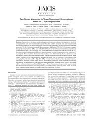
Classical and <strong>Quantum</strong> <strong>Trajectories</strong><br />
p<br />
classical quantum<br />
ρ(q,p,0)<br />
ρ(q,p,t)<br />
q<br />
p<br />
ρ(q,p,0)<br />
ρ(q,p,t)<br />
Classical trajectory ensembles evolve <strong>in</strong>dependently. <strong>Quantum</strong> effects lead to<br />
an entanglement of the ensemble.<br />
Craig C. Martens <strong>Quantum</strong> <strong>Trajectories</strong> <strong>in</strong> <strong>Phase</strong> <strong>Space</strong><br />
q
A Caveat<br />
Introduction<br />
Numerical Methodology<br />
Applications<br />
The Husimi Representation<br />
Methodology, Revisited<br />
Classical mechanics vs. quantum mechanics<br />
Wigner representation<br />
Entangled Trajectory Molecular Dynamics<br />
The Wigner function ρW (q, p, t) is real, but can become negative. Can its<br />
evolution be represented by an ensemble of trajectories evolv<strong>in</strong>g under<br />
these equations of motion?<br />
Craig C. Martens <strong>Quantum</strong> <strong>Trajectories</strong> <strong>in</strong> <strong>Phase</strong> <strong>Space</strong>
Introduction<br />
Numerical Methodology<br />
Applications<br />
The Husimi Representation<br />
Methodology, Revisited<br />
Local Gaussian Ansatz<br />
Numerical Methodology: Local Gaussian Ansatz<br />
An approximate local Gaussian ansatz <strong>for</strong> the Wigner function.<br />
ρ(q, p) = Ae −βq(q−qk) 2 −βp(p−pk) 2 +γ(q−qk)(p−pk)+αq(q−qk)+αp(p−pk)<br />
around the po<strong>in</strong>t k.<br />
Assumption: ρ is on average positive and smooth (<strong>for</strong>malize later).<br />
The parameters αq, αp, βq, βp, and γ are determ<strong>in</strong>ed locally <strong>for</strong> each<br />
member of the ensemble from the moments of the whole ensemble. Then,<br />
1 ∂<br />
ρ<br />
2ρ ∂p2 = α2 p − 2βp<br />
etc.<br />
1 ∂<br />
ρ<br />
4ρ ∂p 4 = α4 p − 12α 2 pβp + 12β 2 p<br />
Craig C. Martens <strong>Quantum</strong> <strong>Trajectories</strong> <strong>in</strong> <strong>Phase</strong> <strong>Space</strong>
Introduction<br />
Numerical Methodology<br />
Applications<br />
The Husimi Representation<br />
Methodology, Revisited<br />
The Trick: Modified Moments<br />
The generator of modified moments is<br />
Ĩ =<br />
∞ ∞<br />
−∞<br />
−∞<br />
Local Gaussian Ansatz<br />
e −βqξ2 −βpη2 +γξη+αqξ+αpη<br />
φhq,hp (ξ, η) dξdη,<br />
where this <strong>in</strong>cludes a local Gaussian w<strong>in</strong>dow function φ:<br />
φhq,hp (ξ, η) = exp −hqξ 2 − hpη 2<br />
The modified m th , n th moment of ξ, η is then<br />
〈ξ ˜ mηn 〉 ≡ 〈ξmηn φ〉<br />
〈φ〉 =<br />
ξ m η n φ(ξ, η)ρ(ξ, η)dξdη<br />
φ(ξ, η)ρ(ξ, η)dξdη<br />
Craig C. Martens <strong>Quantum</strong> <strong>Trajectories</strong> <strong>in</strong> <strong>Phase</strong> <strong>Space</strong>
Modified Moments<br />
Introduction<br />
Numerical Methodology<br />
Applications<br />
The Husimi Representation<br />
Methodology, Revisited<br />
Local Gaussian Ansatz<br />
For ρ a local Gaussian, these moments are generated by derivatives of Ĩ :<br />
〈ξ ˜ mηn 〉 = 1<br />
Ĩ<br />
Generalized variances and correlation:<br />
˜σ 2 ξ<br />
= 〈ξ˜ 2 〉 − ˜ 〈ξ〉 2<br />
∂ (m+n)<br />
∂αm q ∂αn p<br />
˜σ 2 η = ˜ 〈η2 〉 − ˜ 〈η〉 2<br />
Ĩ<br />
˜σ 2 ξη<br />
The orig<strong>in</strong>al Gaussian parameters can then be reconstructed:<br />
αp =<br />
2 ˜σξ 〈η〉 ˜ 2 − σξη ˜ 〈ξ〉 ˜<br />
˜σξ 2 ˜ση 2 − σξη ˜ 4<br />
etc.<br />
βp =<br />
= ˜<br />
〈ξη〉 − ˜<br />
〈ξ〉 ˜<br />
〈η〉<br />
˜σξ 2<br />
2( ˜σξ 2 ˜ση 2 − σξη ˜ 4 )<br />
Craig C. Martens <strong>Quantum</strong> <strong>Trajectories</strong> <strong>in</strong> <strong>Phase</strong> <strong>Space</strong><br />
− hp
Introduction<br />
Numerical Methodology<br />
Applications<br />
The Husimi Representation<br />
Methodology, Revisited<br />
Modified Moments from Ensemble<br />
Local Gaussian Ansatz<br />
The required modified moments can be calculated easily from the evolv<strong>in</strong>g<br />
ensemble:<br />
〈ξ ˜ mηn N j=1<br />
〉 k =<br />
(qj − qk) m (pj − pk) nφ(qj − qk, pj − pk)<br />
N j=1 φ(qj − qk, pj − pk)<br />
This employs local data when determ<strong>in</strong><strong>in</strong>g the local Gaussian fit.<br />
Dist<strong>in</strong>ct parts of the ensemble will be represented by different<br />
Gaussian functions, <strong>in</strong> general.<br />
The method is stable–no NaNs.<br />
In practice, the local w<strong>in</strong>dow function φ is taken to be a m<strong>in</strong>imum<br />
uncerta<strong>in</strong>ty Gaussian. An implicit Husimi representation (see below).<br />
Craig C. Martens <strong>Quantum</strong> <strong>Trajectories</strong> <strong>in</strong> <strong>Phase</strong> <strong>Space</strong>
Introduction<br />
Numerical Methodology<br />
Applications<br />
The Husimi Representation<br />
Methodology, Revisited<br />
Tunnel<strong>in</strong>g Through a Barrier<br />
V(q)<br />
Tunnel<strong>in</strong>g <strong>in</strong> Cubic Potential<br />
Tunnel<strong>in</strong>g <strong>in</strong> a Cubic Potential<br />
0.05<br />
0.04<br />
0.03<br />
0.02<br />
0.01<br />
0<br />
-0.01<br />
-0.02<br />
-1 -0.5 0 0.5 1 1.5<br />
q<br />
p<br />
Craig C. Martens <strong>Quantum</strong> <strong>Trajectories</strong> <strong>in</strong> <strong>Phase</strong> <strong>Space</strong><br />
q
Introduction<br />
Numerical Methodology<br />
Applications<br />
The Husimi Representation<br />
Methodology, Revisited<br />
ETMD <strong>for</strong> Cubic Potential<br />
Tunnel<strong>in</strong>g <strong>in</strong> Cubic Potential<br />
V (q) = 1<br />
2 m ω2 oq 2 − 1<br />
3 bq3<br />
The quantum <strong>for</strong>ce on the j th member of the ensemble:<br />
αp =<br />
˙pj = −V ′ (qj) − 2 b<br />
12<br />
∂ 2 ρ/∂p 2 (qj, pj)<br />
ρ(qj, pj)<br />
˙pj = −V ′ (qj) − 2 b<br />
12 (α2 p,j − 2βp,j)<br />
2 ˜σξ 〈η〉 ˜ 2 − σξη ˜ 〈ξ〉 ˜<br />
˜σξ 2 ˜ση 2 − σξη ˜ 4<br />
βp =<br />
˜σξ 2<br />
2( ˜σξ 2 ˜ση 2 − σξη ˜ 4 )<br />
Craig C. Martens <strong>Quantum</strong> <strong>Trajectories</strong> <strong>in</strong> <strong>Phase</strong> <strong>Space</strong><br />
− hp
Introduction<br />
Numerical Methodology<br />
Applications<br />
The Husimi Representation<br />
Methodology, Revisited<br />
Classical Ensemble <strong>in</strong> <strong>Phase</strong> <strong>Space</strong><br />
p<br />
p<br />
15<br />
10<br />
5<br />
0<br />
-5<br />
-10<br />
-15<br />
15<br />
10<br />
5<br />
0<br />
-5<br />
-10<br />
-15<br />
t = 0<br />
-1 -0.5 0 0.5 1 1.5<br />
q<br />
t = 750<br />
-1 -0.5 0 0.5 1 1.5<br />
q<br />
p<br />
p<br />
Tunnel<strong>in</strong>g <strong>in</strong> Cubic Potential<br />
15<br />
10<br />
5<br />
0<br />
-5<br />
-10<br />
-15<br />
15<br />
10<br />
-5<br />
-10<br />
-15<br />
t = 250<br />
-1 -0.5 0 0.5 1 1.5<br />
q<br />
5<br />
0<br />
-1 -0.5 0 0.5 1 1.5<br />
q<br />
t = 1500 au<br />
Craig C. Martens <strong>Quantum</strong> <strong>Trajectories</strong> <strong>in</strong> <strong>Phase</strong> <strong>Space</strong>
Introduction<br />
Numerical Methodology<br />
Applications<br />
The Husimi Representation<br />
Methodology, Revisited<br />
Entangled Ensemble <strong>in</strong> <strong>Phase</strong> <strong>Space</strong><br />
p<br />
p<br />
15<br />
10<br />
5<br />
0<br />
-5<br />
-10<br />
-15<br />
15<br />
10<br />
t = 0<br />
-1 -0.5 0 0.5 1 1.5<br />
q<br />
5<br />
0<br />
-5<br />
-10<br />
-15<br />
t = 750<br />
-1 -0.5 0 0.5 1 1.5<br />
q<br />
p<br />
p<br />
Tunnel<strong>in</strong>g <strong>in</strong> Cubic Potential<br />
15<br />
10<br />
5<br />
0<br />
-5<br />
-10<br />
-15<br />
15<br />
10<br />
-5<br />
-10<br />
-15<br />
t = 250<br />
-1 -0.5 0 0.5 1 1.5<br />
q<br />
5<br />
0<br />
t = 1500<br />
-1 -0.5 0 0.5 1 1.5<br />
q<br />
Craig C. Martens <strong>Quantum</strong> <strong>Trajectories</strong> <strong>in</strong> <strong>Phase</strong> <strong>Space</strong>
Introduction<br />
Numerical Methodology<br />
Applications<br />
The Husimi Representation<br />
Methodology, Revisited<br />
Tunnel<strong>in</strong>g <strong>in</strong> Cubic Potential<br />
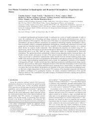
Reaction Probability vs. Time: Classical and Entangled<br />
reaction probability<br />
1<br />
0.8<br />
0.6<br />
0.4<br />
0.2<br />
C3<br />
C2<br />
C1<br />
Q3<br />
Q2<br />
Q1<br />
E1<br />
E3<br />
E2<br />
0<br />
0 1000 2000 3000 4000<br />
time (a.u.)<br />
Craig C. Martens <strong>Quantum</strong> <strong>Trajectories</strong> <strong>in</strong> <strong>Phase</strong> <strong>Space</strong>
Introduction<br />
Numerical Methodology<br />
Applications<br />
The Husimi Representation<br />
Methodology, Revisited<br />
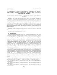
Tunnel<strong>in</strong>g Rate vs. Mean Energy<br />
rate (10 -5 a.u.)<br />
1.4<br />
1.2<br />
1.0<br />
0.8<br />
0.6<br />
0.4<br />
0.2<br />
Tunnel<strong>in</strong>g <strong>in</strong> Cubic Potential<br />
exact quantum<br />
entangled trajectories<br />
0.0<br />
0.00 0.01 0.02 0.03 0.04 0.05<br />
energy (a.u.)<br />
Craig C. Martens <strong>Quantum</strong> <strong>Trajectories</strong> <strong>in</strong> <strong>Phase</strong> <strong>Space</strong>
Eckhart Barrier<br />
Introduction<br />
Numerical Methodology<br />
Applications<br />
The Husimi Representation<br />
Methodology, Revisited<br />
Tunnel<strong>in</strong>g <strong>in</strong> Cubic Potential<br />
The method also captures the quantum corrections to tunnel<strong>in</strong>g through<br />
the Eckhart barrier.<br />
P(t)<br />
0.6<br />
0.5<br />
0.4<br />
0.3<br />
0.2<br />
0.1<br />
Q<br />
E<br />
C<br />
E/V = 0.5<br />
o<br />
0<br />
0 500 1000 1500<br />
t / au<br />
2000 2500 3000<br />
P(t)<br />
0.6<br />
0.5<br />
0.4<br />
0.3<br />
0.2<br />
0.1<br />
Q<br />
E<br />
C<br />
E/V = 0.8<br />
o<br />
0<br />
0 500 1000 1500<br />
t / au<br />
2000 2500 3000<br />
Craig C. Martens <strong>Quantum</strong> <strong>Trajectories</strong> <strong>in</strong> <strong>Phase</strong> <strong>Space</strong><br />
P(t)<br />
0.6<br />
0.5<br />
0.4<br />
0.3<br />
0.2<br />
0.1<br />
Q<br />
E<br />
C<br />
E/V = 1.0<br />
o<br />
0<br />
0 500 1000 1500<br />
t / au<br />
2000 2500 3000
Introduction<br />
Numerical Methodology<br />
Applications<br />
The Husimi Representation<br />
Methodology, Revisited<br />
Husimi Distribution: Positive <strong>Phase</strong> <strong>Space</strong> Distribution<br />
The Husimi Distribution<br />
The Husimi distribution is a locally-smoothed Wigner function:<br />
ρH(q, p) = 1<br />
π<br />
∞<br />
−∞<br />
ρW (q ′ , p ′ )e − (q−q′ ) 2<br />
2σ 2 q e − (p−p′ ) 2<br />
2σ 2 p dq ′ dp ′<br />
where the smooth<strong>in</strong>g is over a m<strong>in</strong>imum uncerta<strong>in</strong>ty phase space Gaussian,<br />
σqσp = <br />
2<br />
Craig C. Martens <strong>Quantum</strong> <strong>Trajectories</strong> <strong>in</strong> <strong>Phase</strong> <strong>Space</strong>
Introduction<br />
Numerical Methodology<br />
Applications<br />
The Husimi Representation<br />
Methodology, Revisited<br />
Operator Formulation of Husimi Distribution<br />
The smooth<strong>in</strong>g can be represented us<strong>in</strong>g smooth<strong>in</strong>g operators ˆQ and ˆP<br />
ˆQ = e 1<br />
2 σ2 q ∂2<br />
∂q 2 ˆP = e 1<br />
2 σ2 p ∂2<br />
∂p 2<br />
The Husimi can then be written as a smoothed Wigner function as:<br />
ρH(q, p) = ˆQ ˆPρW (q, p)<br />
This is related to the <strong>in</strong>terest<strong>in</strong>g identity:<br />
e −a(x−x′ ) 2<br />
∂ 2<br />
= e 1<br />
4a ∂x2 δ(x − x ′ )<br />
Craig C. Martens <strong>Quantum</strong> <strong>Trajectories</strong> <strong>in</strong> <strong>Phase</strong> <strong>Space</strong>
Introduction<br />
Numerical Methodology<br />
Applications<br />
The Husimi Representation<br />
Methodology, Revisited<br />
Smooth<strong>in</strong>g and Unsmooth<strong>in</strong>g<br />
We can consider the <strong>in</strong>verse unsmooth<strong>in</strong>g operators ˆ Q −2 and ˆ P −1 :<br />
ˆQ −1 1<br />
− 2 = e σ2 q ∂2<br />
∂q2 ˆP −1 1<br />
− 2 = e σ2 p ∂2<br />
∂p2 so that the Wigner function can be written (at least <strong>for</strong>mally) as an<br />
“unsmoothed” Husimi:<br />
ρW (q, p) = ˆQ −1 ˆP −1 ρH(q, p)<br />
(Unsmooth<strong>in</strong>g is risky <strong>in</strong> practice, of course!)<br />
Craig C. Martens <strong>Quantum</strong> <strong>Trajectories</strong> <strong>in</strong> <strong>Phase</strong> <strong>Space</strong>
Introduction<br />
Numerical Methodology<br />
Applications<br />
The Husimi Representation<br />
Methodology, Revisited<br />
Equation of Motion <strong>for</strong> the Husimi Distribution<br />
We can then derive an equation of motion <strong>for</strong> the Husimi distribution.<br />
∂ρH 1<br />
= −<br />
∂t m ˆPp ˆP<br />
−1 ∂ρH<br />
∂q +<br />
∞<br />
ˆQJ(q, η) ˆQ −1 ρH(q, p + η, t) dξ<br />
−∞<br />
Note that there are no approximations; the Husimi representation provides<br />
and exact description of quantum dynamics.<br />
Powers of the coord<strong>in</strong>ates and momenta become differential operators:<br />
ˆQq ˆQ −1 = q + σ 2 q<br />
∂<br />
∂q<br />
ˆQq 2 Qˆ −1 2 2<br />
= q + σq + 2σ 2 qq ∂<br />
∂q + σ4 q<br />
ˆPp ˆP −1 = p + σ 2 p<br />
∂2 ∂q2 etc.<br />
Craig C. Martens <strong>Quantum</strong> <strong>Trajectories</strong> <strong>in</strong> <strong>Phase</strong> <strong>Space</strong><br />
∂<br />
∂p
Introduction<br />
Numerical Methodology<br />
Applications<br />
The Husimi Representation<br />
Methodology, Revisited<br />
Equation of Motion <strong>for</strong> the Husimi Distribution<br />
Wigner function equation of motion:<br />
∂ρW<br />
∂t<br />
Husimi equation of motion:<br />
∂ρH<br />
∂t<br />
where<br />
p ∂ρW<br />
= −<br />
m ∂q + (mω2 oq − bq 2 ) ∂ρW<br />
∂p + 2b 12<br />
∂ 3 ρW<br />
∂p 3<br />
1<br />
= −<br />
m ˆ Pp ˆ −1 ∂ρH<br />
P<br />
∂q + (mω2 o ˆ Qq ˆ Q −1 − b ˆ Qq 2 ˆQ −1 ) ∂ρH<br />
∂p + 2b ∂<br />
12<br />
3ρH ∂p3 ˆQq ˆQ −1 = q + σ 2 q<br />
∂<br />
∂q<br />
ˆQq 2 ˆQ −1 = q 2 + σ 2 q + 2σ 2 qq ∂<br />
∂q + σ4 q<br />
ˆPp ˆP −1 = p + σ 2 p<br />
∂2 ∂q2 Craig C. Martens <strong>Quantum</strong> <strong>Trajectories</strong> <strong>in</strong> <strong>Phase</strong> <strong>Space</strong><br />
∂<br />
∂p
Introduction<br />
Numerical Methodology<br />
Applications<br />
The Husimi Representation<br />
Methodology, Revisited<br />
Cont<strong>in</strong>uity <strong>in</strong> the Husimi Representation<br />
We aga<strong>in</strong> <strong>in</strong>voke cont<strong>in</strong>uity, now rigorous <strong>for</strong> a positive probability<br />
distribution.<br />
∂ρH<br />
∂t + ∇ ·jH = 0<br />
Then after a little algebra,<br />
∇ ·jH = ∂<br />
<br />
p<br />
∂q m ρH<br />
<br />
+ ∂<br />
<br />
−V<br />
∂p<br />
′ (q)ρH + b<br />
2mωo<br />
ρH + bq ∂ρH<br />
mωo ∂q + 2b 4m2ω2 ∂<br />
o<br />
2ρH ∂q2 − 2b 12<br />
Craig C. Martens <strong>Quantum</strong> <strong>Trajectories</strong> <strong>in</strong> <strong>Phase</strong> <strong>Space</strong><br />
∂2ρH ∂p2
Introduction<br />
Numerical Methodology<br />
Applications<br />
The Husimi Representation<br />
Methodology, Revisited<br />
<strong>Phase</strong> <strong>Space</strong> Vector Field <strong>in</strong> the Husimi Representation<br />
The phase space vector field then becomes<br />
˙p = −V ′ (q) + b<br />
2mωo<br />
+ bq<br />
mωo<br />
1<br />
ρH<br />
˙q = p<br />
m<br />
∂ρH<br />
∂q + 2 b<br />
4m 2 ω 2 o<br />
1<br />
ρH<br />
∂2ρH ∂q2 − 2b 12<br />
The quantum <strong>for</strong>ce now conta<strong>in</strong>s additional terms not present <strong>in</strong> the<br />
Wigner representation quantum <strong>for</strong>ce. This is related to the fact that<br />
classical propagation and smooth<strong>in</strong>g do not commute.<br />
These equations of motion can be propagated as be<strong>for</strong>e.<br />
Craig C. Martens <strong>Quantum</strong> <strong>Trajectories</strong> <strong>in</strong> <strong>Phase</strong> <strong>Space</strong><br />
1<br />
ρH<br />
∂ 2 ρH<br />
∂p 2
Introduction<br />
Numerical Methodology<br />
Applications<br />
The Husimi Representation<br />
Methodology, Revisited<br />
Free Particle <strong>in</strong> the Husimi Representation<br />
Because of the smooth<strong>in</strong>g, the free particle motion is nonclassical!<br />
or<br />
∂ρH<br />
∂t<br />
∂ρH<br />
∂t<br />
1<br />
= −<br />
m ˆ Pp ˆ −1 ∂ρH<br />
P<br />
∂q<br />
1 ∂ρH<br />
= − p<br />
m ∂q − σ2 p ∂<br />
m<br />
2ρH ∂q∂p<br />
The extra terms due to noncommutativity of classical time evolution and<br />
smooth<strong>in</strong>g.<br />
Craig C. Martens <strong>Quantum</strong> <strong>Trajectories</strong> <strong>in</strong> <strong>Phase</strong> <strong>Space</strong>
Introduction<br />
Numerical Methodology<br />
Applications<br />
The Husimi Representation<br />
Methodology, Revisited<br />
Free Particle Propagation: Entangled vs. Exact<br />
p<br />
7.5<br />
5.0<br />
2.5<br />
0<br />
-2.5<br />
-5.0<br />
t = 1000<br />
(b)<br />
(a)<br />
-2 -1 0 1 2<br />
q<br />
ontour l<strong>in</strong>es of a free particle distribution function <strong>in</strong> the Husimi representation<br />
Craig C. Martens <strong>Quantum</strong> <strong>Trajectories</strong> <strong>in</strong> <strong>Phase</strong> <strong>Space</strong>
Introduction<br />
Numerical Methodology<br />
Applications<br />
The Husimi Representation<br />
Methodology, Revisited<br />
Solv<strong>in</strong>g the Integrodifferential Equation Directly<br />
The Wigner equation of motion:<br />
∂ρW<br />
∂t<br />
Methodology, Revisited<br />
p ∂ρW<br />
= −<br />
m ∂q +<br />
∞<br />
−∞<br />
J(q, p − ξ)ρW (q, ξ, t)dξ<br />
Write the divergence of the flux directly <strong>in</strong> this <strong>for</strong>m:<br />
∇ ·jW = ∂<br />
<br />
p<br />
∂q m ρW<br />
<br />
−<br />
∞<br />
−∞<br />
J(q, ξ − p) ρW (q, ξ, t) dξ<br />
Craig C. Martens <strong>Quantum</strong> <strong>Trajectories</strong> <strong>in</strong> <strong>Phase</strong> <strong>Space</strong>
Introduction<br />
Numerical Methodology<br />
Applications<br />
The Husimi Representation<br />
Methodology, Revisited<br />
Solv<strong>in</strong>g the Integrodifferential Equation Directly<br />
The momentum component:<br />
or<br />
where<br />
∂<br />
∂p jW ,p = −<br />
jW ,p = −<br />
∞<br />
−∞<br />
∞<br />
−∞<br />
Θ(q, ξ − p) ≡<br />
J(q, ξ − p) ρW (q, ξ, t) dξ<br />
Θ(q, ξ − p) ρW (q, ξ, t) dξ<br />
p<br />
−∞<br />
J(q, ξ − z) dz<br />
Craig C. Martens <strong>Quantum</strong> <strong>Trajectories</strong> <strong>in</strong> <strong>Phase</strong> <strong>Space</strong>
Introduction<br />
Numerical Methodology<br />
Applications<br />
The Husimi Representation<br />
Methodology, Revisited<br />
Solv<strong>in</strong>g the Integrodifferential Equation Directly<br />
This can be written explicitly <strong>in</strong> terms of the potential V (q):<br />
Θ(q, ξ − p) = 1<br />
2π<br />
∞<br />
−∞<br />
y<br />
y<br />
V (q + 2 ) − V (q − 2 ) e−i(ξ−p)y/ y<br />
Then the quantum trajectory equations of motion become<br />
<br />
1<br />
˙p = −<br />
ρW (q, p)<br />
˙q = p<br />
m<br />
Θ(q, p − ξ)ρW (q, ξ) dξ<br />
Craig C. Martens <strong>Quantum</strong> <strong>Trajectories</strong> <strong>in</strong> <strong>Phase</strong> <strong>Space</strong><br />
dy
Numerical Approach<br />
Introduction<br />
Numerical Methodology<br />
Applications<br />
The Husimi Representation<br />
Methodology, Revisited<br />
To proceed numerically, we write the Wigner function as a superposition of<br />
Gaussians:<br />
ρW (q, p, t) = 1<br />
N<br />
φ(q − qj(t), p − pj(t))<br />
N<br />
where<br />
j=1<br />
1<br />
φ(q, p) =<br />
2πσqσp<br />
<br />
exp − q2<br />
2σ2 −<br />
q<br />
p2<br />
2σ2 <br />
p<br />
Craig C. Martens <strong>Quantum</strong> <strong>Trajectories</strong> <strong>in</strong> <strong>Phase</strong> <strong>Space</strong>
Numerical Approach<br />
Introduction<br />
Numerical Methodology<br />
Applications<br />
The Husimi Representation<br />
Methodology, Revisited<br />
After some algebra, we f<strong>in</strong>d<br />
˙p(q, p) = −<br />
N<br />
j=1 φq(q − qj)Λ(q − qj, p − pj)<br />
N<br />
j=1 φq(q − qj)φp(q − qj)<br />
where<br />
<br />
V (q + z/2) − V (q − z/2)<br />
Λ(q−qj, p−pj) =<br />
exp i<br />
z<br />
(p − pj)z<br />
<br />
This can be evaluated numerically <strong>for</strong> a given potential V (q).<br />
Craig C. Martens <strong>Quantum</strong> <strong>Trajectories</strong> <strong>in</strong> <strong>Phase</strong> <strong>Space</strong><br />
− σ2 pz 2<br />
22 <br />
dz
Introduction<br />
Numerical Methodology<br />
Applications<br />
The Husimi Representation<br />
Methodology, Revisited<br />
Reaction Probability vs. Time: Classical and Entangled<br />
This method gives better long-time agreement <strong>for</strong> the cubic system:<br />
Reaction probability<br />
1<br />
0.8<br />
0.6<br />
0.4<br />
0.2<br />
Eo=2Vo<br />
Eo=1.25Vo<br />
Eo=0.75Vo<br />
0<br />
0 1000 2000<br />
Time (a.u.)<br />
3000 4000<br />
(Black=exact, red=old method, blue=new method.)<br />
Craig C. Martens <strong>Quantum</strong> <strong>Trajectories</strong> <strong>in</strong> <strong>Phase</strong> <strong>Space</strong>
Conclusions<br />
Introduction<br />
Numerical Methodology<br />
Applications<br />
The Husimi Representation<br />
Methodology, Revisited<br />
It is possible to def<strong>in</strong>e quantum trajectories <strong>in</strong> a non-Bohmian phase<br />
space context.<br />
The phase space quantum trajectory <strong>for</strong>malism can give nearly<br />
quantitative results <strong>for</strong> manifestly quantum mechanical processes such<br />
as tunnel<strong>in</strong>g <strong>in</strong> model systems.<br />
The methodology gives an appeal<strong>in</strong>g picture of quantum processes.<br />
For <strong>in</strong>stance, tunnel<strong>in</strong>g is accomplished by borrow<strong>in</strong>g, not by<br />
burrow<strong>in</strong>g.<br />
Craig C. Martens <strong>Quantum</strong> <strong>Trajectories</strong> <strong>in</strong> <strong>Phase</strong> <strong>Space</strong>
Introduction<br />
Numerical Methodology<br />
Applications<br />
The Husimi Representation<br />
Methodology, Revisited<br />
Mortgage Crisis <strong>in</strong> <strong>Phase</strong> <strong>Space</strong>?<br />
Craig C. Martens <strong>Quantum</strong> <strong>Trajectories</strong> <strong>in</strong> <strong>Phase</strong> <strong>Space</strong>
Acknowledgments<br />
Thanks to:<br />
Introduction<br />
Numerical Methodology<br />
Applications<br />
The Husimi Representation<br />
Methodology, Revisited<br />
⋆ Dr. Arnaldo Donoso (IVIC, Caracas, Venezuela)<br />
Prof. Yujun Zheng (Shandong University)<br />
Jacob Goldsmith<br />
Patrick Hogan<br />
Adam Van Wart<br />
Supported by the<br />
National Science Foundation<br />
Craig C. Martens <strong>Quantum</strong> <strong>Trajectories</strong> <strong>in</strong> <strong>Phase</strong> <strong>Space</strong>