Introduction to numerical processing in Python using Spyder
Introduction to numerical processing in Python using Spyder
Introduction to numerical processing in Python using Spyder

Create successful ePaper yourself
Turn your PDF publications into a flip-book with our unique Google optimized e-Paper software.
<strong>Introduction</strong> <strong>to</strong> <strong>numerical</strong> <strong>process<strong>in</strong>g</strong> <strong>in</strong><br />
<strong>Python</strong> us<strong>in</strong>g <strong>Spyder</strong><br />
Overview<br />
Effective use of programm<strong>in</strong>g <strong>in</strong> scientific research<br />
20 June 2011<br />
School of Civil Eng<strong>in</strong>eer<strong>in</strong>g and Geosciences<br />
Newcastle University<br />
http://conferences.ncl.ac.uk/sciprog<br />
http://www.vitae.ac.uk/programm<strong>in</strong>gforscientists<br />
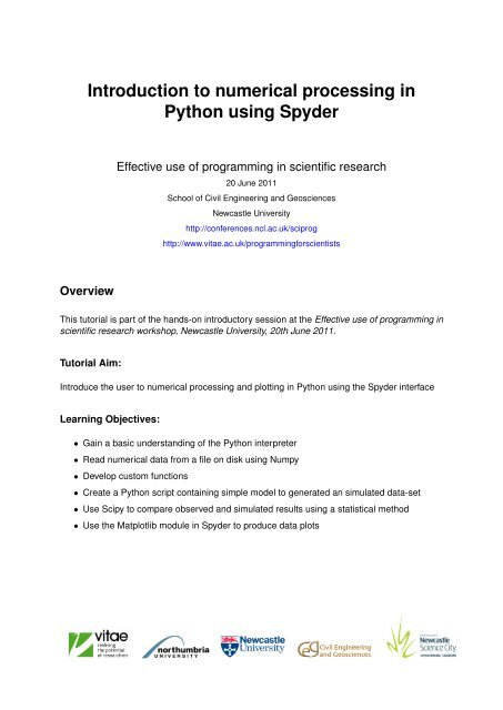
This tu<strong>to</strong>rial is part of the hands-on <strong>in</strong>troduc<strong>to</strong>ry session at the Effective use of programm<strong>in</strong>g <strong>in</strong><br />
scientific research workshop, Newcastle University, 20th June 2011.<br />
Tu<strong>to</strong>rial Aim:<br />
Introduce the user <strong>to</strong> <strong>numerical</strong> <strong>process<strong>in</strong>g</strong> and plott<strong>in</strong>g <strong>in</strong> <strong>Python</strong> us<strong>in</strong>g the <strong>Spyder</strong> <strong>in</strong>terface<br />
Learn<strong>in</strong>g Objectives:<br />
• Ga<strong>in</strong> a basic understand<strong>in</strong>g of the <strong>Python</strong> <strong>in</strong>terpreter<br />
• Read <strong>numerical</strong> data from a file on disk us<strong>in</strong>g Numpy<br />
• Develop cus<strong>to</strong>m functions<br />
• Create a <strong>Python</strong> script conta<strong>in</strong><strong>in</strong>g simple model <strong>to</strong> generated an simulated data-set<br />
• Use Scipy <strong>to</strong> compare observed and simulated results us<strong>in</strong>g a statistical method<br />
• Use the Matplotlib module <strong>in</strong> <strong>Spyder</strong> <strong>to</strong> produce data plots
<strong>Introduction</strong> <strong>to</strong> <strong>numerical</strong> <strong>process<strong>in</strong>g</strong> <strong>in</strong> <strong>Python</strong> us<strong>in</strong>g <strong>Spyder</strong><br />
Contents<br />
1 <strong>Introduction</strong><br />
2 Pre-requisites<br />
3 The <strong>Spyder</strong> <strong>in</strong>terface<br />
4 Numerical Arrays<br />
5 Plott<strong>in</strong>g<br />
6 Writ<strong>in</strong>g Scripts<br />
7 Go<strong>in</strong>g further<br />
Document Licens<strong>in</strong>g and Copyright<br />
<strong>Introduction</strong> <strong>to</strong> <strong>numerical</strong> <strong>process<strong>in</strong>g</strong> <strong>in</strong> <strong>Python</strong> us<strong>in</strong>g <strong>Spyder</strong> is copyright Tomas Holderness<br />
and licensed under a Creative Commons Attribution-NonCommercial-ShareAlike 3.0 Unported<br />
License.<br />
Version 1.0.2 (16-06-2011) i
<strong>Introduction</strong> <strong>to</strong> <strong>numerical</strong> <strong>process<strong>in</strong>g</strong> <strong>in</strong> <strong>Python</strong> us<strong>in</strong>g <strong>Spyder</strong><br />
1 <strong>Introduction</strong><br />
<strong>Python</strong> is a powerful and efficient programm<strong>in</strong>g language which has a clear and readable syntax<br />
that is easy <strong>to</strong> learn and fast <strong>to</strong> programme <strong>in</strong>. <strong>Python</strong> is platform <strong>in</strong>dependent, runs on all major<br />
operat<strong>in</strong>g systems and is released under an open source license, mean<strong>in</strong>g that it is freely use<br />
able and distributable. Furthermore, <strong>Python</strong> is a full and complete object orientated language<br />
which can be used <strong>to</strong> develop anyth<strong>in</strong>g from simple scripts <strong>to</strong> the complete programmes with<br />
graphical user <strong>in</strong>terfaces. For more <strong>in</strong>formation on <strong>Python</strong> visit http://python.org/about/.<br />
One of the key strengths of <strong>Python</strong> is the range of available libraries (called modules) available<br />
<strong>to</strong> the user, cover<strong>in</strong>g a wide variety of application doma<strong>in</strong>s. Two such libraries are Scientific<br />
<strong>Python</strong> (SciPy: http://www.scipy.org/) and Numerical <strong>Python</strong> (Numpy: http://numpy.scipy.org/)<br />
which provide <strong>to</strong>ols for mathematical, scientific and eng<strong>in</strong>eer<strong>in</strong>g comput<strong>in</strong>g. These modules<br />
allow scientists and eng<strong>in</strong>eers <strong>to</strong> quickly create fast and efficient software for <strong>numerical</strong> <strong>process<strong>in</strong>g</strong>,<br />
mak<strong>in</strong>g it an ideal platform for many research scientists. For more examples of scientific<br />
comput<strong>in</strong>g <strong>in</strong> <strong>Python</strong> visit: http://www.python.org/about/success/#scientific. For examples<br />
of scientific <strong>Python</strong> software visit: http://wiki.python.org/mo<strong>in</strong>/NumericAndScientific.<br />
This practical uses the <strong>Spyder</strong> (Scientific PYthon Development EnviRonment:<br />
http://code.google.com/p/spyderlib) package, which provides a MATLAB-like environment for<br />
the development of scientific software and <strong>numerical</strong> <strong>process<strong>in</strong>g</strong> <strong>to</strong>ols us<strong>in</strong>g, Numpy, SciPy<br />
and the graphical plott<strong>in</strong>g package Matplotlib (http://www.matplotlib.sourceforge.net).<br />
2 Pre-requisites<br />
Users <strong>in</strong> the practical session will be able <strong>to</strong> access the software and data on the cluster PC’s<br />
and guide themselves through the tu<strong>to</strong>rial. Staff will be on-hand <strong>to</strong> answer any queries.<br />
Users outside the practical session will require the follow<strong>in</strong>g:<br />
• <strong>Python</strong> 2.5 or later (http://python.org)<br />
• <strong>Spyder</strong> 2.0.11 or later (http://code.google.com/p/spyderlib/)<br />
– Microsoft W<strong>in</strong>dows users can <strong>in</strong>stall the <strong>Python</strong>(xy) package (http://www.pythonxy.com/)<br />
which provides all the necessary software <strong>in</strong> one <strong>in</strong>stallation.<br />
• Sample data files (http://conferences.ncl.ac.uk/sciprog)<br />
3 The <strong>Spyder</strong> Interface<br />
3.1 <strong>Introduction</strong><br />
<strong>Spyder</strong> provides a development environment for <strong>Python</strong> specifically targeted at developers of<br />
scientific and eng<strong>in</strong>eer<strong>in</strong>g software. <strong>Spyder</strong> provides a number of different w<strong>in</strong>dow’s for programme<br />
development.<br />
1. Open <strong>Spyder</strong> (Start -> All Programs -> <strong>Python</strong>(x,y) -> <strong>Spyder</strong> -> <strong>Spyder</strong>)<br />
2. The <strong>Spyder</strong> <strong>in</strong>terface is split <strong>in</strong><strong>to</strong> three w<strong>in</strong>dows:<br />
a) The Edi<strong>to</strong>r for creat<strong>in</strong>g <strong>Python</strong> scripts<br />
b) The Console for command l<strong>in</strong>e programm<strong>in</strong>g<br />
c) The Object <strong>in</strong>spec<strong>to</strong>r which gives <strong>in</strong>formation about objects <strong>in</strong> the Edi<strong>to</strong>r or Console<br />
w<strong>in</strong>dows<br />
Figure 1 shows a screenshot of the <strong>Spyder</strong> <strong>in</strong>terface with the three w<strong>in</strong>dows highlighted.<br />
Version 1.0.1 (06-06-2011) 1
<strong>Introduction</strong> <strong>to</strong> <strong>numerical</strong> <strong>process<strong>in</strong>g</strong> <strong>in</strong> <strong>Python</strong> us<strong>in</strong>g <strong>Spyder</strong><br />
3.2 Simple Commands<br />
Figure 1: Screenshot show<strong>in</strong>g the <strong>Spyder</strong> Interface<br />
This section of the practical will familiarise you with the <strong>Spyder</strong> Console <strong>in</strong>terface and <strong>in</strong>troduce<br />
the Interactive <strong>Python</strong> (I<strong>Python</strong>) and Pylab environments. The <strong>Spyder</strong> Console provides a<br />
<strong>Python</strong> command l<strong>in</strong>e <strong>in</strong>terface. The console uses Interactive <strong>Python</strong> (I<strong>Python</strong>) and the Pylab<br />
environment <strong>to</strong> provide a series of pre-loaded modules <strong>to</strong> make <strong>numerical</strong> data handl<strong>in</strong>g and<br />
plott<strong>in</strong>g easier.<br />
1. Drag the left-hand edge of the Console <strong>to</strong>wards the left <strong>to</strong> expand it and give yourself<br />
more room <strong>to</strong> work with.<br />
2. In the Console type the follow<strong>in</strong>g command:<br />
<br />
This will display hello world <strong>in</strong> the Console. The pr<strong>in</strong>t command is a simple <strong>Python</strong><br />
function and can be used <strong>to</strong> display text and <strong>numerical</strong> data <strong>in</strong> the command l<strong>in</strong>e. The<br />
quotation marks tell <strong>Python</strong> <strong>to</strong> display the <strong>in</strong>formation as text (a str<strong>in</strong>g).<br />
3. <strong>Python</strong> can evaluate calculations directly on the command l<strong>in</strong>e. Now In the Console type<br />
the follow<strong>in</strong>g command:<br />
<br />
The result will be shown on the next l<strong>in</strong>e.<br />
4. This time we will pass the result of our calculation <strong>to</strong> a variable. A variable is a space <strong>in</strong><br />
the computer’s memory <strong>to</strong> hold a piece of data.<br />
<br />
Noth<strong>in</strong>g will be displayed as we have passed the output of our calculation <strong>to</strong> ’a’. To see<br />
the result, type:<br />
<br />
Version 1.0.1 (06-06-2011) 2
<strong>Introduction</strong> <strong>to</strong> <strong>numerical</strong> <strong>process<strong>in</strong>g</strong> <strong>in</strong> <strong>Python</strong> us<strong>in</strong>g <strong>Spyder</strong><br />
5. It’s worth not<strong>in</strong>g that for convenience we can avoid typ<strong>in</strong>g pr<strong>in</strong>t each time we wish <strong>to</strong> see<br />
the contents of a variable and just type the variable name <strong>in</strong>stead. For example:<br />
<br />
6. So far we’ve been enter<strong>in</strong>g data on the command l<strong>in</strong>e and lett<strong>in</strong>g <strong>Python</strong> <strong>in</strong>terpret our<br />
data type, this can cause unexpected problems with <strong>numerical</strong> data. For example now<br />
do:<br />
<br />
<br />
Note that the result is two. This is because <strong>Python</strong> is <strong>in</strong>terpret<strong>in</strong>g our numbers as <strong>in</strong>tegers<br />
(whole numbers) and uses <strong>in</strong>teger division for the calculation, which is unable <strong>to</strong> create a<br />
fraction from our <strong>in</strong>put. Next, do:<br />
<br />
<br />
This time we get the correct answer, because the decimal po<strong>in</strong>t tells <strong>Python</strong> we’re us<strong>in</strong>g<br />
float<strong>in</strong>g po<strong>in</strong>t numbers (numbers with decimal po<strong>in</strong>ts or fractional values).<br />
7. If you need <strong>to</strong> know an object’s data type you can use the type command. For example<br />
<strong>to</strong> show the types of variables b and c do:<br />
<br />
8. As we’ve seen above <strong>Python</strong> supports dynamic variable allocation, so we can overwrite<br />
an exist<strong>in</strong>g variable by pass<strong>in</strong>g it some new data. In this example we overwrite the value<br />
of b <strong>to</strong> conta<strong>in</strong> the value of π:<br />
<br />
<br />
9. Numpy <strong>in</strong>cludes a number of mathematical functions that we can use <strong>in</strong> the Command<br />
l<strong>in</strong>e, for example Cos, S<strong>in</strong> and Tan. For example <strong>to</strong> f<strong>in</strong>d the hypotenuse length (c) of a<br />
right-angled triangle us<strong>in</strong>g the length of the other two sides a and b and the angle between<br />
them C we could use the follow<strong>in</strong>g formula:<br />
In <strong>Python</strong> this would look like:<br />
c 2 = a 2 + b 2 − 2ab cos(C)<br />
<br />
Note that we use the Numpy pow() function <strong>to</strong> raise the power of a number. The Numpy<br />
cos<strong>in</strong>e() function requires the <strong>in</strong>put angle C <strong>to</strong> be <strong>in</strong> radians. So we may need <strong>to</strong> convert<br />
our angle from degrees <strong>to</strong> radians, <strong>in</strong> <strong>Python</strong> this would look like:<br />
<br />
Note that we have overwritten the value of C <strong>in</strong> degrees <strong>to</strong> it’s new equivalent value <strong>in</strong><br />
radians.<br />
10. Now try implement<strong>in</strong>g the complete process:<br />
<br />
<br />
<br />
<br />
Here we use the pr<strong>in</strong>t command <strong>to</strong> apply format our output. The “%.2f” tells pr<strong>in</strong>t <strong>to</strong><br />
display a number with two decimal places and the round(c,2) function rounds the output<br />
<strong>to</strong> two decimal places, before pass<strong>in</strong>g it <strong>to</strong> the pr<strong>in</strong>t function.<br />
Version 1.0.1 (06-06-2011) 3
<strong>Introduction</strong> <strong>to</strong> <strong>numerical</strong> <strong>process<strong>in</strong>g</strong> <strong>in</strong> <strong>Python</strong> us<strong>in</strong>g <strong>Spyder</strong><br />
4 Numerical Arrays<br />
4.1 <strong>Introduction</strong><br />
1. When deal<strong>in</strong>g with <strong>numerical</strong> <strong>process<strong>in</strong>g</strong> we often need <strong>to</strong> deal with array’s or matrices of<br />
numbers. We can use the Numpy array type <strong>to</strong> enter numbers <strong>in</strong><strong>to</strong> an array. For example<br />
<br />
Note that when you type the keyword array the <strong>Spyder</strong> Object <strong>in</strong>spec<strong>to</strong>r shows documentation<br />
about Numpy arrays (Figure 2).<br />
Figure 2: Screenshot show<strong>in</strong>g <strong>in</strong>teraction between Console and Object <strong>in</strong>spec<strong>to</strong>r<br />
2. We can view all the values of our array by call<strong>in</strong>g the array name:<br />
<br />
Note that through I<strong>Python</strong>, the <strong>Spyder</strong> Console supports au<strong>to</strong>-completion of exist<strong>in</strong>g variable<br />
names and objects. After typ<strong>in</strong>g the first few letters of myarray, press the tab but<strong>to</strong>n<br />
on the keyboard <strong>to</strong> au<strong>to</strong>-complete the variable name.<br />
3. Alternatively, if we need <strong>to</strong> view just the first element of the array we can do:<br />
<br />
Like many programm<strong>in</strong>g languages <strong>Python</strong> will count from 0, so the first value will be 0,<br />
the second will be 1 and so on.<br />
4. The Numpy module provides unary operations for perform<strong>in</strong>g <strong>numerical</strong> operations over<br />
entire arrays. For example, we can sum all the values <strong>in</strong> the array:<br />
Version 1.0.1 (06-06-2011) 4
<strong>Introduction</strong> <strong>to</strong> <strong>numerical</strong> <strong>process<strong>in</strong>g</strong> <strong>in</strong> <strong>Python</strong> us<strong>in</strong>g <strong>Spyder</strong><br />
<br />
5. Or we can perform arithmetic on each element <strong>in</strong> the array (an elementwise operation),<br />
and pass the result <strong>to</strong> a new array:<br />
<br />
<br />
6. Numpy can also create arrays <strong>in</strong> more than one dimension, <strong>in</strong> this example we’ll create<br />
an array with two rows and three columns. The numbers <strong>in</strong> the first set of square brackets<br />
are <strong>in</strong> the first row and the numbers <strong>in</strong> the second set of brackets are <strong>in</strong> the second row:<br />
<br />
7. To view just one number from our array we have <strong>to</strong> specify the row and column <strong>in</strong>dex of<br />
the number we want <strong>to</strong> view. To see the number <strong>in</strong> the first row, second column we would<br />
do:<br />
<br />
8. To view all the numbers <strong>in</strong> one row or column we use the special ’:’ symbol. To see all the<br />
numbers <strong>in</strong> the second column we can do:<br />
<br />
9. Us<strong>in</strong>g this method we can select all the numbers from a row or column and pass them <strong>to</strong><br />
a new variable:<br />
<br />
<br />
We will use these new variables <strong>to</strong> produce a plot <strong>in</strong> the follow<strong>in</strong>g Plott<strong>in</strong>g section.<br />
4.2 Arrays from CSV files<br />
Often we need <strong>to</strong> use data s<strong>to</strong>red <strong>in</strong> files rather than enter<strong>in</strong>g it by hand. One common type<br />
of text-based data format is a Comma Separated Value (CSV) file. Numpy can read CSV files<br />
<strong>in</strong><strong>to</strong> arrays. In this practical we’re go<strong>in</strong>g <strong>to</strong> read <strong>in</strong> the file “C:\Temp\temperature_profile.csv”.<br />
This file conta<strong>in</strong>s two columns of data (you can open the data <strong>in</strong> a text edi<strong>to</strong>r or spreadsheet<br />
software if you wish), the first column represents altitude from sea level (meters), the second<br />
conta<strong>in</strong>s observations of air temperature (kelv<strong>in</strong>) of the atmosphere at the given altitude.<br />
1. To read this data <strong>in</strong> we can use the Numpy loadtxt function <strong>in</strong> the Console:<br />
<br />
<br />
Here we’re tell<strong>in</strong>g the loadtxt function the location of the file <strong>to</strong> read <strong>in</strong>, how the values are<br />
delimited (<strong>in</strong> this case by a comma) and <strong>to</strong> skip the first row as this conta<strong>in</strong>s the column<br />
names.<br />
2. We can view the data <strong>in</strong> the Console by do<strong>in</strong>g:<br />
<br />
3. We can manipulate our array us<strong>in</strong>g the same techniques <strong>in</strong>troduced above. Create a new<br />
array with the temperatures (second column) converted from Kelv<strong>in</strong> <strong>to</strong> Celsius:<br />
<br />
<br />
Version 1.0.1 (06-06-2011) 5
<strong>Introduction</strong> <strong>to</strong> <strong>numerical</strong> <strong>process<strong>in</strong>g</strong> <strong>in</strong> <strong>Python</strong> us<strong>in</strong>g <strong>Spyder</strong><br />
4. View the new array on screen by do<strong>in</strong>g<br />
<br />
5. We can suppress pr<strong>in</strong>t<strong>in</strong>g of numbers <strong>in</strong> scientific format and view the array aga<strong>in</strong> by<br />
do<strong>in</strong>g:<br />
<br />
<br />
Figure 3 shows an example of the new array <strong>in</strong> the Console.<br />
Figure 3: Screenshot show<strong>in</strong>g new array with temperatures <strong>in</strong> Celsius<br />
6. Lastly, we can create a new CSV file from our <strong>process<strong>in</strong>g</strong> us<strong>in</strong>g the Numpy savetxt function:<br />
<br />
<br />
You can view this file <strong>in</strong> a text edi<strong>to</strong>r or spreadsheet software if you wish.<br />
Version 1.0.1 (06-06-2011) 6
<strong>Introduction</strong> <strong>to</strong> <strong>numerical</strong> <strong>process<strong>in</strong>g</strong> <strong>in</strong> <strong>Python</strong> us<strong>in</strong>g <strong>Spyder</strong><br />
5 Plott<strong>in</strong>g<br />
5.1 <strong>Introduction</strong><br />
1. The <strong>Spyder</strong> console au<strong>to</strong>matically loads the Pylab environment <strong>in</strong><strong>to</strong> the Console w<strong>in</strong>dow,<br />
this means that graphs can easily be generated <strong>in</strong> the command l<strong>in</strong>e us<strong>in</strong>g the Matplotlib<br />
plot command:<br />
<br />
This shows a Matplotlib plot w<strong>in</strong>dow, with our values plotted as a l<strong>in</strong>e. Us<strong>in</strong>g this w<strong>in</strong>dow<br />
we can visualise our plot (note the plot “Figure 1” may be m<strong>in</strong>imized <strong>to</strong> the task bar).<br />
Figure 4 below shows an example of a plot w<strong>in</strong>dow.<br />
2. Close the plot w<strong>in</strong>dow and plot aga<strong>in</strong> with the follow<strong>in</strong>g command:<br />
<br />
This tells Matplotlib <strong>to</strong> plot po<strong>in</strong>ts and a jo<strong>in</strong><strong>in</strong>g dashed l<strong>in</strong>e.<br />
3. Matplotlib conta<strong>in</strong>s function <strong>to</strong> create a variety of different plots, now try:<br />
<br />
<br />
This command creates a bar chart from the given data, the keywords align=’center’ tell<br />
the plot <strong>to</strong> use our x-values for the center of each bar.<br />
4. F<strong>in</strong>ally, plot the orig<strong>in</strong>al temperatures data with temperature (seconds column) on the<br />
x-axis and altitude (first column) on the y-axis.<br />
<br />
Figure 5 shows an example of the plotted temperature data. Many more example plots<br />
can be found at http://matplotlib.sourceforge.net/.<br />
Version 1.0.1 (06-06-2011) 7
<strong>Introduction</strong> <strong>to</strong> <strong>numerical</strong> <strong>process<strong>in</strong>g</strong> <strong>in</strong> <strong>Python</strong> us<strong>in</strong>g <strong>Spyder</strong><br />
Figure 4: Screenshot show<strong>in</strong>g Matplotlib w<strong>in</strong>dow <strong>in</strong> <strong>Spyder</strong><br />
Figure 5: Screenshot show<strong>in</strong>g Matplotlib plot of temperature data<br />
Version 1.0.1 (06-06-2011) 8
<strong>Introduction</strong> <strong>to</strong> <strong>numerical</strong> <strong>process<strong>in</strong>g</strong> <strong>in</strong> <strong>Python</strong> us<strong>in</strong>g <strong>Spyder</strong><br />
6 Writ<strong>in</strong>g Scripts<br />
6.1 <strong>Introduction</strong><br />
Us<strong>in</strong>g the Console is good for short sequences of commands, however for bigger projects it is<br />
useful <strong>to</strong> create a file conta<strong>in</strong><strong>in</strong>g a sequential list of commands, called a script which can then<br />
be saved <strong>to</strong> disk. <strong>Python</strong> files are denoted with a ’.py’ extension. <strong>Spyder</strong> <strong>in</strong>cludes an Edi<strong>to</strong>r<br />
w<strong>in</strong>dow (Figure 1) for edit<strong>in</strong>g <strong>Python</strong> scripts.<br />
1. In the Edi<strong>to</strong>r w<strong>in</strong>dow type the follow<strong>in</strong>g commands and the click Run from the Run menu<br />
(Figure 6):<br />
1 <br />
2 <br />
3 <br />
When you click Run <strong>in</strong> <strong>Spyder</strong> for the first time a dialog box will appear with details of how<br />
<strong>to</strong> run the script, leave these as their defaults and click Run (Figure 7). In the Console<br />
w<strong>in</strong>dows a new console will be opened “temp.py”, which will display the result of your<br />
script (Figure 8).<br />
2. Now we’re go<strong>in</strong>g <strong>to</strong> write a script <strong>to</strong> read and plot our temperature data. As we’re writ<strong>in</strong>g a<br />
script and not us<strong>in</strong>g the <strong>Spyder</strong> console we first need <strong>to</strong> tell <strong>Python</strong> <strong>to</strong> import the modules<br />
we require (e.g. Numpy and Matplotlib). When import<strong>in</strong>g modules we can give them a<br />
short name <strong>to</strong> make script<strong>in</strong>g easier.<br />
1 <br />
2<br />
3 <br />
4 <br />
5 <br />
6 <br />
7<br />
8 <br />
9 <br />
<br />
10<br />
11 <br />
12 <br />
13 <br />
14<br />
15 <br />
16 <br />
Now click run aga<strong>in</strong>, <strong>to</strong> plot our temperature data. Note that here we have added lots<br />
of additional comments us<strong>in</strong>g the ’#’ character, comment<strong>in</strong>g code is a good idea as it<br />
helps yourself and others understand exactly what’s go<strong>in</strong>g on. For longer comments<br />
over multiple l<strong>in</strong>es use three quotation marks. For the purposes of this practical it is not<br />
necessary <strong>to</strong> enter comments, other than for your own reference.<br />
Version 1.0.1 (06-06-2011) 9
<strong>Introduction</strong> <strong>to</strong> <strong>numerical</strong> <strong>process<strong>in</strong>g</strong> <strong>in</strong> <strong>Python</strong> us<strong>in</strong>g <strong>Spyder</strong><br />
Figure 6: Screenshot show<strong>in</strong>g Run menu<br />
Figure 7: Screenshot show<strong>in</strong>g Run options<br />
Version 1.0.1 (06-06-2011) 10
<strong>Introduction</strong> <strong>to</strong> <strong>numerical</strong> <strong>process<strong>in</strong>g</strong> <strong>in</strong> <strong>Python</strong> us<strong>in</strong>g <strong>Spyder</strong><br />
Figure 8: Screenshot show<strong>in</strong>g “Hello World” script<br />
Version 1.0.1 (06-06-2011) 11
<strong>Introduction</strong> <strong>to</strong> <strong>numerical</strong> <strong>process<strong>in</strong>g</strong> <strong>in</strong> <strong>Python</strong> us<strong>in</strong>g <strong>Spyder</strong><br />
6.2 Functions<br />
The above scripts given an example of how <strong>to</strong> comb<strong>in</strong>e a sequence of commands <strong>to</strong> perform<br />
a series of operations, however often we need <strong>to</strong> create our own functions <strong>to</strong> perform a specific<br />
and repeatable process. The temperature data <strong>in</strong> this practical is based on an observed<br />
air temperature profile taken at 100 meter <strong>in</strong>tervals through atmosphere. As we would expect,<br />
higher altitudes mean lower temperatures. We can generate an idealised model of air temperature<br />
decrease with altitude based on the average environmental lapse rate (ELR) for air<br />
temperature provided by the International Civil Aviation Organization (ICAO) of 6.49 K/1000m<br />
between 0 and 11000m. That is for every 1000 meters ga<strong>in</strong>ed <strong>in</strong> altitude the air temperature<br />
drops by 6.49 K up <strong>to</strong> 11 kilometers.<br />
1. In this section we’re go<strong>in</strong>g <strong>to</strong> create a function <strong>to</strong> calculate air temperature from ELR<br />
based on a given temperature at sea level and an altitude. Functions are def<strong>in</strong>ed us<strong>in</strong>g<br />
the def keyword. All code <strong>in</strong>side the function must have at least one tab-<strong>in</strong>dentation from<br />
the left marg<strong>in</strong>. For example:<br />
1 <br />
2<br />
3 <br />
4 <br />
5<br />
6 <br />
<br />
7 <br />
8<br />
9 <br />
10 <br />
11 <br />
12 <br />
13<br />
14 <br />
15 <br />
16<br />
17 <br />
18<br />
19 <br />
20<br />
21 <br />
22 <br />
This example shows how <strong>to</strong> create a simple function and use it <strong>to</strong> pr<strong>in</strong>t calculation results<br />
<strong>to</strong> screen (Figure 9). Save this model as elr_model.py (File –> Save As).<br />
6.3 Loops<br />
Sometimes it is necessary perform the same operation a number of times. Programm<strong>in</strong>g languages<br />
use loops for iteration. A loop is created <strong>to</strong> tell a script <strong>to</strong> perform the same operation<br />
a set number of times. In this practical we concentrate on one type of loop, the for loop. The<br />
for loop allows us <strong>to</strong> say “for this many times, do some operation”. Here we’re go<strong>in</strong>g <strong>to</strong> use<br />
a for loop along with our ELR model <strong>to</strong> generate a modeled atmospheric temperature profile<br />
match<strong>in</strong>g our observed data <strong>in</strong> “C:\temp\temperature_profile.csv”, and then plot the observed<br />
and modeled data <strong>to</strong> see the differences between them.<br />
Version 1.0.1 (06-06-2011) 12
<strong>Introduction</strong> <strong>to</strong> <strong>numerical</strong> <strong>process<strong>in</strong>g</strong> <strong>in</strong> <strong>Python</strong> us<strong>in</strong>g <strong>Spyder</strong><br />
Figure 9: Screenshot show<strong>in</strong>g script with model function<br />
1. Open “elr_model.py” and save a new copy called “elr_model_genera<strong>to</strong>r.py”. We’re go<strong>in</strong>g<br />
<strong>to</strong> add a for loop <strong>to</strong> use our model <strong>to</strong> generate an atmospheric profile from sea level <strong>to</strong><br />
11000m <strong>in</strong> 100m <strong>in</strong>tervals us<strong>in</strong>g the range function. The range function <strong>in</strong>structs python<br />
<strong>to</strong> return a list of a progression of numbers, which <strong>in</strong> this case will be altitude from 0 <strong>to</strong><br />
11000 <strong>in</strong> <strong>in</strong>tervals of 100. Code <strong>in</strong>side the loop must have one tab-<strong>in</strong>dentation from the<br />
left marg<strong>in</strong>. The loop should look like this:<br />
1 <br />
2 <br />
3<br />
4 <br />
5 <br />
6<br />
7 <br />
8 <br />
9 <br />
10 <br />
11 <br />
12<br />
13 <br />
14 <br />
Version 1.0.1 (06-06-2011) 13
<strong>Introduction</strong> <strong>to</strong> <strong>numerical</strong> <strong>process<strong>in</strong>g</strong> <strong>in</strong> <strong>Python</strong> us<strong>in</strong>g <strong>Spyder</strong><br />
2. Here’s the example of the complete script with the for loop:<br />
1 <br />
2<br />
3 <br />
4 <br />
5 <br />
6 <br />
7<br />
8 <br />
<br />
9 <br />
10<br />
11 <br />
12 <br />
13 <br />
14 <br />
15<br />
16 <br />
17<br />
18 <br />
19 <br />
20<br />
21 <br />
22 <br />
23<br />
24 <br />
25 <br />
26 <br />
27 <br />
28 <br />
29<br />
30 <br />
31 <br />
32<br />
33 <br />
34 <br />
35 <br />
36<br />
37 <br />
38 <br />
Save this model script as elr_model2 (File –> Save As).<br />
Version 1.0.1 (06-06-2011) 14
<strong>Introduction</strong> <strong>to</strong> <strong>numerical</strong> <strong>process<strong>in</strong>g</strong> <strong>in</strong> <strong>Python</strong> us<strong>in</strong>g <strong>Spyder</strong><br />
6.4 Putt<strong>in</strong>g it all <strong>to</strong>gether<br />
In the previous sections we’ve seen how <strong>to</strong> build from simple scripts <strong>in</strong><strong>to</strong> complex processes<br />
us<strong>in</strong>g functions and loops. In this f<strong>in</strong>al section we’re go<strong>in</strong>g <strong>to</strong> put all the sections of the practical<br />
<strong>to</strong>gether and create a script which reads the observed data from file on disk and generates our<br />
modeled data us<strong>in</strong>g the model function and for loop. F<strong>in</strong>ally the script will plot both the data<br />
and save the plot <strong>to</strong> a file.<br />
1 <br />
<br />
2<br />
3 <br />
4 <br />
5 <br />
6 <br />
7<br />
8 <br />
9 <br />
10 <br />
11 <br />
12 <br />
13 <br />
14<br />
15 <br />
16<br />
17 <br />
18 <br />
19<br />
20 <br />
21 <br />
22<br />
23 <br />
24 <br />
25 <br />
26 <br />
27 <br />
28<br />
29 <br />
30 <br />
31<br />
32 <br />
33 <br />
<br />
34<br />
35 <br />
36 <br />
<br />
37<br />
38 <br />
<br />
39 <br />
<br />
40<br />
41 <br />
Version 1.0.1 (06-06-2011) 15
<strong>Introduction</strong> <strong>to</strong> <strong>numerical</strong> <strong>process<strong>in</strong>g</strong> <strong>in</strong> <strong>Python</strong> us<strong>in</strong>g <strong>Spyder</strong><br />
42 <br />
43 <br />
44 <br />
45<br />
46 <br />
47 <br />
48<br />
49 <br />
50 <br />
Once complete you can view the result of the script by open<strong>in</strong>g “C:\Temp\plot1.pdf” <strong>in</strong> a PDF<br />
document viewer.<br />
7 Go<strong>in</strong>g Further<br />
In the previous example we’ve seen how <strong>to</strong> develop a script <strong>to</strong> plot the difference between<br />
observed and modeled data. Scipy and Numpy also conta<strong>in</strong> functions for statistical analysis.<br />
One such example is the corrcoef function which generates a matrix of correlation coefficients<br />
from two given data sets. To view the correlation coefficients between the observed and modelled<br />
data, add the follow<strong>in</strong>g l<strong>in</strong>es <strong>to</strong> your script before the statement and run aga<strong>in</strong>.<br />
<br />
<br />
<br />
<br />
Version 1.0.1 (06-06-2011) 16