Fast arithmetic for polynomials over F2 in hardware - b-it cosec ...
Fast arithmetic for polynomials over F2 in hardware - b-it cosec ...
Fast arithmetic for polynomials over F2 in hardware - b-it cosec ...

You also want an ePaper? Increase the reach of your titles
YUMPU automatically turns print PDFs into web optimized ePapers that Google loves.
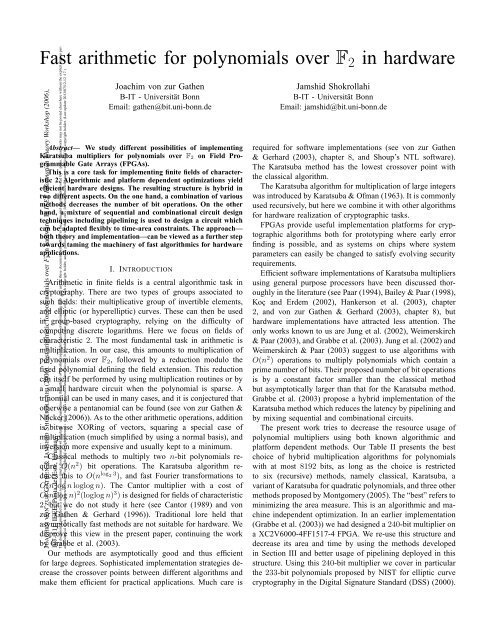
<strong>Fast</strong> <strong>ar<strong>it</strong>hmetic</strong> <strong>for</strong> <strong>polynomials</strong> <strong>over</strong> <strong>F2</strong> <strong>in</strong> <strong>hardware</strong><br />
JOACHIM VON ZUR GATHEN & JAMSHID SHOKROLLAHI (2006). <strong>Fast</strong> <strong>ar<strong>it</strong>hmetic</strong> <strong>for</strong> <strong>polynomials</strong> <strong>over</strong> <strong>F2</strong> <strong>in</strong> <strong>hardware</strong>. In IEEE In<strong>for</strong>mation Theory Workshop (2006),<br />
107–111. IEEE, Punta del Este, Uruguay.<br />
poses. These works may not be posted elsewhere w<strong>it</strong>hout the explic<strong>it</strong> wr<strong>it</strong>ten permission<br />
of the copyright holder. (Last update 2013/07/12-12 :17.)<br />
Joachim von zur Gathen<br />
B-IT - Univers<strong>it</strong>ät Bonn<br />
Email: gathen@b<strong>it</strong>.uni-bonn.de<br />
Abstract— We study different possibil<strong>it</strong>ies of implement<strong>in</strong>g<br />
Karatsuba multipliers <strong>for</strong> <strong>polynomials</strong> <strong>over</strong> <strong>F2</strong> on Field Programmable<br />
Gate Arrays (FPGAs).<br />
This is a core task <strong>for</strong> implement<strong>in</strong>g f<strong>in</strong><strong>it</strong>e fields of characteristic<br />
2. Algor<strong>it</strong>hmic and plat<strong>for</strong>m dependent optimizations yield<br />
efficient <strong>hardware</strong> designs. The result<strong>in</strong>g structure is hybrid <strong>in</strong><br />
two different aspects. On the one hand, a comb<strong>in</strong>ation of various<br />
methods decreases the number of b<strong>it</strong> operations. On the other<br />
hand, a mixture of sequential and comb<strong>in</strong>ational circu<strong>it</strong> design<br />
techniques <strong>in</strong>clud<strong>in</strong>g pipel<strong>in</strong><strong>in</strong>g is used to design a circu<strong>it</strong> which<br />
can be adapted flexibly to time-area constra<strong>in</strong>ts. The approach—<br />
both theory and implementation—can be viewed as a further step<br />
towards tam<strong>in</strong>g the mach<strong>in</strong>ery of fast algor<strong>it</strong>hmics <strong>for</strong> <strong>hardware</strong><br />
applications.<br />
<strong>in</strong>g any of these documents will adhere to the terms and constra<strong>in</strong>ts <strong>in</strong>voked by<br />
each copyright holder, and <strong>in</strong> particular use them only <strong>for</strong> noncommercial pur-<br />
I. INTRODUCTION<br />
Ar<strong>it</strong>hmetic <strong>in</strong> f<strong>in</strong><strong>it</strong>e fields is a central algor<strong>it</strong>hmic task <strong>in</strong><br />
cryptography. There are two types of groups associated to<br />
such fields: their multiplicative group of <strong>in</strong>vertible elements,<br />
and elliptic (or hyperelliptic) curves. These can then be used<br />
<strong>in</strong> group-based cryptography, rely<strong>in</strong>g on the difficulty of<br />
comput<strong>in</strong>g discrete logar<strong>it</strong>hms. Here we focus on fields of<br />
characteristic 2. The most fundamental task <strong>in</strong> <strong>ar<strong>it</strong>hmetic</strong> is<br />
multiplication. In our case, this amounts to multiplication of<br />
<strong>polynomials</strong> <strong>over</strong> <strong>F2</strong>, followed by a reduction modulo the<br />
fixed polynomial def<strong>in</strong><strong>in</strong>g the field extension. This reduction<br />
can <strong>it</strong>self be per<strong>for</strong>med by us<strong>in</strong>g multiplication rout<strong>in</strong>es or by<br />
a small <strong>hardware</strong> circu<strong>it</strong> when the polynomial is sparse. A<br />
tr<strong>in</strong>omial can be used <strong>in</strong> many cases, and <strong>it</strong> is conjectured that<br />
otherwise a pentanomial can be found (see von zur Gathen &<br />
Nöcker (2006)). As to the other <strong>ar<strong>it</strong>hmetic</strong> operations, add<strong>it</strong>ion<br />
is b<strong>it</strong>wise XOR<strong>in</strong>g of vectors, squar<strong>in</strong>g a special case of<br />
multiplication (much simplified by us<strong>in</strong>g a normal basis), and<br />
<strong>in</strong>version more expensive and usually kept to a m<strong>in</strong>imum.<br />
Classical methods to multiply two n-b<strong>it</strong> <strong>polynomials</strong> require<br />
O(n2 ) b<strong>it</strong> operations. The Karatsuba algor<strong>it</strong>hm reduces<br />
this to O(nlog2 3 ), and fast Fourier trans<strong>for</strong>mations to<br />
O(n log n loglog n). The Cantor multiplier w<strong>it</strong>h a cost of<br />
O(n(log n) 2 (loglog n) 3 ) is designed <strong>for</strong> fields of characteristic<br />
2, but we do not study <strong>it</strong> here (see Cantor (1989) and von<br />
zur Gathen & Gerhard (1996)). Trad<strong>it</strong>ional lore held that<br />
asymptotically fast methods are not su<strong>it</strong>able <strong>for</strong> <strong>hardware</strong>. We<br />
disprove this view <strong>in</strong> the present paper, cont<strong>in</strong>u<strong>in</strong>g the work<br />
by Grabbe et al. (2003).<br />
Our methods are asymptotically good and thus efficient<br />
<strong>for</strong> large degrees. Sophisticated implementation strategies decrease<br />
the cross<strong>over</strong> po<strong>in</strong>ts between different algor<strong>it</strong>hms and<br />
make them efficient <strong>for</strong> practical applications. Much care is<br />
are ma<strong>in</strong>ta<strong>in</strong>ed by the authors or by other copyright holders, notw<strong>it</strong>hstand<strong>in</strong>g that<br />
these works are posted here electronically. It is understood that all persons copy-<br />
This document is provided as a means to ensure timely dissem<strong>in</strong>ation of scholarly<br />
and technical work on a non-commercial basis. Copyright and all rights there<strong>in</strong><br />
Jamshid Shokrollahi<br />
B-IT - Univers<strong>it</strong>ät Bonn<br />
Email: jamshid@b<strong>it</strong>.uni-bonn.de<br />
required <strong>for</strong> software implementations (see von zur Gathen<br />
& Gerhard (2003), chapter 8, and Shoup’s NTL software).<br />
The Karatsuba method has the lowest cross<strong>over</strong> po<strong>in</strong>t w<strong>it</strong>h<br />
the classical algor<strong>it</strong>hm.<br />
The Karatsuba algor<strong>it</strong>hm <strong>for</strong> multiplication of large <strong>in</strong>tegers<br />
was <strong>in</strong>troduced by Karatsuba & Ofman (1963). It is commonly<br />
used recursively, but here we comb<strong>in</strong>e <strong>it</strong> w<strong>it</strong>h other algor<strong>it</strong>hms<br />
<strong>for</strong> <strong>hardware</strong> realization of cryptographic tasks.<br />
FPGAs provide useful implementation plat<strong>for</strong>ms <strong>for</strong> cryptographic<br />
algor<strong>it</strong>hms both <strong>for</strong> prototyp<strong>in</strong>g where early error<br />
f<strong>in</strong>d<strong>in</strong>g is possible, and as systems on chips where system<br />
parameters can easily be changed to satisfy evolv<strong>in</strong>g secur<strong>it</strong>y<br />
requirements.<br />
Efficient software implementations of Karatsuba multipliers<br />
us<strong>in</strong>g general purpose processors have been discussed thoroughly<br />
<strong>in</strong> the l<strong>it</strong>erature (see Paar (1994), Bailey & Paar (1998),<br />
Koç and Erdem (2002), Hankerson et al. (2003), chapter<br />
2, and von zur Gathen & Gerhard (2003), chapter 8), but<br />
<strong>hardware</strong> implementations have attracted less attention. The<br />
only works known to us are Jung et al. (2002), Weimerskirch<br />
& Paar (2003), and Grabbe et al. (2003). Jung et al. (2002) and<br />
Weimerskirch & Paar (2003) suggest to use algor<strong>it</strong>hms w<strong>it</strong>h<br />
O(n 2 ) operations to multiply <strong>polynomials</strong> which conta<strong>in</strong> a<br />
prime number of b<strong>it</strong>s. Their proposed number of b<strong>it</strong> operations<br />
is by a constant factor smaller than the classical method<br />
but asymptotically larger than that <strong>for</strong> the Karatsuba method.<br />
Grabbe et al. (2003) propose a hybrid implementation of the<br />
Karatsuba method which reduces the latency by pipel<strong>in</strong><strong>in</strong>g and<br />
by mix<strong>in</strong>g sequential and comb<strong>in</strong>ational circu<strong>it</strong>s.<br />
The present work tries to decrease the resource usage of<br />
polynomial multipliers us<strong>in</strong>g both known algor<strong>it</strong>hmic and<br />
plat<strong>for</strong>m dependent methods. Our Table II presents the best<br />
choice of hybrid multiplication algor<strong>it</strong>hms <strong>for</strong> <strong>polynomials</strong><br />
w<strong>it</strong>h at most 8192 b<strong>it</strong>s, as long as the choice is restricted<br />
to six (recursive) methods, namely classical, Karatsuba, a<br />
variant of Karatsuba <strong>for</strong> quadratic <strong>polynomials</strong>, and three other<br />
methods proposed by Montgomery (2005). The “best” refers to<br />
m<strong>in</strong>imiz<strong>in</strong>g the area measure. This is an algor<strong>it</strong>hmic and mach<strong>in</strong>e<br />
<strong>in</strong>dependent optimization. In an earlier implementation<br />
(Grabbe et al. (2003)) we had designed a 240-b<strong>it</strong> multiplier on<br />
a XC2V6000-4FF1517-4 FPGA. We re-use this structure and<br />
decrease <strong>it</strong>s area and time by us<strong>in</strong>g the methods developed<br />
<strong>in</strong> Section III and better usage of pipel<strong>in</strong><strong>in</strong>g deployed <strong>in</strong> this<br />
structure. Us<strong>in</strong>g this 240-b<strong>it</strong> multiplier we c<strong>over</strong> <strong>in</strong> particular<br />
the 233-b<strong>it</strong> <strong>polynomials</strong> proposed by NIST <strong>for</strong> elliptic curve<br />
cryptography <strong>in</strong> the Dig<strong>it</strong>al Signature Standard (DSS) (2000).
The structure of this paper is as follows. First the Karatsuba<br />
method and <strong>it</strong>s cost are studied <strong>in</strong> Section II. Section III is devoted<br />
to optimized hybrid Karatsuba implementations. Section<br />
IV shows how a hybrid structure and pipel<strong>in</strong><strong>in</strong>g together w<strong>it</strong>h<br />
the reduction of number of recursion levels improves resource<br />
usage <strong>in</strong> the circu<strong>it</strong> from Grabbe et al. (2003) and Section V<br />
concludes the paper.<br />
Parts of this paper have appeared <strong>in</strong> von zur Gathen &<br />
Shokrollahi (2005). The <strong>in</strong>clusion of Montgomery multiplication<br />
<strong>in</strong> Table II and the correspond<strong>in</strong>g considerations are<br />
presented here <strong>for</strong> the first time.<br />
II. THE KARATSUBA ALGORITHM<br />
The three coefficients of the product (a1x+a0)(b1x+b0) =<br />
a1b1x 2 + (a1b0 + a0b1)x + a0b0 are “classically” computed<br />
w<strong>it</strong>h 4 multiplications and 1 add<strong>it</strong>ion from the four <strong>in</strong>put<br />
coefficients a1, a0, b1, and b0. The follow<strong>in</strong>g <strong>for</strong>mula uses<br />
only 3 multiplications and 4 add<strong>it</strong>ions:<br />
(a1x + a0)(b1x + b0) = a1b1x 2 +<br />
((a1 + a0)(b1 + b0) − a1b1 − a0b0)x + a0b0. (1)<br />
We call this the 2-segment Karatsuba method or K2. Sett<strong>in</strong>g<br />
m = ⌈n/2⌉, two n-b<strong>it</strong> <strong>polynomials</strong> (thus of degrees less than<br />
n) can be rewr<strong>it</strong>ten and multiplied us<strong>in</strong>g the <strong>for</strong>mula:<br />
(f1x m + f0)(g1x m + g0) = h2x 2m + h1x m + h0,<br />
where f0, f1, g0, and g1 are m-b<strong>it</strong> <strong>polynomials</strong> respectively.<br />
The <strong>polynomials</strong> h0, h1, and h2 are computed by apply<strong>in</strong>g<br />
the Karatsuba algor<strong>it</strong>hm to the <strong>polynomials</strong> f0, f1, g0, and<br />
g1 as s<strong>in</strong>gle coefficients and add<strong>in</strong>g coefficients of common<br />
powers of x together. This method can be applied recursively.<br />
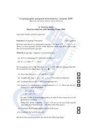
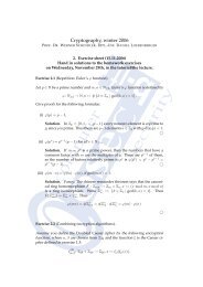
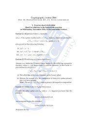
The circu<strong>it</strong> to per<strong>for</strong>m a s<strong>in</strong>gle stage is shown <strong>in</strong> Figure 1.<br />
f1 f0 g1 g0<br />
× + + ×<br />
−<br />
×<br />
+ −<br />
+<br />
<strong>over</strong>lap circu<strong>it</strong><br />
h2 h1 h0<br />
Fig. 1. One level of the Karatsuba multiplication<br />
The “<strong>over</strong>lap circu<strong>it</strong>” adds common powers of x <strong>in</strong> the three<br />
generated products. For example if n = 8, then the <strong>in</strong>put<br />
<strong>polynomials</strong> have degree at most 7, each of the <strong>polynomials</strong><br />
f0, f1, g0, and g1 is 4 b<strong>it</strong>s long and thus of degree at most<br />
3, and their products will be of degree at most 6. The effect<br />
of the <strong>over</strong>lap module <strong>in</strong> this case is represented <strong>in</strong> Figure 2,<br />
where coefficients to be added together are shown <strong>in</strong> the same<br />
columns.<br />
Figures 1 and 2 show that we need three multiplication calls<br />
at size m = ⌈n/2⌉ and some adders: 2 <strong>for</strong> <strong>in</strong>put, 2 <strong>for</strong> output,<br />
f1g1<br />
f0g1 + f1g0<br />
f0g0<br />
x 14 x 13 x 12 x 11 x 10 x 9 x 8<br />
x 10 x 9 x 8 x 7 x 6 x 5 x 4<br />
x 6 x 5 x 4 x 3 x 2 x 1 x 0<br />
Fig. 2. The <strong>over</strong>lap circu<strong>it</strong> <strong>for</strong> the 8-b<strong>it</strong> Karatsuba multiplier<br />
and 2 <strong>for</strong> the <strong>over</strong>lap module of lengths m, 2m − 1, and<br />
m − 1 respectively. Below we consider various algor<strong>it</strong>hms A<br />
of a similar structure. We denote the size reduction factor,<br />
the number of multiplications, <strong>in</strong>put adders, output adders,<br />
and the total number of b<strong>it</strong> operations to multiply two nb<strong>it</strong><br />
<strong>polynomials</strong> <strong>in</strong> A by bA, mulA, iaA, oaA, and MA(n),<br />
respectively. Then<br />
MA(n) = mulA M(m) + iaA m + oaA (2m − 1)+<br />
2(bA − 1)(m − 1),<br />
where m = ⌈n/bA⌉ and M(m) is the cost of the multiplication<br />
call <strong>for</strong> m-b<strong>it</strong> <strong>polynomials</strong>. For A = K2, this becomes:<br />
MK2(n) = 3 M(m) + 8m − 4, m = ⌈n/2⌉.<br />
Our <strong>in</strong>terest is not the usual recursive deployment of<br />
this k<strong>in</strong>d of algor<strong>it</strong>hms, but rather the efficient <strong>in</strong>teraction<br />
of various methods. We <strong>in</strong>clude <strong>in</strong> our study the classical<br />
multiplication Cb on b-b<strong>it</strong> <strong>polynomials</strong> and algor<strong>it</strong>hms <strong>for</strong> 3,<br />
5, 6, and 7-segment <strong>polynomials</strong> which we call K3 (3-segment<br />
Karatsuba, see Blahut (1985), Section 3.4, page 85), M5, M6,<br />
and M7 (see Montgomery (2005)). The parameters of these<br />
algor<strong>it</strong>hms are given <strong>in</strong> Table I.<br />
TABLE I<br />
THE PARAMETERS OF SOME MULTIPLICATION METHODS<br />
Algor<strong>it</strong>hm A bA mulA iaA oaA<br />
K2 2 3 2 2<br />
K3 3 6 6 6<br />
M5 5 13 22 30<br />
M6 6 17 61 40<br />
M7 7 22 21 55<br />
Cb, b ≥ 2 b b 2<br />
0 (b − 1) 2<br />
III. HYBRID DESIGN<br />
For fast multiplication software, a judicious mixture of table<br />
look-up and classical, Karatsuba and even faster (FFT) algor<strong>it</strong>hms<br />
must be used (see von zur Gathen & Gerhard (2003),<br />
chapter 8, and Hankerson et al. (2003), chapter 2). Su<strong>it</strong>able<br />
techniques <strong>for</strong> <strong>hardware</strong> implementations are not thoroughly<br />
studied <strong>in</strong> the l<strong>it</strong>erature. In contrast to software implementations<br />
where the word-length of the processor, the datapath, and<br />
the set of commands are fixed, <strong>hardware</strong> designers have more<br />
flexibil<strong>it</strong>y. In software solutions speed and memory usage are<br />
the measures of comparison whereas <strong>hardware</strong> implementations<br />
are generally designed to m<strong>in</strong>imize the area and time,<br />
simultaneously or w<strong>it</strong>h some weight-factors. In this section<br />
we determ<strong>in</strong>e the least-cost comb<strong>in</strong>ation of any basic rout<strong>in</strong>es<br />
<strong>for</strong> b<strong>it</strong> sizes up to 8192. Here, cost corresponds to the total<br />
number of operations <strong>in</strong> software, and the area <strong>in</strong> <strong>hardware</strong>.<br />
Us<strong>in</strong>g pipel<strong>in</strong><strong>in</strong>g and the structure of Grabbe et al. (2003)<br />
(2)
this can also result <strong>in</strong> multipliers which have small time-area<br />
parameters.<br />
We present a general methodology <strong>for</strong> this purpose. We<br />
start w<strong>it</strong>h a toolbox T of basic algor<strong>it</strong>hms, namely T =<br />
{classical, K2, K3, M5, M6, M7}. Each A ∈ T is def<strong>in</strong>ed <strong>for</strong><br />
bA-b<strong>it</strong> <strong>polynomials</strong>. We denote by T ∗ the set of all <strong>it</strong>erated<br />
(or hybrid algor<strong>it</strong>hms) compos<strong>it</strong>ions from T ; this <strong>in</strong>cludes T<br />
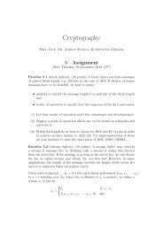
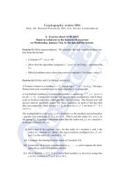
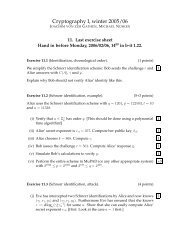
and the ident<strong>it</strong>y. Figure 3 shows the hierarchy of a hybrid<br />
algor<strong>it</strong>hm <strong>for</strong> 12-b<strong>it</strong> <strong>polynomials</strong> us<strong>in</strong>g our toolbox T . At<br />
the top level, K2 is used, mean<strong>in</strong>g that the 12-b<strong>it</strong> <strong>in</strong>put<br />
<strong>polynomials</strong> are divided <strong>in</strong>to two 6-b<strong>it</strong> <strong>polynomials</strong> each and<br />
K2 is used to multiply the <strong>in</strong>put <strong>polynomials</strong> as if each 6-b<strong>it</strong><br />
polynomial were a s<strong>in</strong>gle coefficient. K2C3 per<strong>for</strong>ms the three<br />
6-b<strong>it</strong> multiplications. One of these 6-b<strong>it</strong> multipliers is circled<br />
<strong>in</strong> Figure 3 and unravels as follows:<br />
(a5x 5 + · · · + a0) · (b5x 5 + · · · + b0) =<br />
((a5x 2 + a4x + a3)x 3 + (a2x 2 + a1x + a0))<br />
· ((b5x 2 + b4x + b3)x 3 + (b2x 2 + b1x + b0)) =<br />
(A1x 3 + A0) · (B1x 3 + B0) = A1B1x 6 +<br />
((A1 + A0)(B1 + B0) − A1B1 − A0B0)x 3 + A0B0<br />
Each of A1B1, (A1 + A0)(B1 + B0), and A0B0 denotes a<br />
multiplication of 3-b<strong>it</strong> <strong>polynomials</strong> and will be done classically<br />
us<strong>in</strong>g the <strong>for</strong>mula<br />
(a2x 2 + a1x + a0)(b2x 2 + b1x + b0) = a2b2x 4 +<br />
(a2b1 + a1b2)x 3 + (a2b0 + a1b1 + a0b2)x 2 +<br />
(a1b0 + a0b1)x + a0b0.<br />
Thick l<strong>in</strong>es under each C3 <strong>in</strong>dicate the n<strong>in</strong>e 1-b<strong>it</strong> multiplications<br />
to per<strong>for</strong>m C3. We designate this algor<strong>it</strong>hm, <strong>for</strong> 12b<strong>it</strong><br />
<strong>polynomials</strong>, w<strong>it</strong>h K2K2C3 = K 2 2 C3 where the left hand<br />
algor<strong>it</strong>hm, <strong>in</strong> this case K2, is the topmost algor<strong>it</strong>hm.<br />
K2<br />
K2 K2 K2<br />
C3 C3 C3 C3 C3 C3 C3 C3 C3<br />
Fig. 3. The multiplication hierarchy <strong>for</strong> K2K2C3<br />
As <strong>in</strong> (2), the cost of a hybrid algor<strong>it</strong>hm A2A1 ∈ T ∗ w<strong>it</strong>h<br />
A1, A2 ∈ T ∗ satisfies<br />
MA2A1(n) ≤mulA2 MA1(m) + iaA2 m+<br />
oaA2 (2m − 1) + 2(bA2 − 1)(m − 1), (3)<br />
where MA(1) = 1 <strong>for</strong> any A ∈ T ∗ and m = ⌈n/(bA2bA1)⌉ =<br />
⌈⌈n/bA2⌉/bA1⌉. Each A ∈ T ∗ has a well-def<strong>in</strong>ed <strong>in</strong>put length<br />
bA, given <strong>in</strong> Table I <strong>for</strong> basic tools and by multiplication <strong>for</strong><br />
compos<strong>it</strong>e methods. We extend the notion by apply<strong>in</strong>g A also<br />
to fewer than bA b<strong>it</strong>s, by padd<strong>in</strong>g w<strong>it</strong>h lead<strong>in</strong>g zeros, so that<br />
MA(m) = MA(bA) <strong>for</strong> 1 ≤ m ≤ bA. For some purposes,<br />
one might consider the sav<strong>in</strong>gs due to such a-priori-zero<br />
coefficients. Our goal, however, is a pipel<strong>in</strong>ed structure where<br />
such a consideration cannot be <strong>in</strong>corporated. The m<strong>in</strong>imum<br />
hybrid cost <strong>over</strong> T is<br />
M(n) = m<strong>in</strong><br />
A∈T ∗ ,bA≥n MA(n).<br />
We first show that the <strong>in</strong>f<strong>in</strong><strong>it</strong>ely many classical algor<strong>it</strong>hms<br />
<strong>in</strong> T do not contribute to optimal methods beyond size 12.<br />
Lemma 1: For A ∈ T ∗ and <strong>in</strong>tegers m ≥ 1 and b, c ≥ 2 we<br />
have the follow<strong>in</strong>g.<br />
(i) MCbCc(bc) = MCbc (bc).<br />
(ii) MCbA(bAbm) ≥ MACb (bAbm).<br />
(iii) For any n, there is an optimal hybrid algor<strong>it</strong>hm all of<br />
whose components are non-classical, except possibly the<br />
right most one.<br />
(iv) If n ≥ 13, then Cn is not optimal.<br />
We now present a dynamic programm<strong>in</strong>g algor<strong>it</strong>hm which<br />
computes an optimal hybrid algor<strong>it</strong>hm from T ∗ <strong>for</strong> n-b<strong>it</strong><br />
multiplication, <strong>for</strong> n = 1, 2, . . ..<br />
Algor<strong>it</strong>hm 1 F<strong>in</strong>d<strong>in</strong>g optimal algor<strong>it</strong>hms <strong>in</strong> T ∗<br />
Input: The toolbox T = {classical, K2, K3, M5, M6, M7}<br />
and an <strong>in</strong>teger N.<br />
Output: Table T w<strong>it</strong>h N rows conta<strong>in</strong><strong>in</strong>g the optimal algor<strong>it</strong>hms<br />
<strong>for</strong> 1 ≤ n ≤ N and their costs.<br />
1: Enter the classical algor<strong>it</strong>hm and cost 1 <strong>for</strong> n = 1 <strong>in</strong>to T<br />
2: <strong>for</strong> n = 2, . . . , N do<br />
3: bestalgor<strong>it</strong>hm ← unknown, m<strong>in</strong>cost ← +<strong>in</strong>f<strong>in</strong><strong>it</strong>y<br />
4: <strong>for</strong> A = K2, . . . , M7 do<br />
5: Compute MA(n) accord<strong>in</strong>g to (2)<br />
6: if MA(n) < m<strong>in</strong>cost then<br />
7: bestalgor<strong>it</strong>hm ← A, m<strong>in</strong>cost ← MA(n)<br />
8: end if<br />
9: end <strong>for</strong><br />
10: if n < 13 then<br />
11: MCn ← 2n 2 − 2n + 1<br />
12: if MCn(n) < m<strong>in</strong>cost then<br />
13: bestalgor<strong>it</strong>hm ← Cn, m<strong>in</strong>cost ← MCn(n)<br />
14: end if<br />
15: end if<br />
16: Enter bestalgor<strong>it</strong>hm and m<strong>in</strong>cost <strong>for</strong> n <strong>in</strong>to T<br />
17: end <strong>for</strong><br />
Theorem 2: Algor<strong>it</strong>hm 1 works correctly as specified. The<br />
operations (<strong>ar<strong>it</strong>hmetic</strong>, table look-up) have <strong>in</strong>tegers w<strong>it</strong>h<br />
O(log N) b<strong>it</strong>s as <strong>in</strong>put, and their total number is O(N).<br />
The optimal recursive method <strong>for</strong> each polynomial length up<br />
to 8192 is shown <strong>in</strong> Table II. The column “length” of this table<br />
represents the length (or the range of lengths) of <strong>polynomials</strong><br />
<strong>for</strong> which the method specified <strong>in</strong> the column “method” must<br />
be used. As an example, <strong>for</strong> 194-b<strong>it</strong> <strong>polynomials</strong> the method<br />
M7 is used at the top level. This requires 22 multiplications<br />
of <strong>polynomials</strong> w<strong>it</strong>h ⌈194/7⌉ = 28 b<strong>it</strong>s, which are done<br />
by means of K2 on top of 14-b<strong>it</strong> <strong>polynomials</strong>. These 14b<strong>it</strong><br />
multiplications are executed aga<strong>in</strong> us<strong>in</strong>g K2 and f<strong>in</strong>ally<br />
<strong>polynomials</strong> of length 7 are multiplied classically. Thus the
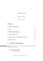
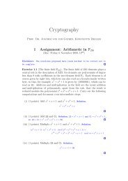
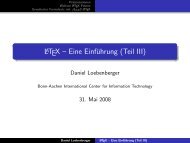
Number of b<strong>it</strong> operations × 10 −3<br />
10<br />
5<br />
classical<br />
Karatsuba<br />
hybrid<br />
32 64 96 128<br />
Polynomial length<br />
Fig. 4. The number of b<strong>it</strong> operations of the classical, recursive Karatsuba,<br />
and the hybrid methods to multiply <strong>polynomials</strong> of degree smaller than 128<br />
TABLE II<br />
OPTIMAL MULTIPLICATIONS FOR POLYNOMIAL LENGTHS UP TO 8192<br />
length method length method length method<br />
1 − 5 C 1 − C 5 301 − 320 K 2 1603 − 1610 M 5<br />
6 K 2 321 − 343 M 7 1611 − 1728 M 6<br />
7 C 7 344 − 360 M 5 1729 − 1792 M 7<br />
8 K 2 361 − 384 K 2 1793 − 1800 M 5<br />
9 K 3 385 − 392 M 7 1801 − 1920 M 6<br />
10 K 2 393 − 400 M 5 1921 − 1960 M 7<br />
11 C 11 401 − 420 M 7 1961 − 2048 K 2<br />
12 − 14 K 2 421 − 432 K 2 2049 − 2058 M 7<br />
15 K 3 433 − 448 M 7 2059 − 2100 M 5<br />
16 − 20 K 2 449 − 450 M 5 2101 − 2240 M 7<br />
21 M 7 451 − 454 K 2 2241 − 2304 M 6<br />
22 − 24 K 2 455 M 5 2305 − 2352 M 7<br />
25 M 5 456 K 2 2353 − 2400 M 6<br />
26 − 27 K 3 457 − 460 M 5 2401 − 2560 K 2<br />
28 − 40 K 2 461 − 512 K 2 2561 − 2744 M 7<br />
41 − 42 M 7 513 − 525 M 5 2745 − 2800 M 5<br />
43 − 45 K 3 526 − 560 M 7 2801 − 2880 M 6<br />
46 − 48 K 2 561 − 576 K 2 2881 − 3072 K 2<br />
49 M 7 577 − 588 M 7 3073 − 3136 M 7<br />
50 M 5 589 − 600 M 5 3137 − 3200 M 5<br />
51 − 64 K 2 601 − 640 K 2 3201 − 3456 M 6<br />
65 − 70 M 7 641 − 686 M 7 3457 − 3584 M 7<br />
71 − 80 K 2 687 − 720 M 5 3585 − 3840 M 6<br />
81 − 84 M 7 721 − 768 K 2 3841 − 3920 M 7<br />
85 − 96 K 2 769 − 784 M 7 3921 − 4096 K 2<br />
97 − 98 M 7 785 − 800 M 5 4097 − 4116 M 7<br />
99 − 100 M 5 801 − 840 M 7 4117 − 4200 M 5<br />
101 − 105 M 7 841 − 864 M 6 4201 − 4320 M 6<br />
106 − 108 K 2 865 − 896 M 7 4321 − 4480 M 7<br />
109 − 112 M 7 897 − 900 M 5 4481 − 4608 M 6<br />
113 − 128 K 2 901 − 912 M 6 4609 − 4704 M 7<br />
129 − 140 M 7 913 − 920 M 5 4705 − 4800 M 6<br />
141 − 144 K 2 921 − 936 M 6 4801 − 5120 K 2<br />
145 − 147 M 7 937 − 940 M 5 5121 − 5184 M 6<br />
148 − 150 M 5 941 − 960 M 6 5185 − 5488 M 7<br />
151 − 160 K 2 961 − 980 M 7 5489 − 5600 M 5<br />
161 − 168 M 7 981 − 1024 K 2 5601 − 5880 M 6<br />
169 − 175 M 5 1025 − 1029 M 7 5881 − 5888 K 2<br />
176 − 192 K 2 1030 − 1050 M 5 5889 − 5952 M 6<br />
193 − 196 M 7 1051 − 1120 M 7 5953 − 6016 K 2<br />
197 − 200 M 5 1121 − 1152 M 6 6017 − 6144 M 6<br />
201 − 210 M 7 1153 − 1176 M 7 6145 − 6272 M 7<br />
211 − 216 K 2 1177 − 1200 M 5 6273 − 6400 M 5<br />
217 − 224 M 7 1201 − 1280 K 2 6401 − 6912 M 6<br />
225 M 5 1281 − 1372 M 7 6913 − 7168 M 7<br />
226 − 256 K 2 1373 − 1440 M 5 7169 − 7680 M 6<br />
257 − 280 M 7 1441 − 1536 K 2 7681 − 7840 M 7<br />
281 − 288 K 2 1537 − 1568 M 7 7841 − 8064 M 6<br />
289 − 294 M 7 1569 − 1600 M 5 8065 − 8192 K 2<br />
295 − 300 M 5 1601 − 1602 M 6<br />
optimal algor<strong>it</strong>hm is A = M7K2 2C7, of total cost MA(194) =<br />
22 · MK2 2C7 (28) + 3937 = 26575 b<strong>it</strong> operations.<br />
Figure 4 shows the recursive cost of the Karatsuba method,<br />
as used <strong>in</strong> Weimerskirch & Paar (2003), of our hybrid method,<br />
and the classical method.<br />
Lemma 1 implies that the classical methods need only be<br />
considered <strong>for</strong> n ≤ 12. We can prune T further and now<br />
illustrate this <strong>for</strong> K3. One first checks that MAK3B(3bAbB) <<br />
MK3AB(3bAbB) <strong>for</strong> A ∈ {K2, M5, M6, M7}, B ∈ T ∗ , and<br />
bB ≥ 2. There<strong>for</strong>e <strong>for</strong> K3 to be the top-level tool <strong>in</strong> an optimal<br />
algor<strong>it</strong>hm <strong>over</strong> T the next algor<strong>it</strong>hm to <strong>it</strong> must be e<strong>it</strong>her K3<br />
or Cb <strong>for</strong> some b. S<strong>in</strong>ce the classical method is not optimal<br />
<strong>for</strong> n ≥ 13 and Table II does not list K3 <strong>in</strong> the <strong>in</strong>terval 46 to<br />
3 · 45 = 135, K3 is not the top-level tool <strong>for</strong> n ≥ 135.<br />
Table III gives the asymptotic behavior of the costs of the<br />
algor<strong>it</strong>hms <strong>in</strong> the toolbox T when used recursively. It is expected<br />
that <strong>for</strong> very large <strong>polynomials</strong> only the asymptotically<br />
fastest method, namely M6, should be used. But due to the t<strong>in</strong>y<br />
differences <strong>in</strong> the cost exponents this seems to happen only<br />
<strong>for</strong> very large polynomial lengths, beyond the sizes which are<br />
shown <strong>in</strong> Table II.<br />
TABLE III<br />
ASYMPTOTICAL COST O(n k ) OF ALGORITHMS IN THE TOOLBOX T<br />
algor<strong>it</strong>hm k<br />
Cb, b ≥ 2 logb b 2 = 2<br />
K2 log2 3 ≈ 1.5850<br />
K3 log3 6 ≈ 1.6309<br />
M5 log5 13 ≈ 1.5937<br />
M6 log6 17 ≈ 1.5812<br />
M7 log7 22 ≈ 1.5885<br />
IV. HARDWARE STRUCTURE<br />
The delay of a fully parallel comb<strong>in</strong>ational Karatsuba multiplier<br />
is 4⌈log 2 n⌉, which is almost 4 times that of a classical<br />
multiplier, namely ⌈log 2 n⌉+1. It is the ma<strong>in</strong> disadvantage of<br />
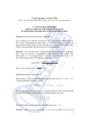
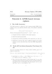
the Karatsuba method <strong>for</strong> <strong>hardware</strong> implementations. Grabbe<br />
et al. (2003) suggested as solution a pipel<strong>in</strong>ed Karatsuba<br />
multiplier <strong>for</strong> 240-b<strong>it</strong> <strong>polynomials</strong>, shown <strong>in</strong> Figure 5.<br />
240-b<strong>it</strong> multiplier<br />
120-b<strong>it</strong> multiplier<br />
40-b<strong>it</strong><br />
multiplier<br />
Overlap module<br />
40-b<strong>it</strong> adder<br />
· · ·<br />
79-b<strong>it</strong> adder<br />
· · ·<br />
Overlap module<br />
120-b<strong>it</strong> adder<br />
· · ·<br />
239-b<strong>it</strong> adder<br />
· · ·<br />
Fig. 5. The 240-b<strong>it</strong> multiplier by Grabbe et al. (2003)<br />
The <strong>in</strong>nermost part of the design is a comb<strong>in</strong>ational<br />
pipel<strong>in</strong>ed 40-b<strong>it</strong> classical multiplier equipped w<strong>it</strong>h 40-b<strong>it</strong> and<br />
79-b<strong>it</strong> adders. The multiplier, these adders, and the <strong>over</strong>lap<br />
module, together w<strong>it</strong>h a control circu<strong>it</strong>, const<strong>it</strong>ute a 120-b<strong>it</strong><br />
multiplier. The algor<strong>it</strong>hm is based on a modification of a<br />
Karatsuba <strong>for</strong>mula <strong>for</strong> 3-segment <strong>polynomials</strong>. Another su<strong>it</strong>able<br />
control circu<strong>it</strong> per<strong>for</strong>ms the 2-segment Karatsuba method<br />
<strong>for</strong> 240 b<strong>it</strong>s by means of a 120-b<strong>it</strong> recursion, 239-b<strong>it</strong> adders,<br />
and an <strong>over</strong>lap circu<strong>it</strong>.<br />
We improve this multiplier w<strong>it</strong>h respect to both area and<br />
time. The multiplier of Grabbe et al. (2003) can be seen as<br />
implement<strong>in</strong>g the factorization 240 = 2·3·40. Table III implies<br />
that <strong>it</strong> is usually best to apply the 3-segment Karatsuba <strong>for</strong><br />
small <strong>in</strong>puts. Translat<strong>in</strong>g this <strong>in</strong>to <strong>hardware</strong> real<strong>it</strong>y, the new<br />
design is based on the factorization 240 = 2 · 2 · 2 · 30.<br />
The new 30-b<strong>it</strong> multiplier follows the recipe of Table II.<br />
It is a comb<strong>in</strong>ational circu<strong>it</strong> w<strong>it</strong>hout feedback and the design<br />
goal is to m<strong>in</strong>imize <strong>it</strong>s area. In general, k pipel<strong>in</strong>e stages can
control module<br />
<strong>in</strong>put1 <strong>in</strong>put2<br />
a(x) b(x)<br />
mux1 mux2<br />
mux3 mux4<br />
mux5 mux6<br />
30 b<strong>it</strong><br />
multiplier<br />
decoder<br />
acc0 acc1 · · · acc14<br />
<strong>over</strong>lap circu<strong>it</strong><br />
output<br />
Fig. 6. The structure of the Karatsuba multiplier w<strong>it</strong>h few recursions<br />
per<strong>for</strong>m n parallel multiplications <strong>in</strong> n + k − 1 <strong>in</strong>stead of nk<br />
clock cycles w<strong>it</strong>hout pipel<strong>in</strong><strong>in</strong>g.<br />
In the recursive Karatsuba multiplier of Grabbe et al. (2003),<br />
the core of the system, namely the comb<strong>in</strong>ational multiplier,<br />
is idle <strong>for</strong> about half of the time. To improve the resource<br />
usage, we reduce the communication <strong>over</strong>head by decreas<strong>in</strong>g<br />
the levels of recursion. In this new 240-b<strong>it</strong> multiplier, an 8segment<br />
Karatsuba is applied at once to 30-b<strong>it</strong> <strong>polynomials</strong>.<br />
We computed symbolically the <strong>for</strong>mulas describ<strong>in</strong>g three<br />
recursive levels of Karatsuba, and implemented these <strong>for</strong>mulas<br />
directly.<br />
The new circu<strong>it</strong> is shown <strong>in</strong> Figure 6. The multiplexers mux1<br />
to mux6 are adders at the same time. Their <strong>in</strong>puts are 30-b<strong>it</strong><br />
sections of the two orig<strong>in</strong>al 240-b<strong>it</strong> <strong>polynomials</strong> which are<br />
added accord<strong>in</strong>g to the Karatsuba rules. Now their 27 output<br />
pairs are pipel<strong>in</strong>ed as <strong>in</strong>puts <strong>in</strong>to the 30-b<strong>it</strong> multiplier. The 27<br />
correspond<strong>in</strong>g 59-b<strong>it</strong> <strong>polynomials</strong> are subsequently comb<strong>in</strong>ed<br />
accord<strong>in</strong>g to the <strong>over</strong>lap rules to yield the f<strong>in</strong>al result. The<br />
synchronization is set so that the 30-b<strong>it</strong> multipliers require<br />
1 and 4 clock cycles <strong>for</strong> the classical and hybrid Karatsuba<br />
implementations, respectively.<br />
The time and space consumptions after place and route<br />
are shown <strong>in</strong> Table IV and compared w<strong>it</strong>h the results of<br />
Grabbe et al. (2003) and the classical method. The second<br />
column shows the number of clock cycles <strong>for</strong> a multiplication.<br />
The third column represents the area <strong>in</strong> terms of number of<br />
slices. This measure conta<strong>in</strong>s both logic elements, or LUTs,<br />
and flip-flops used <strong>for</strong> pipel<strong>in</strong><strong>in</strong>g. The fourth column is the<br />
multiplication time as returned by the <strong>hardware</strong> synthesis tool.<br />
F<strong>in</strong>ally the last column shows the product of area and time <strong>in</strong><br />
order to compare the AT measures of our designs.<br />
V. CONCLUSION<br />
In this paper we have shown how comb<strong>in</strong><strong>in</strong>g algor<strong>it</strong>hmic<br />
techniques w<strong>it</strong>h plat<strong>for</strong>m dependent strategies can be used to<br />
develop designs which are highly optimized <strong>for</strong> FPGAs. These<br />
modules have been considered as appropriate implementation<br />
TABLE IV<br />
TIME AND AREA OF DIFFERENT 240-BIT MULTIPLIERS<br />
multiplier clock slices time AT<br />
type cycles Slices × µs<br />
classical 56 1582 0.523µs 827<br />
the circu<strong>it</strong> of Fig. 5 54 1660 0.655µs 1087<br />
hybrid (Fig. 6) 30 1480 0.378µs 559<br />
targets <strong>for</strong> cryptographic purposes both as prototyp<strong>in</strong>g plat<strong>for</strong>ms<br />
and as system on chips.<br />
The benef<strong>it</strong>s of hybrid implementations are well known <strong>for</strong><br />
software implementations, where the cross<strong>over</strong> po<strong>in</strong>ts between<br />
subquadratic and classical methods depend on the available<br />
memory and processor word size. There seems to be no previous<br />
systematic <strong>in</strong>vestigation on how to apply these methods<br />
efficiently <strong>for</strong> <strong>hardware</strong> implementations. We have shown that<br />
a hybrid implementation mix<strong>in</strong>g classical and asymptotically<br />
fast recursive methods can result <strong>in</strong> significant area sav<strong>in</strong>gs.<br />
REFERENCES<br />
[1] D. V. Bailey and C. Paar, “Optimal extension fields <strong>for</strong> fast <strong>ar<strong>it</strong>hmetic</strong><br />
<strong>in</strong> public-key algor<strong>it</strong>hms,” <strong>in</strong> Advances <strong>in</strong> Cryptology: Proceed<strong>in</strong>gs<br />
of CRYPTO ’98, Santa Barbara CA, ser. Lecture Notes <strong>in</strong> Computer<br />
Science, H. Krawczyk, Ed., no. 1462. Spr<strong>in</strong>ger-Verlag, 1998, pp. 472–<br />
485.<br />
[2] R. E. Blahut, <strong>Fast</strong> Algor<strong>it</strong>hms <strong>for</strong> Dig<strong>it</strong>al Signal Process<strong>in</strong>g. Read<strong>in</strong>g<br />
MA: Addison-Wesley, 1985.<br />
[3] D. G. Cantor, “On <strong>ar<strong>it</strong>hmetic</strong>al algor<strong>it</strong>hms <strong>over</strong> f<strong>in</strong><strong>it</strong>e fields,” Journal of<br />
Comb<strong>in</strong>atorial Theory, Series A, vol. 50, pp. 285–300, 1989.<br />
[4] Dig<strong>it</strong>al Signature Standard (DSS), U.S. Department of Commerce /<br />
National Inst<strong>it</strong>ute of Standards and Technology, January 2000, federal<br />
In<strong>for</strong>mation Process<strong>in</strong>gs Standards Publication 186-2.<br />
[5] J. von zur Gathen and J. Gerhard, “Ar<strong>it</strong>hmetic and factorization of<br />
<strong>polynomials</strong> <strong>over</strong> <strong>F2</strong>,” <strong>in</strong> Proceed<strong>in</strong>gs of the 1996 International Symposium<br />
on Symbolic and Algebraic Computation ISSAC ’96, Zürich,<br />
Sw<strong>it</strong>zerland, Y. N. Lakshman, Ed. ACM Press, 1996, pp. 1–9.<br />
[6] ——, Modern Computer Algebra, 2nd ed. Cambridge, UK: Cambridge<br />
Univers<strong>it</strong>y Press, 2003, first ed<strong>it</strong>ion 1999.<br />
[7] J. von zur Gathen and M. Nöcker, “Polynomial and normal bases<br />
<strong>for</strong> f<strong>in</strong><strong>it</strong>e fields,” Journal of Cryptology, vol. 18, no. 4, pp. 337–355,<br />
September 2005.<br />
[8] J. von zur Gathen and J. Shokrollahi, “Efficient FPGA-based Karatsuba<br />
multipliers <strong>for</strong> <strong>polynomials</strong> <strong>over</strong> <strong>F2</strong>,” <strong>in</strong> Selected Areas <strong>in</strong> Cryptography<br />
(SAC 2005). Spr<strong>in</strong>ger-Verlag, 2005, to appear.<br />
[9] C. Grabbe, M. Bednara, J. Shokrollahi, J. Teich, and J. von zur Gathen,<br />
“FPGA designs of parallel high per<strong>for</strong>mance GF(2 233 ) multipliers,”<br />
<strong>in</strong> Proc. of the IEEE International Symposium on Circu<strong>it</strong>s and Systems<br />
(ISCAS-03), vol. II, Bangkok, Thailand, May 2003, pp. 268–271.<br />
[10] D. Hankerson, A. Menezes, and S. Vanstone, Guide to Elliptic Curve<br />
Cryptography. Spr<strong>in</strong>ger-Verlag, 2003.<br />
[11] M. Jung, F. Madlener, M. Ernst, and S. Huss, “A Reconfigurable<br />
Coprocessor <strong>for</strong> F<strong>in</strong><strong>it</strong>e Field Multiplication <strong>in</strong> GF(2 n ),” <strong>in</strong> Workshop<br />
on Cryptographic Hardware and Embedded Systems. Hamburg: IEEE,<br />
April 2002.<br />
[12] A. Karatsuba and Y. Ofman, “Multiplication of multidig<strong>it</strong> numbers on<br />
automata,” Soviet Physics–Doklady, vol. 7, no. 7, pp. 595–596, January<br />
1963, translated from Doklady Akademii Nauk SSSR, Vol. 145, No. 2,<br />
pp. 293–294, July, 1962.<br />
[13] Ç. K. Koç and S. S. Erdem, “Improved Karatsuba-Ofman Multiplication<br />
<strong>in</strong> GF(2 m ),” US Patent Application, January 2002.<br />
[14] P. L. Montgomery, “Five, Six, and seven-Term Karatsuba-Like Formulae,”<br />
IEEE Transactions on Computers, vol. 54, no. 3, pp. 362–369,<br />
March 2005.<br />
[15] C. Paar, “Efficient VLSI Arch<strong>it</strong>ectures <strong>for</strong> B<strong>it</strong>-Parallel Computation <strong>in</strong><br />
Galois Fields,” Ph.D. dissertation, Inst<strong>it</strong>ute <strong>for</strong> Experimental Mathematics,<br />
Univers<strong>it</strong>y of Essen, Essen, Germany, June 1994.<br />
[16] A. Weimerskirch and C. Paar, “Generalizations of the Karatsuba Algor<strong>it</strong>hm<br />
<strong>for</strong> Efficient Implementations,” Ruhr-Univers<strong>it</strong>ät-Bochum, Germany,<br />
Tech. Rep., 2003.