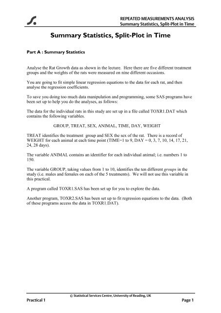
Summary Statistics, Split-Plot in Time - University of Reading

REPEATED MEASUREMENTS ANALYSIS
Summary Statistics, Split-Plot in Time
Summary Statistics, Split-Plot in Time
Part A : Summary Statistics
Analyse the Rat Growth data as shown in the lecture. Here there are five different treatment
groups and the weights of the rats were measured on nine different occasions.
You are going to fit simple linear regression equations to the data for each rat, and then
analyse the regression coefficients.
To save you doing too much data manipulation and programming, some SAS programs have
been set up to help you do the analyses, as follows:
The data for the individual rats in this study are set up in a file called TOXR1.DAT which
contains the following variables.
GROUP, TREAT, SEX, ANIMAL, TIME, DAY, WEIGHT
TREAT identifies the treatment group and SEX the sex of the rat. There is a record of
WEIGHT for each animal at each time point (TIME=1 to 9, DAY = 0, 3, 7, 10, 14, 17, 21,
24, 28 days).
The variable ANIMAL contains an identifier for each individual animal; i.e. numbers 1 to
150.
The variable GROUP, taking values from 1 to 10, identifies the ten different groups in the
study (i.e. males and females on each of the 5 treatments). We will not use this variable in
this practical.
A program called TOXR1.SAS has been set up for you to explore the data.
Another program, TOXR2.SAS has been set up to fit regression equations to the data. (Both
of these programs access the data in TOXR1.DAT).
© Statistical Services Centre, University of Reading, UK
Practical 1 Page 1

REPEATED MEASUREMENTS ANALYSIS
Summary Statistics, Split-Plot in Time
(i) First of all, using TOXR1.SAS, look at the profiles for the individual rats.
The code to do this is all set up for you in the program. All you have to do is run it.
Do you see any consistent pattern to the individual rat profiles?
Do the profiles seem linear?
(ii) Now, using TOXR2.SAS, try fitting the following simple curve to the profiles:
y = a + bt
where y is weight and t is day; and analyse the coefficient b.
Within the program TOXR2.SAS the curve is fitted for each rat using PROC REG,
and the coefficients are saved into temporary datasets called BETA and then
TOX_REG. Make sure you understand what the SAS commands are doing here.
Please ask if you are unsure.
Then use the dataset TOX_REG to analyse the coefficients. Look first of all at effects
due to sex, treatment and the sex*treatment interaction, e.g.
PROC GLM DATA = TOX_REG;
CLASS SEX TREAT;
MODEL DAY = SEX TREAT SEX*TREAT/SS2;
LSMEANS SEX TREAT SEX*TREAT;
RUN;
(iii) The five treatments in this experiment (numbered 1 to 5) were respectively: control,
compound A at 4, 20 and 100mg/kg/day and compound B at 100mg/kg/day. The
overall treatment effect can be broken down into treatment contrasts. Four contrasts
have been set up within the program for you to use. Make sure you are clear which
comparisons they relate to. Now analyse the data again, incorporating these contrasts.
What do you conclude?
© Statistical Services Centre, University of Reading, UK
Practical 1 Page 2

Part B : Split-Plot in Time
Question 1
REPEATED MEASUREMENTS ANALYSIS
Summary Statistics, Split-Plot in Time
Cardiac Enzyme Data. This is the experiment looking at the effects of preserving liquids on
the enzyme content of dog hearts. The ATP levels for the 23 dog hearts, recorded during a 12
hour period may be found in the file CARDENZ1.DAT. This file contains the following
variables:
HEART, A, B, ATP_0, ATP_1, ATP_2 to ATP_9
The two variables A and B are factors each at two levels, and it is the combination of these
two which constitutes the four preserving liquids which were studied in the experiment.
ATP_0 contains the baseline ATP value whilst ATP_1 to ATP_9 contain the values
following initial preservation.
A program called CARDENZ1.SAS has been set up for you to read in and analyse these data.
Using CARDENZ1.SAS carry out a split-plot-in-time analysis of variance on these data.
You will need PROC GLM with the REPEATED statement, as follows.
PROC GLM;
CLASS A B;
MODEL ATP_1-ATP_9 = A B A*B/SS2;
REPEATED TIME 9;
RUN;
The above will give you a separate analysis of variance for the data at each time point, as
well as the split plot in time analysis. Record below the residual mean squares from the
analyses of each time point.
ATP_1
ATP_2
ATP_3
ATP_4
ATP_5
ATP_6
ATP_7
ATP_8
ATP_9
Residual Mean Square
Does the variance appear to be constant across time?
Try out some of the different options which are available on the MODEL and REPEATED
statements.
© Statistical Services Centre, University of Reading, UK
Practical 1 Page 3

e.g. on the MODEL statement
REPEATED MEASUREMENTS ANALYSIS
Summary Statistics, Split-Plot in Time
/NOUNI will suppress all the analyses at the individual time points
on the REPEATED statement
/NOM will suppress any multivariate analyses
/PRINTE will give the partial correlation coefficients for the individual time
points, and sphericity tests. The sphericity test for the orthogonal components is the
test for the type H structure.
What do the results of the analysis show you?
What are the Greenhouse-Geisser and Huynh-Feldt estimates of ε( εɵ ~
ε)
and ?
And how is the significance of the interactions with time modified by using these two
adjustments to the degrees of freedom in the F-test.
What was the result of the Chi-square test for the type H structure? And how do you interpret
it?
Make sure your output agrees with the results in the lecture.
© Statistical Services Centre, University of Reading, UK
Practical 1 Page 4

Question 2
REPEATED MEASUREMENTS ANALYSIS
Summary Statistics, Split-Plot in Time
Carry out a split-plot-in-time anova using the Rat Growth data. You will now use the dataset
called TOXR2.DAT, which contains the variables TREAT, SEX, ANIMAL and Y0 to Y8,
where Y0 to Y8 contain the weights recorded at the nine times.
A program called TOXR3.SAS which accesses TOXR2.DAT has been set up for you to use
for this analysis.
(i) Investigate the data on rat weights, initially using the factors sex and group (and their
interaction). Again you will need to use PROC GLM with a REPEATED statement.
From the univariate analyses of the data at each time point, does it appear that the
variance of rat weight is constant over time? And what can you conclude from the
correlation matrix of the weights at the different time points?
Do the data therefore suggest that the repeated measurements have a uniform
covariance structure? Are your conclusions verified by the test for the type H
structure?
What are the values for εɵ and εɶ
for these data? And how does modifying the analysis
by using the adjusted degrees of freedom in each case affect your interpretation of the
interactions of sex and group with time.
(ii) If you have time, you could try the analysis using the four treatment contrasts which
have been specified in the program. Which contrasts result in significant effects and
interactions, and how can you interpret the results?
© Statistical Services Centre, University of Reading, UK
Practical 1 Page 5