PRAM Algorithms Parallel Random Access Machine ... - Washington
PRAM Algorithms Parallel Random Access Machine ... - Washington
PRAM Algorithms Parallel Random Access Machine ... - Washington

Create successful ePaper yourself
Turn your PDF publications into a flip-book with our unique Google optimized e-Paper software.
<strong>PRAM</strong> <strong>Algorithms</strong><br />
Arvind Krishnamurthy<br />
Fall 2004<br />
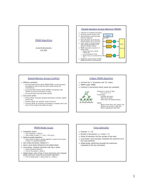
Shared Memory <strong>Access</strong> Conflicts<br />
Different variations:<br />
Exclusive Read Exclusive Write (EREW) <strong>PRAM</strong>: no two processors<br />
are allowed to read or write the same shared memory cell<br />
simultaneously<br />
Concurrent Read Exclusive Write (CREW): simultaneous read<br />
allowed, but only one processor can write<br />
Concurrent Read Concurrent Write (CRCW)<br />
Concurrent writes:<br />
Priority CRCW: processors assigned fixed distinct priorities, highest<br />
priority wins<br />
Arbitrary CRCW: one randomly chosen write wins<br />
Common CRCW: all processors are allowed to complete write if and<br />
only if all the values to be written are equal<br />
Complexity issues:<br />
Time complexity = O(log n)<br />
<strong>PRAM</strong> Model Issues<br />
Total number of steps = n * log n = O(n log n)<br />
Optimal parallel algorithm:<br />
Total number of steps in parallel algorithm is equal to the number<br />
of steps in a sequential algorithm<br />
Use n/logn processors instead of n<br />
Have a local phase followed by the global phase<br />
Local phase: compute maximum over log n values<br />
Simple sequential algorithm<br />
Time for local phase = O(log n)<br />
Global phase: take (n/log n) local maximums and compute<br />
global maximum using the tournament algorithm<br />
Time for global phase = O(log (n/log n)) = O(log n)<br />
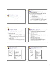
<strong>Parallel</strong> <strong>Random</strong> <strong>Access</strong> <strong>Machine</strong> (<strong>PRAM</strong>)<br />
Collection of numbered processors<br />
<strong>Access</strong>ing shared memory cells<br />
Each processor could have local<br />
memory (registers)<br />
Each processor can access any<br />
shared memory cell in unit time<br />
Input stored in shared memory<br />
cells, output also needs to be<br />
stored in shared memory<br />
<strong>PRAM</strong> instructions execute in 3phase<br />
cycles<br />
Read (if any) from a shared<br />
memory cell<br />
Local computation (if any)<br />
Write (if any) to a shared memory<br />
cell<br />
Processors execute these 3-phase<br />
<strong>PRAM</strong> instructions synchronously<br />
Control<br />
Private<br />
Memory<br />
Private<br />
Memory<br />
Private<br />
Memory<br />
A Basic <strong>PRAM</strong> Algorithm<br />
Let there be “n” processors and “2n” inputs<br />
<strong>PRAM</strong> model: EREW<br />
Construct a tournament where values are compared<br />
P0<br />
v P0<br />
P0 P2 P4<br />
P4<br />
P6<br />
P0 P1 P2 P3 P4 P5 P6 P7<br />
Example: n = 16<br />
Processor k is active in step j<br />
if (k % 2 j ) == 0<br />
At each step:<br />
Compare two inputs,<br />
Take max of inputs,<br />
Write result into shared memory<br />
P 1<br />
P 2<br />
P p<br />
Global<br />
Memory<br />
Details:<br />
Need to know who is the “parent” and<br />
whether you are left or right child<br />
Write to appropriate input field<br />
Time Optimality<br />
Number of processors, p = n/log n = 4<br />
Divide 16 elements into four groups of four each<br />
Local phase: each processor computes the maximum of its<br />
four local elements<br />
Global phase: performed amongst the maximums<br />
computed by the four processors<br />
1
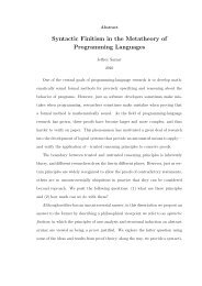
Finding Maximum: CRCW Algorithm Broadcast and reduction<br />
Broadcast of 1 value to p processors in log p time<br />
Given n elements A[0, n-1], find the maximum.<br />
With n 2 processors, each processor (i,j) compare A[i] and A[j], for 0≤ i, j ≤n-1.<br />
FAST-MAX(A):<br />
1. n←length[A]<br />
2. for i ←0 to n-1, in parallel<br />
3. do m[i] ←true<br />
4. for i ←0 to n-1 and j ←0 to n-1, in parallel<br />
5. do if A[i] < A[j]<br />
6. then m[i] ←false<br />
7. for i ←0 to n-1, in parallel<br />
8. do if m[i] =true<br />
9. then max ← A[i]<br />
10. return max<br />
A[i]<br />
The running time is O(1).<br />
Note: there may be multiple maximum values, so their processors<br />
Will write to max concurrently. Its work = n 2 × O(1) =O(n 2 ).<br />
Scan (or <strong>Parallel</strong> prefix)<br />
A[j]<br />
5 6 9 2 9 m<br />
5 F T T F T F<br />
6 F F T F T F<br />
9 F F F F F T<br />
2 T T T F T F<br />
9 F F F F F T<br />
max=9<br />
What if you want to compute partial sums<br />
Definition: the parallel prefix operation take a binary<br />
associative operator , and an array of n elements<br />
[a 0, a 1, a 2, … a n-1]<br />
and produces the array<br />
[a 0, (a 0 a 1), … (a 0 a 1 ... a n-1)]<br />
Example: add scan of<br />
[1, 2, 0, 4, 2, 1, 1, 3] is [1, 3, 3, 7, 9, 10, 11, 14]<br />
Can be implemented in O(n) time by a serial algorithm<br />
Obvious n-1 applications of operator will work<br />
Up sweep:<br />
Tree summation 2 phases<br />
up sweep<br />
mine = left<br />
Implementing Scans<br />
get values L and R from left and right child<br />
save L in local variable Mine<br />
compute Tmp = L + R and pass to parent<br />
down sweep<br />
get value Tmp from parent<br />
send Tmp to left child<br />
send Tmp+Mine to right child<br />
tmp = left + right<br />
6<br />
6<br />
9<br />
4<br />
5<br />
4<br />
5 4<br />
3 2 4 1<br />
3 1 2 0 4 1 1 3<br />
Down sweep:<br />
tmp = parent (root is 0)<br />
right = tmp + mine<br />
0<br />
0<br />
4<br />
4<br />
6<br />
6<br />
5<br />
6 11<br />
3 2 4 1<br />
0 3 4 6 6 10 11 12<br />
+X = 3 1 2 0 4 1 1 3<br />
3 4 6 6 10 11 12 15<br />
v<br />
Reduction of p values to 1 in log p time<br />
Takes advantage of associativity in +,*, min, max, etc.<br />
1 3 1 0 4 -6 3 2<br />
8<br />
Broadcast<br />
Add-reduction<br />
Prefix Sum in <strong>Parallel</strong><br />
Algorithm: 1. Pairwise sum 2. Recursively Prefix 3. Pairwise Sum<br />
1 2 3 4 5 6 7 8 9 10 11 12 13 14 15 16<br />
3 7 11 15 19 23 27 31<br />
(Recursively Prefix)<br />
3 10 21 36 55 78 105 136<br />
1 3 6 10 15 21 28 36 45 55 66 78 91 105 120 136<br />
E.g., Using Scans for Array Compression<br />
Given an array of n elements<br />
[a 0, a 1, a 2, … a n-1]<br />
and an array of flags<br />
[1,0,1,1,0,0,1,…]<br />
compress the flagged elements<br />
[a 0, a 2, a 3, a 6, …]<br />
Compute a “prescan” i.e., a scan that doesn’t include the<br />
element at position i in the sum<br />
[0,1,1,2,3,3,4,…]<br />
Gives the index of the i th element in the compressed array<br />
If the flag for this element is 1, write it into the result array at the<br />
given position<br />
2
E.g., Fibonacci via Matrix Multiply Prefix<br />
Fn<br />
⎜<br />
⎝ F<br />
⎛ + 1<br />
F n+1 = F n + F n-1<br />
n<br />
⎞ ⎛1<br />
⎟ = ⎜<br />
⎠ ⎝1<br />
1⎞<br />
⎛ F<br />
⎟ ⎜<br />
0⎠<br />
⎝Fn<br />
n<br />
-1<br />
⎞<br />
⎟<br />
⎠<br />
Can compute all F n by matmul_prefix on<br />
⎛1<br />
1⎞<br />
⎛1<br />
1⎞<br />
⎛1<br />
1⎞<br />
⎛1<br />
1⎞<br />
⎛1<br />
1⎞<br />
⎛1<br />
1⎞<br />
⎛1<br />
1⎞<br />
⎛1<br />
1⎞<br />
⎛1<br />
1⎞<br />
⎜ ⎟ ⎜ ⎟ ⎜ ⎟ ⎜ ⎟ ⎜ ⎟ ⎜ ⎟ ⎜ ⎟ ⎜ ⎟ ⎜ ⎟<br />
[ ⎜1<br />
0⎟,<br />
⎜1<br />
0⎟,<br />
⎜1<br />
0⎟,<br />
⎜1<br />
0⎟,<br />
⎜1<br />
0⎟<br />
, ⎜1<br />
0⎟<br />
, ⎜1<br />
0⎟,<br />
⎜1<br />
0⎟,<br />
⎜1<br />
0⎟<br />
]<br />
⎝<br />
⎠ ⎝<br />
⎠<br />
⎝<br />
then select the upper left entry<br />
⎠<br />
⎝<br />
⎠ ⎝<br />
⎠<br />
⎝<br />
⎠<br />
⎝<br />
⎠ ⎝<br />
⎠<br />
⎝<br />
⎠<br />
Slide source: Alan Edelman, MIT<br />
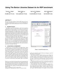
List ranking –EREW algorithm<br />
LIST-RANK(L) (in O(lg n) time)<br />
1. for each processor i, in parallel<br />
2. do if next[i]=nil<br />
3. then d[i]←0<br />
4. else d[i]←1<br />
5. while there exists an object i such that next[i]≠nil<br />
6. do for each processor i, in parallel<br />
7. do if next[i]≠nil<br />
8. then d[i]← d[i]+ d[next[i]]<br />
9. next[i] ←next[next[i]]<br />
Recap<br />
<strong>PRAM</strong> algorithms covered so far:<br />
Finding max on EREW and CRCW models<br />
Time optimal algorithms: number of steps in parallel program is<br />
equal to the number of steps in the best sequential algorithm<br />
Always qualified with the maximum number of processors that<br />
can be used to achieve the parallelism<br />
Reduction operation:<br />
Takes a sequence of values and applies an associative operator<br />
on the sequence to distill a single value<br />
Associative operator can be: +, max, min, etc.<br />
Can be performed in O(log n) time with up to O(n/log n) procs<br />
Broadcast operation: send a single value to all processors<br />
Also can be performed in O(log n) time with up to O(n/log n)<br />
procs<br />
Pointer Jumping –list ranking<br />
Given a single linked list L with n objects, compute,<br />
for each object in L, its distance from the end of the<br />
list.<br />
Formally: suppose next is the pointer field<br />
D[i] = 0 if next[i] = nil<br />
d[next[i]]+1 if next[i] ≠ nil<br />
Serial algorithm: Θ(n)<br />
(a)<br />
List-ranking –EREW algorithm<br />
3<br />
1<br />
4<br />
1<br />
6<br />
1<br />
3 4 6 1 0 5<br />
(b) 2 2 2 2 1 0<br />
3 4 6 1 0 5<br />
(c) 4 4 3 2 1 0<br />
3 4 6 1 0 5<br />
(d) 5 4 3 2 1 0<br />
Used to compute partial sums<br />
1<br />
1<br />
Scan Operation<br />
Definition: the parallel prefix operation take a binary associative<br />
operator , and an array of n elements<br />
[a 0, a 1, a 2, … a n-1]<br />
and produces the array<br />
[a 0, (a 0 a 1), … (a 0 a 1 ... a n-1)]<br />
0<br />
1<br />
Scan(a, n):<br />
if (n == 1) { s[0] = a[0]; return s; }<br />
for (j = 0 … n/2-1)<br />
x[j] = a[2*j] a[2*j+1];<br />
y = Scan(x, n/2);<br />
for odd j in {0 … n-1}<br />
s[j] = y[j/2];<br />
for even j in {0 … n-1}<br />
s[j] = y[j/2] a[j];<br />
return s;<br />
5<br />
0<br />
3
Work-Time Paradigm<br />
Associate two complexity measures with a parallel<br />
algorithm<br />
S(n): time complexity of a parallel algorithm<br />
Total number of steps taken by an algorithm<br />
W(n): work complexity of the algorithm<br />
Total number of operations the algorithm performs<br />
W j (n): number of operations the algorithm performs in step j<br />
W(n) = Σ W j (n) where j = 1…S(n)<br />
Can use recurrences to compute W(n) and S(n)<br />
Brent’s Scheduling Principle<br />
A parallel algorithm with step complexity S(n) and work<br />
complexity W(n) can be simulated on a p-processor <strong>PRAM</strong><br />
in no more than T C(n,p) = W(n)/p + S(n) parallel steps<br />
S(n) could be thought of as the length of the “critical path”<br />
Some schedule exists; need some online algorithm for dynamically<br />
allocating different numbers of processors at different steps of the<br />
program<br />
No need to give the actual schedule; just design a parallel algorithm<br />
and give its W(n) and S(n) complexity measures<br />
Goals:<br />
Design algorithms with W(n) = T S(n), running time of sequential<br />
algorithm<br />
Such algorithms are called work-efficient algorithms<br />
Also make sure that S(n) = poly-log(n)<br />
Speedup = T S(n) / T C(n,p)<br />
Inputs = Ordered Pairs<br />
(operand, boolean)<br />
e.g. (x, T) or (x, F)<br />
Segmented Operations<br />
+ 2 (y, T) (y, F)<br />
(x, T) (x + y, T) (y, F)<br />
(x, F) (y, T) (x⊕y, F)<br />
e. g. 1 2 3 4 5 6 7 8<br />
Result<br />
Change of<br />
segment indicated<br />
by switching T/F<br />
T T F F F T F T<br />
1 3 3 7 12 6 7 8<br />
Recurrences for Scan<br />
Scan(a, n):<br />
if (n == 1) { s[0] = a[0]; return s; }<br />
for (j = 0 … n/2-1)<br />
x[j] = a[2*j] a[2*j+1];<br />
y = Scan(x, n/2);<br />
for odd j in {0 … n-1}<br />
s[j] = y[j/2];<br />
for even j in {0 … n-1}<br />
s[j] = y[j/2] a[j];<br />
return s;<br />
W(n) = 1 + n/2 + W(n/2) + n/2 + n/2 + 1<br />
= 2 + 3n/2 + W(n/2)<br />
S(n) = 1 + 1 + S(n/2) + 1 + 1 = S(n/2) + 4<br />
Solving, W(n) = O(n); S(n) = O(log n)<br />
Application of Brent’s Schedule to Scan<br />
Scan complexity measures:<br />
W(n) = O(n)<br />
S(n) = O(log n)<br />
T C(n,p) = W(n)/p + S(n)<br />
If p equals 1:<br />
T C (n,p) = O(n) + O(log n) = O(n)<br />
Speedup = T S (n) / T C (n,p) = 1<br />
If p equals n/log(n):<br />
T C (n,p) = O(log n)<br />
Speedup = T S (n) / T C (n,p) = n/logn<br />
If p equals n:<br />
T C (n,p) = O(log n)<br />
Speedup = n/logn<br />
Scalable up to n/log(n) processors<br />
<strong>Parallel</strong> prefix on a list<br />
A prefix computation is defined as:<br />
Input: <br />
Binary associative operation ⊗<br />
Output: <br />
Such that:<br />
y 1= x 1<br />
y k= y k-1 ⊗ x k for k= 2, 3, …, n, i.e, y k= ⊗ x 1 ⊗ x 2 …⊗ x k .<br />
Suppose are stored orderly in a list.<br />
Define notation: [i,j]= x i ⊗ x i+1 …⊗ x j<br />
4
LIST-PREFIX(L)<br />
Prefix computation<br />
1. for each processor i, in parallel<br />
2. do y[i]← x[i]<br />
3. while there exists an object i such that prev[i]≠nil<br />
4. do for each processor i, in parallel<br />
5. do if prev[i]≠nil<br />
6. then y[prev[i]]← y[i] ⊗ y[prev[i]]<br />
7. prev[i] ← prev[prev[i]]<br />
Readings:<br />
Announcements<br />
Lecture notes from Sid Chatterjee and Jans Prins<br />
Prefix scan applications paper by Guy Blelloch<br />
Lecture notes from Ranade (for list ranking algorithms)<br />
Homework:<br />
First theory homework will be on website tonight<br />
To be done individually<br />
TA office hours will be posted on the website soon<br />
Optimizing List Prefix<br />
4 3 6 7 4 3<br />
Eliminate some elements:<br />
4 3 9 7 11 3<br />
Perform list prefix on remainder:<br />
4 3 13 7 24 27<br />
Integrate eliminated elements:<br />
4 7 13 20 24 27<br />
What is S(n)?<br />
What is W(n)?<br />
List Prefix Operations<br />
What is speedup on n/logn processors?<br />
List Prefix<br />
4 3 6 7 4 3<br />
4 7 9 13 11 7<br />
4 7 13 20 20 20<br />
4 7 13 20 24 27<br />
<strong>Random</strong>ized algorithm:<br />
Goal: achieve W(n) = O(n)<br />
Sketch of algorithm:<br />
Optimizing List Prefix<br />
1. Select a set of list elements that are non adjacent<br />
2. Eliminate the selected elements from the list<br />
3. Repeat steps 1 and 2 until only one element remains<br />
4. Fill in values for the elements eliminated in preceding steps in the<br />
reverse order of their elimination<br />
5
Optimizing List Prefix<br />
4 3 6 7 4 3<br />
Eliminate #1:<br />
4 3 9 7 11 3<br />
Eliminate #2:<br />
4 3 13 7 11 14<br />
Eliminate #3:<br />
4 3 13 7 11 27<br />
Find root –CREW algorithm<br />
Suppose a forest of binary trees, each node i has a pointer<br />
parent[i].<br />
Find the identity of the tree of each node.<br />
Assume that each node is associated a processor.<br />
Assume that each node i has a field root[i].<br />
Elimination step:<br />
<strong>Random</strong>ized List Ranking<br />
Each processor is assigned O(log n) elements<br />
Processor j is assigned elements j*logn … (j+1)*logn –1<br />
Each processor marks the head of its queue as a candidate<br />
Each processor flips a coin and stores the result along with the<br />
candidate<br />
A candidate is eliminated if its coin is a HEAD and if it so happens<br />
that the previous element is not a TAIL or was not a candidate<br />
FIND-ROOTS(F)<br />
Find-roots –CREW algorithm<br />
1. for each processor i, in parallel<br />
2. do if parent[i] = nil<br />
3. then root[i]←i<br />
4. while there exist a node i such that parent[i] ≠ nil<br />
5. do for each processor i, in parallel<br />
6. do if parent[i] ≠ nil<br />
7. then root[i] ← root[parent[i]]<br />
8. parent[i] ← parent[parent[i]]<br />
Pointer Jumping Example Pointer Jumping Example<br />
6
Pointer Jumping Example Analysis<br />
Find roots –CREW vs. EREW<br />
How fast can n nodes in a forest determine their<br />
roots using only exclusive read?<br />
Ω(lg n)<br />
Argument: when exclusive read, a given peace of information can only be<br />
copied to one other memory location in each step, thus the number of locations<br />
containing a given piece of information at most doubles at each step. Looking<br />
at a forest with one tree of n nodes, the root identity is stored in one place initially.<br />
After the first step, it is stored in at most two places; after the second step, it is<br />
Stored in at most four places, …, so need lg n steps for it to be stored at n places.<br />
So CREW: O(lg d) and EREW: Ω(lg n).<br />
If d=2 o(lg n) , CREW outperforms any EREW algorithm.<br />
If d=Θ(lg n), then CREW runs in O(lg lg n), and EREW is<br />
much slower.<br />
Using Euler Tours<br />
Trees = balanced parentheses<br />
Parentheses subsequence corresponding to a subtree is balanced<br />
Parenthesis version: ( ( ) ( ( ) ( ) ) )<br />
Complexity measures:<br />
What is W(n)?<br />
What is S(n)?<br />
Termination detection: When do we stop?<br />
All the writes are exclusive<br />
But the read in line 7 is concurrent, since several nodes<br />
may have same node as parent.<br />
Euler Tours<br />
Technique for fast processing of tree data<br />
Euler circuit of directed graph:<br />
Directed cycle that traverses each edge exactly once<br />
Represent tree by Euler circuit of its directed version<br />
Input:<br />
Depth of tree vertices<br />
L[i] = position of incoming edge into i in euler tour<br />
R[i] = position of outgoing edge from i in euler tour<br />
forall i in 1..n {<br />
A[L[i]] = 1;<br />
A[R[i]] = -1;<br />
}<br />
B = EXCL-SCAN(A, “+”);<br />
forall i in 1..n<br />
Depth[i] = B[L[i]];<br />
Parenthesis version: ( ( ) ( ( ) ( ) ) )<br />
Scan input: 1 1 -1 1 1 -1 1 -1 -1 -1<br />
Scan output: 0 1 2 1 2 3 2 3 2 1<br />
7
Divide and Conquer<br />
Just as in sequential algorithms<br />
Divide problems into sub-problems<br />
Solve sub-problems recursively<br />
Combine sub-solutions to produce solution<br />
Example: planar convex hull<br />
Give set of points sorted by x-coord<br />
Find the smallest convex polygon that contains the points<br />
Overall approach:<br />
Convex Hull<br />
Take the set of points and divide the set into two halves<br />
Assume that recursive call computes the convex hull of the two<br />
halves<br />
Conquer stage: take the two convex hulls and merge it to obtain<br />
the convex hull for the entire set<br />
Complexity:<br />
W(n) = 2*W(n/2) + merge_cost<br />
S(n) = S(n/2) + merge_cost<br />
If merge_cost is O(log n), then S(n) is O(log 2 n)<br />
Merge can be sequential, parallelism comes from the recursive<br />
subtasks<br />
Complex Hull Example Complex Hull Example<br />
Complex Hull Example Complex Hull Example<br />
8
Challenge:<br />
Merge Operation<br />
Finding the upper and lower common tangents<br />
Simple algorithm takes O(n)<br />
We need a better algorithm<br />
Insight:<br />
Resort to binary search<br />
Consider the simpler problem of finding a tangent from a point to a<br />
polygon<br />
Extend this to tangents from a polygon to another polygon<br />
More details in Preparata and Shamos book on Computational<br />
Geometry (Lemma 3.1)<br />
9