Optimetrics: Parametrics and Optimization Using Ansoft HFSS

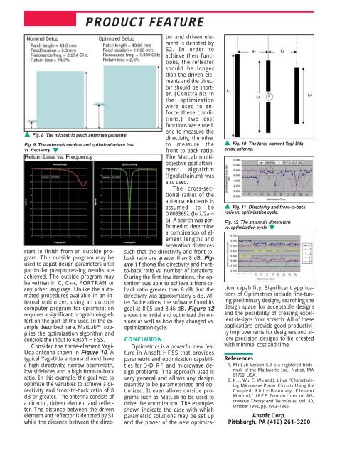
▲ Fig. 8 The microstrip patch antenna’s geometry.
Fig. 9 The antenna’s nominal and optimized return loss
vs. frequency. ▼
start to finish from an outside program.
This outside program may be
used to adjust design parameters until
particular postprocessing results are
achieved. The outside program may
be written in C, C++, FORTRAN or
any other language. Unlike the automated
procedures available in an internal
optimizer, using an outside
computer program for optimization
requires a significant programming effort
on the part of the user. In the example
described here, MatLab supplies
the optimization algorithm and
controls the input to Ansoft HFSS.
Consider the three-element Yagi-
Uda antenna shown in Figure 10. A
typical Yagi-Uda antenna should have
a high directivity, narrow beamwidth,
low sidelobes and a high front-to-back
ratio. In this example, the goal was to
optimize the variables to achieve a directivity
and front-to-back ratio of 8
dB or greater. The antenna consists of
a director, driven element and reflector.
The distance between the driven
element and reflector is denoted by S1
while the distance between the direc-
PRODUCT FEATURE
tor and driven element
is denoted by
S2. In order to
achieve their functions,
the reflector
should be longer
than the driven elements
and the director
should be shorter.
(Constraints in
the optimization
were used to enforce
these conditions.)
Two cost
functions were used:
one to measure the
directivity, the other
to measure the
front-to-back-ratio.
The MatLab multiobjective
goal attainment
algorithm
(fgoalattain.m) was
also used.
The cross-sectional
radius of the
antenna elements is
assumed to be
0.003369λ (ln λ/2a =
5). A search was performed
to determine
a combination of element
lengths and
separation distances
such that the directivity and front-toback
ratio are greater than 8 dB. Figure
11 shows the directivity and frontto-back
ratio vs. number of iterations.
During the first few iterations, the optimizer
was able to achieve a front-toback
ratio greater than 8 dB, but the
directivity was approximately 5 dB. After
34 iterations, the software found its
goal at 8.05 and 8.46 dB. Figure 12
shows the initial and optimized dimensions
as well as how they changed vs.
optimization cycle.
CONCLUSION
Optimetrics is a powerful new feature
in Ansoft HFSS that provides
parametric and optimization capabilities
for 3-D RF and microwave design
problems. The approach used is
very general and allows any design
quantity to be parameterized and optimized.
It even allows outside programs
such as MatLab to be used to
drive the optimization. The examples
shown indicate the ease with which
parametric solutions may be set up
and the power of the new optimiza-
▲ Fig. 10 The three-element Yagi-Uda
array antenna.
▲ Fig. 11 Directivity and front-to-back
ratio vs. optimization cycle.
Fig. 12 The antenna’s dimensions
vs. optimization cycle. ▼
tion capability. Significant applications
of Optimetrics include fine-tuning
preliminary designs, searching the
design space for acceptable designs
and the possibility of creating excellent
designs from scratch. All of these
applications provide good productivity
improvements for designers and allow
precision designs to be created
with minimal cost and time.
References
1. MatLab Version 5.3 is a registered trademark
of the Mathworks Inc., Natick, MA
01760, USA.
2. K.L. Wu, C. Wu and J. Litva, “Characterizing
Microwave Planar Circuits Using the
Coupled Finite-Boundary Element
Method,” IEEE Transactions on Microwave
Theory and Techniques, Vol. 40,
October 1992, pp. 1963–1966.
Ansoft Corp.
Pittsburgh, PA (412) 261-3200