Optimetrics: Parametrics and Optimization Using Ansoft HFSS

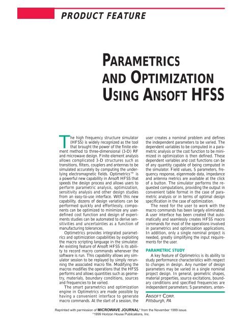
PRODUCT FEATURE
The high frequency structure simulator
(HFSS) is widely recognized as the tool
that brought the power of the finite element
method to three-dimensional (3-D) RF
and microwave design. Finite element analysis
allows complicated 3-D structures such as
transitions, filters, couplers and antennas to be
simulated accurately by computing the underlying
electromagnetic fields. Optimetrics is
a powerful new capability in Ansoft HFSS that
speeds the design process and allows users to
perform parametric analysis, optimization,
sensitivity analysis and other design studies
from an easy-to-use interface. With this new
capability, dozens of design variations can be
performed quickly and effortlessly, components
can be optimized to minimize any userdefined
cost function and design of experiments
studies can be automated to derive sensitivities
and uncertainties as a function of
manufacturing tolerances.
Optimetrics provides integrated parametrics
and optimization capabilities by exploiting
the macro scripting language in the simulator.
An existing feature of Ansoft HFSS is its ability
to record macro commands whenever the
software is run. This capability allows any simulator
session to be replayed by simply rerunning
the associated macro file. Modifying the
macros modifies the operations that the HFSS
performs and allows quantities such as geometry,
materials, boundary conditions, sources
and frequencies to be varied.
The smart parametrics and optimization
engine in Optimetrics are made possible by
having a convenient interface to generate
macro commands. At the start of a session, the
PARAMETRICS
AND OPTIMIZATION
USING ANSOFT HFSS
user creates a nominal problem and defines
the independent parameters to be varied. The
dependent variables to be computed in a parametric
analysis or the cost function to be minimized
in optimization is then defined. These
dependent variables and cost functions can be
of any quantity capable of being computed in
the simulator. Field values, S parameters, frequency
response, eigenmode data, impedance
and antenna metrics are available at the click
of a button. The simulator performs the requested
computations, providing the output in
convenient table format in the case of parametric
analysis or in terms of optimal design
specification in the case of optimization.
The need for the user to work with the
macro commands has been largely eliminated.
A user interface has been created that automatically
and seamlessly creates HFSS macro
commands for most of the operations involved
in parametrics and optimization applications.
In addition, only a single nominal project is
needed, greatly simplifying the input requirements
for the user.
PARAMETRIC STUDY
A key feature of Optimetrics is its ability to
study performance characteristics with respect
to changes in design. Any number of design
parameters may be varied in a single nominal
project design. In general, geometric shapes,
material properties, source excitations, boundary
conditions and specified frequencies are
independent parameters; S parameters, anten-
ANSOFT CORP.
Pittsburgh, PA
Reprinted with permission of MICROWAVE JOURNAL ® from the November 1999 issue.
© 1999 Horizon House Publications, Inc.

na parameters, eigenmode data or
other HFSS-computed quantities are
dependent parameters. Users can
create compound parameters, which
are a function of both dependent and
independent parameters. Such a
compound parameter can be used for
better visualization and understanding
of the project or as a cost function
to be used in the optimizer. The
number of independent or dependent
parameters is unlimited. All dependencies,
such as boundary conditions,
are restored intelligently including
face picks, impedance,
calibration lines, gap source lines and
the UV coordinate system of periodic
boundaries. For example, if an impedance
line has been created that is
one-third wavelength from the end of
a port face, this line will always be
one-third wavelength for the parametric
projects.
Fig. 1 An H-plane reactive T-junction with
inductive septum. ▼
Fig. 2 Optimetrics table for organizing and simulating
parameters. ▼
PRODUCT FEATURE
Consider the problem of computing
the power division produced by an
inductive septum in a waveguide Tjunction
at 10 GHz, as shown in Figure
1. To solve this problem as a
function of the septum offset, the
nominal problem is entered and
solved. With Optimetrics, a table is
set up for sweeping the offset with
each row of the table corresponding
to a specific offset value. (There is no
limit on the number of rows users can
enter.) Taking into account the parameters
specified for the row, solving
the table creates an HFSS project for
every row of the table. Optimetrics
supports automatic seeding for each
parametric setup. In the case where
no geometry parameter is changed,
the refined nominal mesh is used as
the starting mesh for all solutions.
Dependent and compound parameters
can be added as columns of a table.
In this case, the original dependent parameters
of interest are the magnitude
of the scattering parameters. Upon execution,
the value of the dependent parameter
computed for this row’s solution
fills the far right columns as shown
in Figure 2. In this case, the problem
size was 8000 unknowns and required
three minutes and five seconds per row
using a 360 MHz Pentium III processor.
If the user is not satisfied with the
accuracy of the solution, it is possible to
perform additional refinement and obtain
a higher accuracy solution for
every row. Users can also add frequency
sweeps if single frequency
information is insufficient.
Optimetrics offers users the choice
of either saving or deleting the para-
metric field solutions. Turning off the
field-saving feature saves disk space,
but the parametric field solutions are
not available for later viewing. The
values of the dependent parameters
are always retained.
Table postprocessing enables users
to plot one column against another, as
shown in Figure 3. Parametric projects
can be viewed in the same detail
as the nominal project. A macro file
created in the nominal project to
generate plots can be run for any
parametric setup with the click of a
button. The saved plots for every row
can be plotted together to view the
effect of changing parameter values
on the plots.
Even after the solution is completed,
the user may add new solution
columns to the table. In this case, the
left-to-right power ratio vs. offset is
evaluated and plotted. Within seconds,
Optimetrics creates new columns and
fills them by deriving the newly requested
data from the existing solutions
in the corresponding rows. The results
are shown in Figure 4.
Fig. 3 S parameters vs. septum position
for the reactive T-junction. ▼
Fig. 4 New plots of derived quantities. ▼

▲ Fig. 5 A four-post microstrip filter.
▲ Fig. 6 The optimized filter’s frequency response.
Fig. 7 The modeled microstrip
patch antenna. ▼
OPTIMIZATION
Optimetrics contains a powerful
internal optimization algorithm to
help users achieve optimal designs.
This optimizer employs a constrained
superlinearly convergent active set algorithm.
To restrict the search region
and prevent the optimizer from creating
physically meaningless designs
(such as overlapping geometry), Optimetrics
supports simple bounds as
well as linear constraints. The optimized
design is guaranteed to be
within the feasible domain.
Optimetrics also provides users
with unlimited freedom in defining
cost functions for optimization. Any
algebraic expression may be defined
as the cost function and any solution
quantity (such as field strength, far-
PRODUCT FEATURE
field values or circuit parameters that
can be computed in the simulator)
may be used as a variable in this cost
function. Optimetrics searches the
design space to minimize the cost
function. To accommodate maximization
or compound objectives, the user
may construct partial cost functions
and/or apply appropriate weights.
To simplify cost function definition
for standard tasks, Optimetrics provides
a graphical user interface that
allows the user access
to commonly
used quantities
(such as circuit parameters)
with the
push of a button. A
special panel for filter
optimization is
also provided. The
user may choose an
arbitrary number of
frequency bands
and specify the requested
filter characteristics.
Expert
users can even create
their own macro
scripts. The cost functions in the
macro script may contain loops and
conditional statements.
By default, optimization starts from
the nominal settings for the design.
However, if a parametric table is available,
Optimetrics will first scan the
table, analyze all designs that are feasible
and start optimization from the design
of least cost. Hence, the user may
manually create parameter settings for
one or more candidates as the starting
point for the optimization, or even begin
with a parametric sweep. Beginning
with a parametric sweep is particularly
attractive when the user chooses to inspect
the response surface over a wide
range of parameters and may also help
to avoid local optima.
FINE-TUNING A DESIGN
To illustrate some of the productivity
gains afforded by Optimetrics,
consider the problem of fine-tuning
the product design. It often happens
that a designer has the basic parameters
for a microwave component but
needs to fine-tune these parameters
to deliver a precision product. Using
cut-and-try methods, such fine-tuning
can require weeks of prototyping
and tweaking; using Optimetrics, it
can be performed overnight.
Consider the four-post microstrip
bandpass filter shown in Figure 5.
This filter was designed 1 in an attempt
to meet a design goal of an 8 to
9 GHz passband with less than 1 dB
ripple. Using traditional filter design
techniques, a filter was designed, fabricated,
tested and published with a
7.6 to 9 GHz passband and 1.5 dB
ripple. Using the published dimensions
as the nominal design, this filter
was entered into Optimetrics. The
optimization problem consists of four
parameters: the diameter of the end
posts, the diameter of the center
posts, the spacing between the end
and center posts, and the spacing between
the center posts. As shown in
Figure 6, Optimetrics improved this
design considerably; the optimized
design has a passband from 8 to 9
GHz with less than 0.6 dB ripple, exceeding
the design specifications.
CREATING A DESIGN
FROM SCRATCH
In some cases, Optimetrics is able
to create an excellent design even
though the user has little initial
knowledge of a good design. This capability
is not foolproof; complex designs
often have many parameters
and many local minima that can confound
direct optimization. A designer
is advised to perform a parametric
sweep first and must use his or her
judgment to create an initial good design.
Nevertheless, in some simple
cases, the optimizer works surprisingly
well in creating designs with minimal
user design input.
Consider the microstrip patch antenna
in Figure 7. The design goal for
this antenna is to produce an antenna
resonant at 2 GHz and the lowest possible
return loss at resonance. The design
parameters are the length of the
patch and the feed location on the side
of the patch. The nominal patch and
the optimized patch are shown in Figure
8; the corresponding return loss vs.
frequency plots are shown in Figure 9.
In this case it can be seen that the
nominal patch is very far from an acceptable
design while the optimized
patch provides good performance.
OPTIMIZATION USING
EXTERNAL OPTIMIZERS
Since Optimetrics is based on the
HFSS macro scripting language, it is
possible to drive Ansoft HFSS from

▲ Fig. 8 The microstrip patch antenna’s geometry.
Fig. 9 The antenna’s nominal and optimized return loss
vs. frequency. ▼
start to finish from an outside program.
This outside program may be
used to adjust design parameters until
particular postprocessing results are
achieved. The outside program may
be written in C, C++, FORTRAN or
any other language. Unlike the automated
procedures available in an internal
optimizer, using an outside
computer program for optimization
requires a significant programming effort
on the part of the user. In the example
described here, MatLab supplies
the optimization algorithm and
controls the input to Ansoft HFSS.
Consider the three-element Yagi-
Uda antenna shown in Figure 10. A
typical Yagi-Uda antenna should have
a high directivity, narrow beamwidth,
low sidelobes and a high front-to-back
ratio. In this example, the goal was to
optimize the variables to achieve a directivity
and front-to-back ratio of 8
dB or greater. The antenna consists of
a director, driven element and reflector.
The distance between the driven
element and reflector is denoted by S1
while the distance between the direc-
PRODUCT FEATURE
tor and driven element
is denoted by
S2. In order to
achieve their functions,
the reflector
should be longer
than the driven elements
and the director
should be shorter.
(Constraints in
the optimization
were used to enforce
these conditions.)
Two cost
functions were used:
one to measure the
directivity, the other
to measure the
front-to-back-ratio.
The MatLab multiobjective
goal attainment
algorithm
(fgoalattain.m) was
also used.
The cross-sectional
radius of the
antenna elements is
assumed to be
0.003369λ (ln λ/2a =
5). A search was performed
to determine
a combination of element
lengths and
separation distances
such that the directivity and front-toback
ratio are greater than 8 dB. Figure
11 shows the directivity and frontto-back
ratio vs. number of iterations.
During the first few iterations, the optimizer
was able to achieve a front-toback
ratio greater than 8 dB, but the
directivity was approximately 5 dB. After
34 iterations, the software found its
goal at 8.05 and 8.46 dB. Figure 12
shows the initial and optimized dimensions
as well as how they changed vs.
optimization cycle.
CONCLUSION
Optimetrics is a powerful new feature
in Ansoft HFSS that provides
parametric and optimization capabilities
for 3-D RF and microwave design
problems. The approach used is
very general and allows any design
quantity to be parameterized and optimized.
It even allows outside programs
such as MatLab to be used to
drive the optimization. The examples
shown indicate the ease with which
parametric solutions may be set up
and the power of the new optimiza-
▲ Fig. 10 The three-element Yagi-Uda
array antenna.
▲ Fig. 11 Directivity and front-to-back
ratio vs. optimization cycle.
Fig. 12 The antenna’s dimensions
vs. optimization cycle. ▼
tion capability. Significant applications
of Optimetrics include fine-tuning
preliminary designs, searching the
design space for acceptable designs
and the possibility of creating excellent
designs from scratch. All of these
applications provide good productivity
improvements for designers and allow
precision designs to be created
with minimal cost and time.
References
1. MatLab Version 5.3 is a registered trademark
of the Mathworks Inc., Natick, MA
01760, USA.
2. K.L. Wu, C. Wu and J. Litva, “Characterizing
Microwave Planar Circuits Using the
Coupled Finite-Boundary Element
Method,” IEEE Transactions on Microwave
Theory and Techniques, Vol. 40,
October 1992, pp. 1963–1966.
Ansoft Corp.
Pittsburgh, PA (412) 261-3200