Projektpraktikum - TU Graz - Institut für Theoretische Physik ...
Projektpraktikum - TU Graz - Institut für Theoretische Physik ...
Projektpraktikum - TU Graz - Institut für Theoretische Physik ...

Create successful ePaper yourself
Turn your PDF publications into a flip-book with our unique Google optimized e-Paper software.
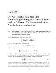
<strong>Projektpraktikum</strong><br />
Technische Universität <strong>Graz</strong><br />
<strong>Institut</strong> <strong>für</strong> <strong>Theoretische</strong> <strong>Physik</strong><br />
Computational Physics<br />
Bose-Einstein Condensation<br />
Advisor:<br />
Univ.-Prof. Dr.rer.nat. Enrico Arrigoni<br />
Daniel Bauernfeind<br />
Mat.Nr. 0730833<br />
Juni 2011
Contents<br />
1 Thermodynamical Basics of the Ideal Bose Gas 5<br />
2 Interacting Bosons 8<br />
2.1 Free particles - Calculating the fluctuations . . . . . . . . . . . 10<br />
2.2 Arbitrary potential V (R) - Multi-Mode Bogoliubov Transfor-<br />
mation . . . . . . . . . . . . . . . . . . . . . . . . . . . . . . . 18<br />
3 Results 25<br />
3.1 Free Particles in 1 Dimension . . . . . . . . . . . . . . . . . . 25<br />
3.2 Particles in a Harmonic Potential . . . . . . . . . . . . . . . . 28<br />
A Substituting the Bogoliubuv approximation into the Hamil-<br />
tonian 35<br />
B Performing the Fourier transformation for the free particles 37<br />
C Proof of conservation of bosonic- commutation relation 39<br />
1
D Calculating the 2L×2L matrix for the multi-mode Bogoliubov<br />
transformation 41<br />
E Derivation of the condition for the commutation relations for<br />
the multi-mode Bogoliubov transformation 44<br />
2
Abstract<br />
In this work an attempt to describe Bose-Einstein Condensation (BCE) for<br />
a 1 dimensional system is made. In chapter 1 a brief introduction to BCE<br />
out of statistical physics can be found.<br />
In chapter 2, starting from the Bose-Hubbard Hamiltonian, a derivation for<br />
the Gross-Pitaevski Equation 2.6 which is one of the central equations for<br />
this description of BCE is done.<br />
With the GPE the problem is solved for free particles in chapter 2.1. There<br />
a Bogoliubov transformation is done, given in equation 2.15. The condi-<br />
tions for this transformation, that the Hamiltonian is diagonal and that the<br />
bosonic commutation relations are conserved, are other important equations<br />
in solving the problem.<br />
Chapter 2.2 finally describes how to solve the problem for an arbitrary poten-<br />
tial V(R) via a Multi-Mode Bogoliubov transformation (MMB transforma-<br />
tion), which is the extension of the Bogoliubov transformation in the previous<br />
chapter. Here, in addition to the GPE also the 2 already mentioned condi-<br />
tions have to be fulfilled.<br />
Results of the two worked out problems can be found in chapter 3.1 and<br />
3.2. Because of the work intensity of the MMB transformation I stopped<br />
at the point where the Hamiltonian was diagonal and didn’t calculate any<br />
properties like I did in the zero potential case.<br />
3
Introduction<br />
When Einstein developed the quantum statistics for indistinguishable parti-<br />
cles, based on a work of the Indian physicist Nathanel Bose, he discovered,<br />
that a dilute gas of such particles can undergo a phase transition named<br />
Bose-Einstein condensation. The fascinating thing about BCE is, that the<br />
strange world of quantum mechanics and its effects actually can be seen by<br />
the pure eye. This makes it interesting from a theoretical as well as from a<br />
experimental point of view.<br />
In this work the problem is solved for a one dimensional lattice using a field<br />
theory approach. In principle, a contradiction occurs due to the mean field<br />
nature of the present approximation: according to the Mermin– Wagner–<br />
Hohenberg theorem which forbids spontaneously broken symmetry in sys-<br />
tems with less than three dimensions. [3]<br />
Nevertheless it is interesting to consider and spend time with such a problem<br />
since it shows a way how to actually solve problems which are more compli-<br />
cated as e.g.: the harmonic oscillator and it gives an insight in the big field<br />
of mean field theory.<br />
4
Chapter 1<br />
Thermodynamical Basics of the<br />
Ideal Bose Gas<br />
The following short introduction to BCE is, concerning the content, a sum-<br />
mary of [2].<br />
We consider noninteracting bosons with zero spin and mass m. The occu-<br />
pation of an energy level with energy ɛp = p2<br />
2m<br />
Einstein-statistics:<br />
〈np〉 = ¯np =<br />
with the inverse temperature β = 1<br />
kbT<br />
1<br />
e β(ɛp−µ) − 1<br />
Hence the total particle number is given by:<br />
N = <br />
¯np = N0 + <br />
¯np<br />
p<br />
is then given by the Bose-<br />
, (1.1)<br />
and the chemical potential µ.<br />
p=0<br />
(1.2)<br />
From equation 1.1 we can see, that the chemical potential µ has to be<br />
smaller than the smallest energy ɛp, which can be taken zero without loss<br />
of generality. If the chemical potential approaches this smallest energy the<br />
5
occupation of the ground state N0 → ∞. Because of this problem we from<br />
now on treat it separately.<br />
For ɛp − µ > 0 we can expand 1.1 as a Taylor series:<br />
¯np =<br />
∞<br />
l=1<br />
<br />
e −β(ɛp−µ)<br />
l The total particle number is then given by:<br />
N = N0 + V<br />
(2π) 3<br />
∞<br />
e βµl<br />
<br />
l=1<br />
(1.3)<br />
e − p2 l<br />
2mk b T d 3 p (1.4)<br />
Where we already replaced the sum over all discrete states by an integral<br />
<br />
3 · · · d p. This integral can be solved easily and leads to:<br />
V<br />
(2π) 3<br />
N = N0 + V<br />
λ 3<br />
∞<br />
l=1<br />
with the thermal de Broglie wavelength λ =<br />
eβµl l3/2 = N0 + V<br />
λ3 g3/2(e βµ ) , (1.5)<br />
and the generalized<br />
√ 2π<br />
2πmkbT<br />
zeta-function g3/2(eβµ ). For a given particle number, equation 1.5 deter-<br />
mines the chemical potential µ. At high temperatures T → ∞, the chemical<br />
potential has to approach −∞. For lower temperatures, on the other hand, it<br />
has to approach zero. Equivalent to the chemical potential approaching zero<br />
the limit for e βµ → 1 can be taken. Then the generalized zeta function can be<br />
replaced by the Riemann zeta function ζ(3/2). As seen above the chemical<br />
potential cannot be positive, why there has to be a certain temperature Tc<br />
where µ = 0 for T < Tc. When the temperature exceeds this critical temper-<br />
ature the number of particles in the ground state is still N0 = O(1) and can<br />
be neglected. With this condition we can calculate the critical temperature<br />
from equation 1.5:<br />
6
kBTc = 2π2<br />
3/2 N<br />
m ζ(3/2)V<br />
(1.6)<br />
For temperatures lower than Tc the fraction of particles in the ground<br />
state or condensed particles can be calculated from 1.5 as:<br />
N0<br />
N<br />
<br />
T<br />
= 1 −<br />
Tc<br />
3/2<br />
(1.7)<br />
This means, that at a temperature lower than Tc a macroscopic amount<br />
of particles occupies the ground state and the fraction of condensed particles<br />
approaches one as T becomes zero. On the other hand for temperatures<br />
higher than Tc the number of condensed particles can be neglected.<br />
7
Chapter 2<br />
Interacting Bosons<br />
We now consider a simple model for interacting bosons described by the one<br />
dimensional Bose-Hubbard-Hamiltonian:<br />
H =<br />
L<br />
(V (R) − µ) ˆ ψ †<br />
R ˆ ψR − t<br />
R=1<br />
L<br />
R=1<br />
<br />
ˆψ †<br />
R ˆ ψR+1 + ˆ ψR ˆ ψ †<br />
<br />
R+1 + U<br />
2<br />
L<br />
( ˆ ψ †<br />
R=1<br />
R )2 ( ˆ ψR) 2 .<br />
(2.1)<br />
Where the first term corresponds to an external potential, which in this work<br />
is chosen to be: V (R) = α(R − L<br />
2 )2 . This term also contains the chemical<br />
potential, which insures particle conservation. The second term describes<br />
the movement of the particles, where just hopping from a lattice point to<br />
its nearest neighbors is included. The last part is the interaction potential<br />
between 2 particles, where the potential V (R − R ′ ) acts only on particles on<br />
the same site:<br />
The bosonic field-operators ˆ ψR and ψ †<br />
R<br />
relations:<br />
V (R − R ′ ) = UδRR ′ . (2.2)<br />
8<br />
obey the bosonic commutation
[ψ(R ′ ), ψ(R) † ] = δR,R ′<br />
[ψ(R ′ ) † , ψ(R) † ] = 0<br />
[ψ(R ′ ), ψ(R)] = [ψ(R ′ ) † , ψ(R) † ] = 0 .<br />
(2.3)<br />
In the condensed phase these are split into a term φ(R) describing the<br />
condensate and one operator ˆ bR which treats the fluctuation around this<br />
value [4, p. 350].<br />
ˆψR = φ(R) + ˆ bR<br />
ˆψ †<br />
R = φ(R) + ˆ b †<br />
R .<br />
(2.4)<br />
Where φ(R) is a real number, not an operator. A problem with that ap-<br />
proach is, that it violates particle conservation, since ˆ ψR acting on a vector<br />
destroys a particle at R. The number φ(R) however leaves the state un-<br />
changed.<br />
Substituting 2.4 into the Hamiltonian 2.1 leads to 1 :<br />
1 See Appendix A for detailed calculation.<br />
9
H = <br />
<br />
(V (R) − µ)|φ(R)|<br />
R<br />
2 + U<br />
2 |φ(R)|4 <br />
− 2tφ(R + 1)φ(R) +<br />
<br />
ˆbR (V (R) − µ)φ(R) + U|φ(R)| 2 <br />
φ(R) − t(φ(R − 1) + φ(R + 1)) +<br />
<br />
ˆ† b R (V (R) − µ)φ(R) + U|φ(R)| 2 <br />
φ(R) − t(φ(R − 1) + φ(R + 1)) +<br />
ˆ† b R ˆ <br />
bR (V (R) − µ) + 2U|φ(R)| 2<br />
<br />
+ U<br />
2 φ(R)2<br />
<br />
ˆ2 bR + ˆ (b †<br />
R )2<br />
<br />
− t<br />
<br />
U<br />
2(<br />
2<br />
ˆb †<br />
R )2ˆbRφ(R) + 2ˆb †<br />
R ˆb 2 Rφ(R) + ( ˆb †<br />
R )2ˆ <br />
2<br />
bR .<br />
(2.5)<br />
ˆ b †<br />
R ˆ bR+1 + ˆ bR ˆ b †<br />
R+1<br />
Because of the Hamiltonian being stationary in the operators ˆ bR and ˆ b †<br />
R ,<br />
the terms linear in these have to vanish. This leads to the Gross-Pitaevskii<br />
equation (GPE), which can be used to determine the condensate amplitude<br />
φ(R):<br />
<br />
(V (R) − µ) + U|φ(R)| 2 <br />
) φ(R) − t(φ(R + 1) + φ(R − 1)) = 0 . (2.6)<br />
2.1 Free particles - Calculating the fluctua-<br />
tions<br />
It has to be emphasized that the general approach made in this chapter is not<br />
my idea and can be found a variety of literature e.g.: [4]. All the calculations<br />
for this specific problem on the other hand were done by myself.<br />
The GPE determines the condensate density on lattice site R, |φ(R)| 2 .<br />
Despite that, the size of fluctuations around this value is interesting. There-<br />
10<br />
<br />
+
fore it’s the next step to solve this problem by including terms up to the<br />
second order in the annihilation and creation operators ˆ bR and ˆ b †<br />
R .<br />
To simplify the problem it is first solved for free particles, where V (R) ≡ 0.<br />
With that there is no dependency on R in the Hamiltonian and therefore the<br />
average occupation of the lattice is also independent of the lattice site. This<br />
means φ(R) is the same for all R and from now on it will simply be written<br />
as φ. Consequently the GPE reads:<br />
or<br />
<br />
U|φ| 2 <br />
− µ φ − 2tφ = 0 , (2.7)<br />
|φ| 2 =<br />
2t + µ<br />
U<br />
. (2.8)<br />
With the condensate density |φ| 2 being the same on every place, an ex-<br />
pression for the chemical potential can be found:<br />
µ = N<br />
L U − 2t = nU − 2t , (2.9)<br />
with N the total number of particles and n the particle density.<br />
With 2.8 the Hamiltonian 2.5 simplifies to:<br />
H = <br />
<br />
− µ|φ|<br />
R<br />
2 + U<br />
2 |φ|4 − 2tφ 2<br />
<br />
+<br />
ˆ† b R ˆ <br />
bR − µ + 2U|φ| 2<br />
<br />
+ U<br />
2 φ2ˆ 2<br />
bR + U<br />
2 φ2ˆ †<br />
(b R )2 <br />
− t ˆ† b R ˆbR+1 + ˆbR ˆb †<br />
<br />
R+1 ,<br />
(2.10)<br />
Here, terms of third and fourth order in the fluctuation operators have<br />
been neglected, what is correct in the low density limit.<br />
11
2.10 can be written as:<br />
H = C + <br />
R<br />
Aˆb †<br />
R ˆ <br />
bR + B ˆ2 bR + ˆ (b †<br />
R )2<br />
<br />
− t ˆ† b R ˆbR+1 + ˆbR ˆb †<br />
<br />
R+1 , (2.11)<br />
with the position independent constants:<br />
C = <br />
<br />
R<br />
− µφ 2 + U<br />
2 φ4 − 2tφ 2<br />
<br />
= L(µ + 2t)(µ − 2t)<br />
A = −µ + 2Uφ 2 = µ + 4t<br />
B = U<br />
2 φ2 = t + µ<br />
2 .<br />
2U<br />
(2.12)<br />
Now the creation and annihilation operators are expanded into the basis of<br />
the free particle (in other words, we perform a Fourier transformation):<br />
ˆ bR = 1<br />
√ L<br />
b † 1<br />
R = √<br />
L<br />
<br />
k<br />
<br />
k<br />
e ikRˆ bk<br />
e −ikRˆ b †<br />
k .<br />
(2.13)<br />
Because of the periodic boundary conditions k is restricted to k = 2πn<br />
, n ∈<br />
L<br />
N . Normally n would be chosen to be in [0, L − 1], in this work however<br />
it is convenient to take n symmetric from [− L−1<br />
2<br />
L−1 , ] if L is odd or from<br />
2<br />
[− L L , − 1] if it is even.<br />
2 2<br />
Substituting the Fourier transformation into the Hamiltonian 2.11 leads to2 :<br />
H = C + <br />
(A − 2t cos k) ˆb †<br />
k ˆ <br />
bk + B<br />
k<br />
2 See Appendix B for detailed calculation.<br />
12<br />
ˆ bk ˆ b−k + ˆ b †<br />
k ˆ b †<br />
−k<br />
<br />
. (2.14)
The goal, to diagonalize this Hamiltonian, will be achieved by using a<br />
Bogoliubov transformation:<br />
ˆbk = ukâk + vkâ †<br />
−k<br />
ˆ† b k = u∗kâ †<br />
k + v∗ kâ−k<br />
ˆb−k = u−kâ−k + v−kâ †<br />
k<br />
ˆ† b −k = u∗−kâ †<br />
−k + v∗ −kâk<br />
(2.15)<br />
The parameters uk and vk have to be determined in a way that, assuming<br />
one set of operators already obeys the commutation relation 2.3 (this operators<br />
will be âk and â †<br />
) also obeys it. The last<br />
k ), the other set (ˆbk and b †<br />
k<br />
requirement for the coefficients will be that the Hamiltonian gets diagonal.<br />
Nevertheless this turns out to be possible only for indices k = 0, because for<br />
k = 0:<br />
(A − 2t) ˆb †<br />
0 ˆ <br />
b0 + B ˆb0 ˆb0 + ˆb †<br />
0 ˆb †<br />
<br />
0<br />
(µ + 2t) ˆ b †<br />
0 ˆ b0 +<br />
µ + 2t<br />
2<br />
=<br />
<br />
ˆb0 ˆb0 + ˆb †<br />
0 ˆb †<br />
<br />
0 .<br />
A Bogoliubov transformation is for such an arrangement of coefficients not<br />
possible. This can also be seen by looking at equation 2.21 where k = 0<br />
would lead to a singularity, because of dividing by zero.<br />
The state k = 0 corresponds to the ground state where in 2.4 the creation<br />
and annihilation operators have been replaced by the condensate amplitude<br />
φ(R), where <br />
R |φ(R)|2 = N0.<br />
Since we are interested in BEC, where a big fraction of particles is in the<br />
ground state, there is no big difference between the Fock-states:<br />
13
ˆ b0|N0, N1, ...〉 = N0|N0 − 1, N1, ...〉<br />
ˆ b †<br />
0|N0, N1, ...〉 = N0 + 1|N0 + 1, N1, ...〉<br />
(2.16)<br />
Here the above mentioned violation of particle conservation can be seen:<br />
The replacement of the operators by a number leads to a violation of parti-<br />
cle conservation. For that reason we work in the grand-canonical ensemble<br />
and ensure particle conservation by introducing the chemical potential as a<br />
Lagrange multiplier [3, p. 23].<br />
The Bogoliubov transformation is now done for all indices except k = 0.<br />
First the numbers uk and vk are chosen to be real. Then the commutator<br />
[ ˆbk, ˆb †<br />
k ] is calculated and it is assumed, that âk and â †<br />
k already are bosonic<br />
operators:<br />
[ ˆbk, ˆb †<br />
k ] = u2k[âk, â †<br />
k ] + v2 k[â †<br />
−k , â−k]<br />
<br />
+ ukvk [âk, â−k] + [â †<br />
−k , â†<br />
k ]<br />
<br />
= u 2 k − v 2 k<br />
!<br />
= 1 .<br />
Now the commutator [bk, b−k] is calculated which has to vanish:<br />
[ ˆbk, ˆb−k] = uku−k[âk, â−k] + vkv−k[â †<br />
k , â†<br />
−k ] + [âk, â †<br />
k ]<br />
<br />
<br />
ukv−k − u−kvk<br />
= ukv−k − u−kvk<br />
!<br />
= 0<br />
This condition can be fulfilled by:<br />
14<br />
(2.17)<br />
(2.18)
vk = v−k<br />
uk = u−k .<br />
(2.19)<br />
Plugging the Bogoliubov transformation 2.15 into the Hamiltonian 2.14<br />
leads to:<br />
H =C + 3<br />
(µ + 2t)N0<br />
2<br />
<br />
<br />
u 2 <br />
k(A − 2t cos k) + Bukvk<br />
k=0<br />
<br />
k=0<br />
<br />
k=0<br />
<br />
k=0<br />
â †<br />
k âk<br />
+ Bukvkâ †<br />
−k â−k+<br />
âkâ †<br />
kBukvk + â−kâ †<br />
<br />
−k v 2 <br />
k(A − 2t cos k) + Bukvk +<br />
â †<br />
k↠<br />
−k (A − 2t cos k)ukvk + B(v 2 k + u 2 <br />
k) +<br />
âkâ−k<br />
<br />
(A − 2t cos k)ukvk + B(v 2 k + u 2 <br />
k)<br />
(2.20)<br />
To get rid of the restrictions to the sums u0 = v0 = 0 can be defined,<br />
because with that the sum can again be over all allowed k values.<br />
Demanding the Hamiltonian to be diagonal, uk and vk have to satisfy the<br />
equation:<br />
(A − 2t cos k)ukvk + B(v 2 k + u 2 k) = 0<br />
(A − 2t cos k)vk<br />
<br />
1 + v 2 k + B(2v2 k + 1) = 0 ,<br />
where condition 2.17 was used to get to the second line.<br />
Hence the coefficients uk,vk for the transformation for all k = 0 are given by:<br />
15
vk = − 1<br />
2 +<br />
(µ + 4t − 2t cos k)<br />
2 (µ + 4t − 2t cos k) 2 − (2t + µ) 2<br />
<br />
1<br />
uk =<br />
2 +<br />
(µ + 4t − 2t cos k)<br />
2 (µ + 4t − 2t cos k) 2 − (2t + µ) 2<br />
u−k = uk<br />
v−k = vk<br />
(2.21)<br />
To diagonalize the Hamiltonian 2.20 we use the bosonic commutation relation<br />
and replace âkâ †<br />
k<br />
<br />
H =<br />
k<br />
with 1 + â†<br />
k âk:<br />
C + v 2 <br />
k(A − 2t cos k) + 2Bukvk + 3<br />
(µ + 2t)N0<br />
2<br />
<br />
<br />
u 2 <br />
k(A − 2t cos k) + 2Bukvk<br />
<br />
k<br />
â †<br />
k âk<br />
â †<br />
−kâ−k <br />
v 2 <br />
k(A − 2t cos k) + 2Bukvk<br />
(2.22)<br />
Because of the allowed values for k, and the coefficients at the creation and<br />
annihilation operators in the second line of 2.22 being symmetric around zero<br />
3 the Hamiltonian can be simplified to:<br />
<br />
H =<br />
C + v 2 k(A − 2t cos k) + 2Bukvk<br />
<br />
k<br />
â †<br />
k âk<br />
<br />
+<br />
<br />
(u 2 k + v 2 k)(A − 2t cos k) + 4Bukvk<br />
(2.23)<br />
The minimum energy is obtained by setting all excitations â †<br />
k âk = 0,<br />
therefore the constant term in the first line in this equation is the ground<br />
3 v−k = vk, u−k = uk and cos (−k) = cos k<br />
16
state energy. The final resulting Hamiltonian is given by:<br />
L(µ + 2t)(µ − 2t)<br />
H =<br />
2U<br />
3<br />
2 (µ + 2t)N0 + <br />
k<br />
+ <br />
k<br />
â †<br />
k âk<br />
+v 2 <br />
k (µ + 4t) − 2t cos k + (µ + 2t)ukvk+<br />
<br />
(u 2 k + v 2 <br />
k)(µ + 4t − 2t cos k) + 2(µ + 2t)ukvk<br />
(2.24)<br />
Again reminding, that for the index k = 0 the Bogoliubov transformation<br />
was impossible. Just formally the transformation coefficients u0 and v0 were<br />
defined zero, to be able to let the summation go over all allowed values of k.<br />
This means although in equation 2.24 it looks like there is a number operator<br />
of the ground state â †<br />
0â0, the energy of that state is zero and therefore that<br />
term doesn’t contribute.<br />
Equation 2.24 is mathematically identical to several harmonic oscillators with<br />
the ground state energy E0 and different excitation energies Ek which would<br />
correspond to the energiesteps ωk in the harmonic oscillator.<br />
Beside the energies, also the eigenstates can be constructed. There the<br />
occupation of a certain normal mode k is introduced as a quantum num-<br />
ber and the state itself is given by the occupation of all accessibly states:<br />
|Nk1, Nk2, ..., NkL−1 〉<br />
L(µ + 2t)(µ − 2t)<br />
E0 = + v<br />
2U<br />
2 <br />
k (µ + 4t) − 2t cos k<br />
+ (µ + 2t)ukvk + 3<br />
(µ + 2t)N0<br />
2<br />
Ek =(u 2 k + v 2 <br />
<br />
k) (µ + 4t) − 2t cos k + 2(µ + 2t)ukvk<br />
(2.25)<br />
Therewith it is possible to calculate the expectation value of the occupa-<br />
tion of different states, excluding the ground state, using the Bose-Einstein-<br />
17
statistics 1.1 for different temperatures T. But we have to be careful doing<br />
that, because the chemical potential µ is in this case already included in the<br />
energy in a non linear way. This means instead of ɛp − µ just ɛp has to be<br />
taken.<br />
With that the occupation of the ground state can be calculated using equa-<br />
tion 1.2:<br />
N0 = N − <br />
¯np . (2.26)<br />
In the continuous case the sum over all nonzero momenta would be replaced<br />
V by (2π) D<br />
<br />
· · · dp, with D the number of spatial dimensions.<br />
In the discrete case it is possible just to add them together since the number<br />
of k-states is limited.<br />
2.2 Arbitrary potential V (R) - Multi-Mode<br />
p=0<br />
Bogoliubov Transformation<br />
The next step is to diagonalize the Hamiltonian, including terms up to second<br />
order in the fluctuation operators with an external potential V (R). This will<br />
be achieved using a multi-mode Boguliubov Transoformation.<br />
The Hamiltonian, from where we start in this chapter, is given in equation<br />
2.5 4 :<br />
H = <br />
R<br />
ˆ b †<br />
R ˆ bR<br />
<br />
t<br />
<br />
(V (R) − µ)|φ(R)| 2 + U<br />
<br />
(V (R) − µ) + 2U|φ(R)| 2<br />
ˆ b †<br />
R ˆ bR+1 + ˆ bR ˆ b †<br />
R+1<br />
<br />
+ O( ˆb 3 ) .<br />
2 |φ(R)|4 <br />
− 2tφ(R + 1)φ(R)<br />
<br />
+ U<br />
2 φ(R)2<br />
<br />
ˆ b 2 R + ˆ (b †<br />
R )2<br />
+<br />
<br />
−<br />
(2.27)<br />
4 The average values φ(R) were calculated with the GPE 2.6, hence terms linear in<br />
the fluctuation operators have already vanished. Terms of third or higher order in the<br />
fluctuation operators are neglected<br />
18
This Hamiltonian is written in vector notation:<br />
H = ∆ + B † M B + O( ˆ b 3 , ( ˆ b † ) 3 ) . (2.28)<br />
With the vectors B and B † defined as (Nambu-notation):<br />
B † = (b †<br />
1, . . . , b †<br />
L , ˆb1, . . . , ˆbL) B = ( B † ) † = ( ˆ b1, . . . , ˆ bL, b †<br />
1, . . . , b †<br />
L )T<br />
,<br />
(2.29)<br />
We could, at this point, try just to take the Hamiltonian from equation 2.5<br />
and construct the matrix M, but would soon discover that the matrix is not<br />
hermitian. Therefore we have to remember, that this particular Hamiltonian<br />
was obtained using the bosonic commutation relations and with that the<br />
internal symmetry of the Hamiltonian was lost. This has to be cured by<br />
replacing following terms in 2.5 with:<br />
ˆ† b R ˆbR = 1<br />
2 (ˆb †<br />
R ˆbR + ˆbR ˆb †<br />
R + 1)<br />
( ˆb †<br />
R ˆbR+1 + ˆbR ˆb † 1<br />
R+1 ) =<br />
2 (ˆb †<br />
R ˆbR+1 + ˆbR+1 ˆb †<br />
R + ˆbR ˆb †<br />
R+1 + ˆb †<br />
R+1 ˆbR) If the goal is just to make the matrix hermitian, replacing ˆ b †<br />
R ˆ bR would not<br />
be necessary. Nevertheless it has to be done, because otherwise the energies<br />
would be negative. The problem with that is, that the energy gets lower the<br />
more particles are in the state, what would result in an infinite occupation<br />
of this state.<br />
This whole procedure produces a constant term ∆:<br />
∆ = <br />
R<br />
<br />
(V (R) − µ)φ(R) 2 + U<br />
2 φ(R)4 <br />
− 2tφ(R + 1)φ(R) + ζ(R) , (2.30)<br />
19
and the 2L × 2L dimensional matrix 5 M (for detailed calculation see<br />
Appendix D):<br />
⎛<br />
⎞<br />
ζ(1) −¯t −¯t η(1)<br />
⎜ .<br />
⎜ −¯t .. . ..<br />
. ..<br />
⎟<br />
⎜<br />
. .. .<br />
⎜<br />
−¯t<br />
..<br />
⎟<br />
⎜ −¯t −¯t ζ(L) η(L)<br />
⎟<br />
M = ⎜<br />
⎟ , (2.31)<br />
⎜<br />
η(1) ζ(1) −¯t −¯t ⎟<br />
⎜ .<br />
⎜ .. .<br />
−¯t ..<br />
⎟<br />
⎜<br />
⎟<br />
⎜ .. ⎝<br />
.<br />
.. ⎟<br />
. −¯t ⎠<br />
with the place dependent functions<br />
η(L) −¯t −¯t ζ(N)<br />
ζ(R) = 1<br />
<br />
(V (R) − µ) + 4φ(R)<br />
2<br />
2<br />
<br />
η(R) = U<br />
2 φ(R)2<br />
¯t = t<br />
2<br />
The multi-mode Bogoliubov transformation transforms the operators B<br />
into a set of quasiparticle creation and annihilation operators P via an in<br />
general not unitary transformation U where B = UP . The transformation<br />
U has to conserve the bosonic commutation relation:<br />
Sij := [ Bi, B †<br />
j ] = ±δij . (2.32)<br />
The sign of the distribution depends on the order of multiplication of the<br />
operators ˆ bi and ˆ b †<br />
i<br />
and is with the chosen definition of the vectors B and B†<br />
positive for the first L entries and negative from L + 1 to 2L.<br />
5 All not listed entries are zero.<br />
20
Consequently the matrix S is an involution 6 and given by:<br />
S =<br />
I 0<br />
0 −I<br />
<br />
. (2.33)<br />
With I the L-dimensional identity matrix. This leads to the first condition<br />
for the transformation 7 U:<br />
[ B, B † ] = U[ P , P † ]U † = USU † ! = S . (2.34)<br />
At this point it is worth mentioning, that the commutator of two vectors<br />
of creation and annihilation operators has to be defined first, what is done<br />
in equation E.2. Furthermore U has to be a real transformation for this<br />
condition.<br />
Using S 2 = I, this relation can be rewritten as:<br />
USU † = S<br />
USU † S = I<br />
U −1 USU † SU = U −1 U<br />
U † SU = S (2.35)<br />
The second condition is, that the Hamiltonian has to be diagonal:<br />
6 S ◦ S = I or S = S −1<br />
B † M B = P † U † MU P ! = P † D P<br />
=⇒ U † MU = D<br />
7 See Appendix E for a derivation for this formula.<br />
21<br />
(2.36)
with a diagonal matrix D.<br />
The following construction of the transformation U and the proofs that<br />
both conditions can be fulfilled are taken from [1].<br />
Note that some variables are defined differently as it is done in the cited<br />
work. For example the matrix M was there defined as SM.<br />
Multiplying equation 2.36 from the left with US and using equation 2.34<br />
leads to:<br />
USU † MU = USD<br />
SMU = USD<br />
(2.37)<br />
Because of S and D being both diagonal matrices, also their product is<br />
diagonal. Hence equation 2.37 is an eigenvalue equation of the matrix SM<br />
with eigenvalues ei = (SD)ii = ±Dii. The sign of the diagonal elements is<br />
again positive for the first L entries and negative for the last L+1 to 2L ones.<br />
Since the Matrix SM is not hermitian its not guaranteed, that it has real<br />
eigenvalues, but that is necessary from a physical point of view, because the<br />
eigenvalues ei represent the excitation energies, which, of course, have to be<br />
real. In addition to this they also must not be negative, because otherwise<br />
the energy would not be bound from below.<br />
When the eigenvalues ei turn out to be complex or negative this indicates<br />
an instability in the the system, which means that the approximation done<br />
here of neglecting third and fourth order terms in the fluctuation operators<br />
was insufficient. In this work however the energies are real and positive for<br />
the harmonic potential.<br />
We are left with the proof, that condition 2.35 can really be fulfilled:<br />
It should be shown that:<br />
22
The eigenvalue equation can be written as:<br />
X := U † SU = S . (2.38)<br />
U −1 SMU = D ,<br />
exploiting the hermiticity of M, X and D leads to:<br />
XD = U † SSMU = U † MU = (U † MU) † = (XD) † = DX<br />
or with other words:<br />
[X, D] = 0 .<br />
Commutating operators can be diagonalized simultaneously, we have just to<br />
be careful when the eigenvalues of SM are degenerated to use a proper linear<br />
combination of the eigenvectors of the subspace.<br />
With X being diagonal its not hard to transform it into S where all diagonal<br />
elements are ±1. It’s enough just to replace U by UV where:<br />
Vii =<br />
1<br />
|Xii| .<br />
This is only possible if Xii = 0 ∀ i. But thats always fulfilled, because if we<br />
assume Xll = UlS Ul = 0 where Ul is the l-th column of U, then S Ul would be<br />
orthogonal to Ul and hence be an element of the 2N − 1 dimensional space<br />
Rl orthogonal to Ul. From 2.38 we get that the vectors U1, ..., Ul−1, Ul+1, U2N<br />
also belong to the space Rl and hence, assuming that all eigenvectors are<br />
orthogonal 8 , span Rl. From 2.38 also follows, that S Ul is orthogonal to all<br />
of these vectors U1, ..., Ul−1, Ul+1, U2N and thus cannot be part of the space<br />
Rl. Which proves that the assumption UlS Ul = 0 cannot be true.<br />
Since the product of two diagonal matrices commutes (VD=DV) the<br />
8 Eigenvectors to degenerate eigenvalues were already chosen orthogonal.<br />
23
eigenvalue equation is still valid, but the transformation UV is not guar-<br />
anteed to be unitary, since the eigenvectors may not be normalized:<br />
But now:<br />
M(UV ) = (MU)V = (UD)V = (UV )D .<br />
¯Xii = (V U † SUV )ii = (V XV )ii = Xii<br />
X 2 ii<br />
= sgn(Xii) (2.39)<br />
The only problem which has to be faced is, that for all diagonal values of<br />
X which are negative also the corresponding energies have to be negative.<br />
Furthermore the number of negative eigenvalues has to be L, since in SD<br />
half of the entries are negative. But this turns out to be true for this model<br />
with the harmonic potential for all tested cases.<br />
Having insured, that both conditions, the bosonic commutation relations and<br />
the Hamiltonian being diagonal can be fulfilled, the Hamiltonian is given by:<br />
H = ∆ + P † D P = ∆ +<br />
L<br />
i=1<br />
= ∆ + tr(D)i>L +<br />
Diiˆp †<br />
i ˆpi +<br />
L<br />
i=1<br />
2L<br />
i=L+1<br />
Dii ˆpiˆp †<br />
i<br />
<br />
1+ˆp †<br />
i ˆpi<br />
(Dii + Di+L,i+L)ˆp †<br />
i ˆpi .<br />
(2.40)<br />
tr(D)i>L means , that the trace of D, which is given by <br />
i Dii, is performed<br />
just over indices i which are greater than L.<br />
24
Chapter 3<br />
Results<br />
3.1 Free Particles in 1 Dimension<br />
The average value of the number operators ψ ˆ† R ˆ <br />
ψR , which were first introduced<br />
in 2.1 and were split in a condensate contribution φ(R) and a operator<br />
ˆbR in equation 2.4, is given by:<br />
〈 ˆ ψ †<br />
R ˆ ψR〉 = |φ(R)| 2 + 〈 ˆ b †<br />
R ˆ bR〉 (3.1)<br />
Since the external potential V (R) is zero this values are place indepen-<br />
dent and can be calculated for any index R. For convenience R = 0 is chosen<br />
and the place will not be denoted any more.<br />
The simple expression for the condensate density φ 2 reads from 2.8:<br />
φ 2 =<br />
2t + µ<br />
U<br />
The expectation value of the fluctuation operators 〈 ˆ b †ˆ b〉 has to be calculated<br />
25
since only the expectation values for the set of operators âk is known:<br />
<br />
ˆ† b 0 ˆ <br />
b0 = 1<br />
<br />
<br />
L<br />
= 1<br />
L<br />
= 1<br />
L<br />
= 1<br />
L<br />
= 1<br />
L<br />
k,k ′<br />
<br />
k,k ′ =0<br />
<br />
k,k ′ =0<br />
<br />
k,k ′ =0<br />
<br />
k=0<br />
Since the values<br />
e −ik′ 0<br />
e<br />
ik0ˆ† b k ′ˆ <br />
bk<br />
<br />
(ukâ †<br />
k + vkâ−k)(uk ′âk ′ + vk ′â†<br />
−k ′)<br />
<br />
<br />
<br />
ukuk ′<br />
<br />
â †<br />
kâk ′<br />
(ukuk ′ + vkvk ′)<br />
<br />
(u 2 k + v 2 k)<br />
<br />
â †<br />
k↠−k ′<br />
<br />
<br />
<br />
+ vkvk ′<br />
<br />
â †<br />
k âk<br />
and<br />
<br />
<br />
<br />
â †<br />
kâk ′<br />
+ v 2 k<br />
<br />
<br />
â−kâk ′<br />
<br />
â−kâ †<br />
−k ′<br />
<br />
δk,k ′+â †<br />
−kâ−k + vkvk ′δk,k ′<br />
<br />
+ ukvk ′<br />
<br />
â †<br />
k↠−k ′<br />
<br />
+ uk ′vk<br />
<br />
â−kâk ′<br />
<br />
<br />
are zero anyway, because they<br />
transform one orthogonal basis state into another. With<br />
the same argument<br />
the expression can be replaced by δk,k ′.<br />
â †<br />
kâk ′<br />
<br />
â †<br />
k âk<br />
From this point these average values can be calculated using the Bose-<br />
Einstein statistics 1.1 for a given temperature T. For T = 0 all these values<br />
are zero and the fluctuation reduces to:<br />
<br />
ˆ† b 0 ˆ <br />
b0 = 1<br />
L<br />
<br />
k=0<br />
v 2 k<br />
(3.2)<br />
If the number of lattice sites L is increased the number of k-states increases,<br />
what means there are more states closer to k = 0. So it is interesting to<br />
calculate the behavior of v 2 k<br />
for small values of k. Therefore the cosine terms<br />
26
are expanded into its series up to second order in k:<br />
v 2 k = − 1<br />
2 +<br />
= − 1<br />
2 +<br />
2<br />
<br />
µ + 2t(1 + k2<br />
2 + O(k4 ))<br />
µ + 2t + tk2 + O(k4 2 )<br />
µ + 2t(1 + k2<br />
2 + O(k4 ))<br />
2|k| 4t 2 + 2µt + O(k 2 ) ∼<br />
|k|≪1<br />
− (µ + 2t) 2<br />
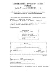
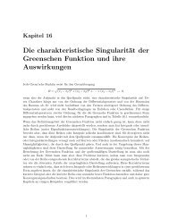
This means, that even at zero temperature the fluctuations will diverge as<br />
the thermodynamic limit is made since the sum over all discrete k states<br />
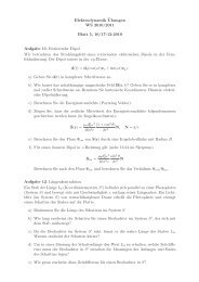
becomes a integral which diverges. This behavior is illustrated in figure 3.1.<br />
That this happens is not surprising since BEC can only take place in systems<br />
with more than one dimension. To be precise it occurs in the two dimensional<br />
case if the gas is trapped or in the free case just at zero temperature. For<br />
three dimensions BEC can take place also for a free gas for higher tempera-<br />
tures than zero [3].<br />
27<br />
1<br />
|k|
Expectation Value of Fluctuation<br />
2.8<br />
2.6<br />
2.4<br />
2.2<br />
2<br />
1.8<br />
1.6<br />
1.4<br />
1.2<br />
1<br />
0.8<br />
0 100 200 300 400 500<br />
L<br />
600 700 800 900 1000<br />
Figure 3.1: Expectation value of the fluctuation ˆ† b R=0 ˆ <br />
bR=0 for different<br />
values of L. The model parameter were set to: t = U = 1 and n = N = 10. L<br />
As expected the fluctuation diverges logarithmically with growing L.<br />
3.2 Particles in a Harmonic Potential<br />
In that case a potential V (R) = α(R − L<br />
2 )2 , with arbitrary constant α, was<br />
used. Again the expectation value of the number operator can be calculated<br />
as:<br />
〈 ˆ ψ †<br />
R ˆ ψR〉 = |φ(R)| 2 + 〈 ˆ b †<br />
R ˆ bR〉 . (3.3)<br />
φ(R) is determined by the Gross-Pitaevskii equation:<br />
28
(V (R) − µ) + U|φ(R)| 2 <br />
) φ(R) − t(φ(R + 1) + φ(R − 1)) = 0 .<br />
This equation has ot be solved numerically, because the particle interac-<br />
tion term U|φ(R)| 2 makes an analytical approach impossible. Finding the<br />
solutions can be done using an iteration, where we start with a certain φ0<br />
calculate with that the particle interaction term U|φ(R)| 2 . After doing that<br />
a simple eigenvalue equation remains. Then we use the eigenvector to the<br />
smallest eigenvalue µ as the new φ0 and iterate until it converges.<br />
The eigenvalue equation for each iteration step is then given by:<br />
With the hermitian and real matrix:<br />
Mφ = µφ . (3.4)<br />
⎛<br />
V (1) + U|φ0(1)|<br />
⎜<br />
M = ⎜<br />
⎝<br />
2 −t<br />
−t<br />
V (2) + U|φ0(2)|<br />
0 · · · −t<br />
2 .<br />
.<br />
−t<br />
.<br />
· · ·<br />
. ..<br />
0<br />
.<br />
−t 0 · · · −t V (L) + U|φ0(L)| 2<br />
⎞<br />
⎟<br />
⎠ .<br />
(3.5)<br />
However this procedure is not very stable and just gives results for a very<br />
limited range of parameters U, t and N0. Because of this I decided to use<br />
another approach. The normalization of the condensate amplitude is:<br />
N0 − <br />
|φ(R)| 2 = 0 (3.6)<br />
R<br />
Together with the GPE this can be considered as a L+1 dimensional function<br />
F (y) from which we want to know the zeros. y is a L+1 dimensional vector<br />
with φ(1), ...φ(L) as the first L entries and with the chemical potential µ as<br />
the last.<br />
The zeros of this function can be easily found using the Newton algorithm:<br />
29
with J the jacobi matrix of F .<br />
yn+1 = yn − (J(yn)) −1 F (yn) , (3.7)<br />
This procedure works pretty well. However we have to make sure that we<br />
truly find a state where the energy is minimal. The left hand side of the<br />
dE GPE is . If the jacobi matrix<br />
dφ(R)<br />
J(R, R ′ ) =<br />
d 2 E<br />
dφ(R) dφ(R ′ )<br />
is positive definite (all eigenvalues are positive for hermitic matrices), φ(R)<br />
is a local minimum. Note that the jacobi matrix J(R, R ′ ) is except the last<br />
row and column 1 the same as the one that was used in the Newton algorithm<br />
3.7.<br />
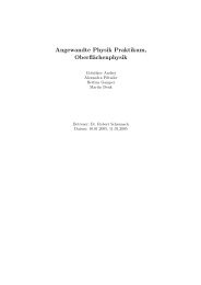
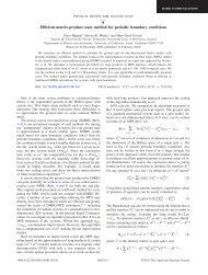
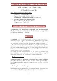
In figures 3.2, 3.3 and 3.4 the results of the Newton algorithm for different<br />
values of the hopping strength t, the interaction strength U and the number<br />
of particles in the ground statetN0 can be seen. As expected higher values<br />
of these parameters cause the particles to spread out more over the whole<br />
lattice, although their potential energy 2 increases.<br />
1 The last row in the Jacobi matrix used in the Newton algorithm came from the<br />
normalization 3.6. The last column from the derivations of the GPE regarding the chemical<br />
potential.<br />
2 In this case I mean with potential energy just the contribution of the external potential<br />
V(R), although the energy from the interaction term U|φ(R)| 2 would also count as<br />
potential energy.<br />
30
|φ (R)|<br />
4.5<br />
4<br />
3.5<br />
3<br />
2.5<br />
2<br />
1.5<br />
1<br />
0.5<br />
0<br />
t=1<br />
t=10<br />
t=100<br />
t=500<br />
5 10 15<br />
R<br />
20 25 30<br />
Figure 3.2: |φ(R)| as a function of the lattice site R for different values of<br />
the hopping strength t. As t increases the particles spread out over the<br />
whole lattice, although they have a higher potential energy at the borders.<br />
The model parameter for the calculation were set to: α = 1, U = 1 and<br />
N0 = 100.<br />
31
|φ (R)|<br />
4.5<br />
4<br />
3.5<br />
3<br />
2.5<br />
2<br />
1.5<br />
1<br />
0.5<br />
0<br />
U=1<br />
U=5<br />
U=10<br />
U=20<br />
5 10 15<br />
R<br />
20 25 30<br />
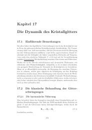
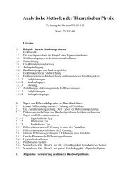
Figure 3.3: |φ(R)| as a function of the lattice site R for different values of<br />
the interaction strength U. Again the particles spread out more the higher<br />
the value of U is chosen. The model parameter for the calculation were set<br />
to: α = 1, t = 1 and N0 = 100.<br />
32
|φ (R)|<br />
4.5<br />
4<br />
3.5<br />
3<br />
2.5<br />
2<br />
1.5<br />
1<br />
0.5<br />
0<br />
N 0 =50<br />
N 0 =100<br />
N 0 =150<br />
N 0 =200<br />
5 10 15<br />
R<br />
20 25 30<br />
Figure 3.4: |φ(R)| as a function of the lattice site R for different values of<br />
number of particles in the ground state N0. Like in the cases before a higher<br />
value of the parameter N0 lets the particles spread out over the whole chain.<br />
On first thought one could assume that the form of the curve should stay the<br />
same, just the hight differs when changing N0. This is because in the GPE<br />
φ(R) contributes quadratically and not just linearly. So instead of increasing<br />
φ(R) at a certain place R much more energy can be saved if the particles<br />
move to the borders. The model parameter for the calculation were set to:<br />
α = 1, t = 10 and U = 5.<br />
To calculate the fluctuations 〈 ˆ b †<br />
R ˆ bR〉 of the mean occupation |φ(R)| 2 , first<br />
the multi-mode Bogoliubov transformation UV has to be constructed. U<br />
consists of the eigenvectors of the matrix SM, with M defined in equation<br />
2.31. This eigenvalue equation arises from the condition of the Hamiltonian<br />
to be diagonal. In addition to this a orthogonal basis from a degenerate<br />
subspace of SM has to be choosen.<br />
33
The matrix V, on the other hand, arises from the second condition on the<br />
transformation: to conserve the bosonic commutation relation (see equation<br />
2.34). V is a diagonal matrix and insures that the commutator of two p-<br />
operators is really 1 and not just a number, what normally occurs in the<br />
numeric calculations. Furthermore the order of the eigenvectors has to be<br />
changed since S is strictly defined with diagonal elements +1 for the first L<br />
indices and −1 for the other half.<br />
With that it is known how the operators B transforms into the operators<br />
P . From the latter the expectation value (equation 1.1) is known, since the<br />
Hamiltonian is diagonal in them.<br />
Since all the above mentioned procedures are pretty time consuming to pro-<br />
gram I decided not to calculate any of the properties and stop at the point<br />
where I have calculated the energies and the Multi-Mode Bogoliubov trans-<br />
formation.<br />
34
Appendix A<br />
Substituting the Bogoliubuv<br />
approximation into the<br />
Hamiltonian<br />
Starting from the Hamiltonian:<br />
H = <br />
(V (R) − µ) ˆ ψ †<br />
R<br />
R ˆ ψR<br />
<br />
H1<br />
and substituting:<br />
− t <br />
leads for the first term called H1 to:<br />
H1 = <br />
R<br />
R<br />
ˆψ †<br />
R ˆ ψR+1 + ˆ ψR ˆ ψ †<br />
R+1<br />
<br />
H2<br />
ˆψR = φ(R) + ˆ bR ,<br />
(V (R) − µ)(|φ(R)| 2 + φ(R) ˆb †<br />
R + φ(R)ˆbR + ˆb †<br />
35<br />
+ U <br />
2<br />
R<br />
<br />
H3<br />
<br />
( ˆ ψ †<br />
R )2 ( ˆ ψR) 2<br />
R ˆ bR) ,<br />
,
equally the next term of the Hamiltonian H2 is given by:<br />
H2 = −t <br />
2φ(R)φ(R + 1) + ˆbR+1φ(R) + ˆbRφ(R + 1)+<br />
R<br />
ˆ b †<br />
R+1 φ(R) + ˆ b †<br />
R φ(R + 1) + ˆ b †<br />
R ˆ bR+1 + ˆ bR ˆ b †<br />
R+1 .<br />
With an index transformation R + 1 = R ′ and using the periodic boundary<br />
conditions in the terms linear in ˆ bR+1 and ˆ b †<br />
R+1 , H2 can be written as:<br />
H2 = −t <br />
2φ(R)φ(R + 1) + ˆbRφ(R − 1) + ˆbRφ(R + 1)+<br />
R<br />
ˆ b †<br />
R φ(R − 1) + ˆ b †<br />
R φ(R + 1) + ˆ b †<br />
R ˆ bR+1 + ˆ bR ˆ b †<br />
R+1 .<br />
Similar calculation for the last term H3:<br />
H3 = U<br />
2<br />
<br />
R<br />
φ(R) 4 + 2 ˆ bRφ(R) 2 φ(R) + 2 ˆ b †<br />
R φ(R)2 φ(R)+<br />
ˆ b 2 Rφ(R) 2 + ˆ (b †<br />
R )2 φ(R) 2 + 4|φ(R)| 2ˆ b †<br />
R bR+<br />
2(b †<br />
R )2ˆ bRφ(R) + 2 ˆ b †<br />
R b2 Rφ(R) + (b †<br />
R )2ˆ b 2 R .<br />
Adding those three parts together and collecting terms like exponents in the<br />
fluctuation operators results in equation 2.5.<br />
36
Appendix B<br />
Performing the Fourier<br />
transformation for the free<br />
particles<br />
Starting point is the Hamiltonian:<br />
H =C + <br />
R<br />
A ˆ b †<br />
R ˆ bR<br />
<br />
H1<br />
+ B( ˆb 2 R + ˆ (b †<br />
R )2 )<br />
<br />
H2<br />
<br />
−t ˆ† b R ˆbR+1 + ˆbR ˆb †<br />
<br />
R+1<br />
<br />
H3<br />
A Fourrier transformation given in equations 2.13 is performed. Again the<br />
Hamiltonian is split up into 3 parts. For the first term called H1:<br />
H1 = <br />
R<br />
A 1<br />
L<br />
= <br />
Aˆb †<br />
k,k ′<br />
= <br />
k,k ′<br />
<br />
k,k ′<br />
k ′ˆ bk<br />
e i(k−k′ )Rˆ b †<br />
k ′ˆ bk<br />
1 <br />
L<br />
A ˆ b †<br />
k ′ˆ bkδk,k<br />
37<br />
R<br />
e i(k−k′ )R<br />
′ = <br />
k<br />
A ˆ b †<br />
k ˆ bk .<br />
.<br />
(B.1)
Where a representation of the delta distribution (the Kronecker delta in<br />
1<br />
that case) δk,k ′ = L<br />
<br />
R ei(k−k′ )R was used in the second line.<br />
Fourier transforming the second term leads to:<br />
H2 = B <br />
R<br />
= B <br />
k,k ′<br />
ˆ b 2 R + ( ˆ b †<br />
R )2<br />
1<br />
N<br />
<br />
R<br />
= B <br />
( ˆbk ˆbk ′ + ˆb †<br />
k,k ′<br />
= B <br />
Finally the last term becomes:<br />
k<br />
H3 = −t <br />
R<br />
= −t <br />
k,k ′<br />
= −t <br />
k<br />
e i(k′ +k)Rˆ bk ˆ bk ′ + e−i(k′ +k)Rˆ b †<br />
k ˆ b †<br />
k ′<br />
k ˆb †<br />
k ′)δk,−k ′<br />
ˆ bk ˆ b−k + ˆ b †<br />
k ˆ b †<br />
−k<br />
ˆ b †<br />
R ˆ bR+1 + ˆ bR ˆ b †<br />
R+1<br />
(e ik′ ˆ b †<br />
k ˆbk ′ + e−ikˆbk ˆb † 1 <br />
k ′)<br />
N<br />
e ikˆ b †<br />
k ˆ bk + e −ik (1 + ˆ b †<br />
k ˆ bk)<br />
= −t <br />
e ik − 2t <br />
k<br />
k<br />
ˆ b †<br />
k ˆ bk cos k<br />
e i(k−k′ )R<br />
<br />
R<br />
<br />
δk,k ′<br />
<br />
Where in the third line the bosonic commutation relations were used. That<br />
the set operators ˆ bk and ˆ b †<br />
k<br />
really obey them is shown in Appendix C.<br />
38
Appendix C<br />
Proof of conservation of<br />
bosonic- commutation relation<br />
The proof will be done for an expansion of operators ˆbR and ˆb †<br />
R in an arbitrary<br />
set of orthonormal functions ψk(R) with operators ˆbk and ˆb †<br />
k :<br />
ˆbR = <br />
ψk(R) ˆbk ˆ b †<br />
R<br />
k<br />
= <br />
k<br />
ψ ∗ k(R) ˆ b †<br />
k<br />
(C.1)<br />
Multiplying the first line with ψ∗ k ′ and the second one with ψk ′ and summing<br />
over all R leads to:<br />
<br />
R<br />
<br />
R<br />
ˆ bR ψ ∗ k<br />
ˆ b †<br />
R<br />
<br />
′(R) = ˆbk ψk(R)ψ ∗ k ′(R) = ˆbk ′<br />
k<br />
ψk ′(R) = <br />
k<br />
ˆ b †<br />
k<br />
R<br />
<br />
ψ ∗ k(R)ψk ′(R)<br />
R<br />
<br />
δk,k ′<br />
<br />
39<br />
= ˆ b †<br />
k ′<br />
(C.2)
Calculation now the commutator [ ˆ bk, ˆ b †<br />
k ]:<br />
[ ˆbk, ˆb †<br />
k ′] = <br />
R,R ′<br />
ψ ∗ k(R)ψk ′(R′ ) [ ˆ bR, ˆ b †<br />
R ′]<br />
<br />
δ R,R ′<br />
= <br />
R<br />
ψ ∗ k(R)ψk ′(R) = δk,k ′ . (C.3)<br />
That the commutators [ ˆb †<br />
k , ˆb †<br />
k ′] and [ ˆbk, ˆbk ′] vanish is trivial.<br />
Hence it has been proven, that if the set of operators ˆbR and ˆb †<br />
R<br />
commutation relation so do the operators ˆ bk and ˆ b †<br />
k .<br />
40<br />
obey the
Appendix D<br />
Calculating the 2L × 2L matrix<br />
for the multi-mode Bogoliubov<br />
transformation<br />
The goal is to find a matrix M which fulfills:<br />
B † M B = <br />
R<br />
<br />
ζ(R)( ˆb †<br />
R ˆbR+ ˆbR ˆb †<br />
R )+η(R)<br />
<br />
ˆ2 bR+ ˆ (b †<br />
R )2<br />
<br />
−¯t ˆ† b R ˆbR+1+ ˆbR+1 ˆb †<br />
R +ˆbR ˆb †<br />
R+1 +ˆb †<br />
R+1 ˆ <br />
bR .<br />
The product B † MB can be rewritten as:<br />
41<br />
(D.1)
B † M B =<br />
=<br />
<br />
L<br />
Mmkbk +<br />
2L<br />
B<br />
m=1<br />
† 2L<br />
2L<br />
m MmnBn = B<br />
n=1<br />
m=1<br />
† m<br />
k=1<br />
L L<br />
Mikb<br />
i=1 k=1<br />
†<br />
ibk L<br />
+<br />
2L<br />
Milb<br />
i=1 l=L+1<br />
†<br />
ib† l +<br />
2L L<br />
Mjkbjbk +<br />
2L<br />
2L<br />
Mjlbjb<br />
j=L+1 k=1<br />
j=L+1 l=L+1<br />
†<br />
l<br />
2L<br />
l=L+1<br />
Mmlb †<br />
<br />
l<br />
(D.2)<br />
Because the multiplication of a Matrix with a vector is linear it is usefull<br />
to split the sum into three terms and calculate the Matrix Mi for each of<br />
them individually.<br />
The first term of D.1 leads to:<br />
B † M1 B ! = <br />
R<br />
ζ(R)( ˆb †<br />
R ˆbR + ˆbR ˆb †<br />
R ) . (D.3)<br />
With the last line of equation D.2 it can be seen, that M1 has to fulfill:<br />
⎧<br />
⎪⎨<br />
ζ(i) · δi,j , ∀ i, j ∈ [1, L]<br />
M1,ij = ζ(i − L) · δi,j ,<br />
⎪⎩<br />
0 , else<br />
∀ i, j ∈ [L + 1, 2L]<br />
The matrix M2 has to satisfy:<br />
B † M2 B = <br />
R<br />
<br />
η(R) ˆ2 bR + ˆ (b †<br />
R )2<br />
<br />
42<br />
(D.4)<br />
(D.5)
Equating coefficients from D.2 gives the matrix M2:<br />
⎧<br />
⎪⎨<br />
η(i) · δi+L,j , ∀ i ∈ [1, L] , j ∈ [L + 1, 2L]<br />
M2,ij = η(i) · δi,j+L , ∀ i ∈ [L + 1, 2L] , j ∈ [1, L]<br />
⎪⎩<br />
0 , else<br />
M3 finally has to fulfill:<br />
so that:<br />
B † M3 B = <br />
R<br />
(D.6)<br />
<br />
−¯t ˆ† b R ˆbR+1 + ˆbR+1 ˆb †<br />
R + ˆbR ˆb †<br />
R+1 + ˆb †<br />
R+1 ˆ <br />
bR , (D.7)<br />
⎧<br />
−¯t · δi+1,j ∀ i ∈ [1, L − 1]<br />
−¯t · δi,j+1 ∀ j ∈ [1, L − 1]<br />
−¯t · δi+1,j ∀ i ∈ [L + 1, 2L − 1]<br />
⎪⎨<br />
−¯t · δi,j+1 ∀ j ∈ [L + 1, 2L − 1]<br />
M3,ij = −¯t for i = L and j = 1<br />
−¯t for i = 1 and j = L<br />
−¯t for i = 2L and j = L<br />
−¯t for i = L and j = 2L<br />
⎪⎩ 0 , else<br />
(D.8)<br />
This complicated expression means, that if M3 is divided into four sectors,<br />
like it is done in 2.31, it is an matrix with the element −¯t above and under<br />
the main diagonal of the upper left and lower right sector. In addition to<br />
this there are four extra entries at the corners of these sectors because of the<br />
periodic boundary condition.<br />
The whole matrix M is then simply given by the sum of all of these 3<br />
matrices, what proofs 2.31.<br />
43
Appendix E<br />
Derivation of the condition for<br />
the commutation relations for<br />
the multi-mode Bogoliubov<br />
transformation<br />
The goal to derivate that if B = U P then:<br />
[ B, B † ] = U[ P , P † ]U † , (E.1)<br />
will be achieved in matrix notation. Therefore it is important first to de-<br />
fine what actually the commutator of two vectors is. The simple expression<br />
[ B, B † ] = B B † − B † B is in fact not even defined, since the B B † is a matrix<br />
of operators and B † B is a scalar operator. 1<br />
Because the commutator just makes sense for single elements of these vectors<br />
1 B is a column vector and B † a row vector.<br />
44
like in 2.32 we can see that:<br />
[ B, B † ] = B B † −<br />
<br />
( B † ) T ( B) T<br />
†<br />
(E.2)<br />
leads to the desired matrix S. Unlike in matrices with scalar entries it’s not<br />
allowed to simplify ( B † ) T ( B) T to ( B B † ) T , because the operators doesn’t com-<br />
mute. This can be recognized by just looking on the first diagonal entries of<br />
both expressions.<br />
With the commutator defined it is possible to plug in the multi mode Bo-<br />
goliubov transformation B = U P :<br />
[ B, B † ] = U P P † U † −<br />
= U P P † U † −<br />
<br />
( P † U † ) T (U P ) T<br />
†<br />
<br />
(U † ) T<br />
†<br />
† T<br />
(P ) P T T<br />
U<br />
= U P P † U † − (U T ) †<br />
<br />
( P † ) T ( P ) T<br />
†<br />
U T<br />
= U[ P , P † ]U †<br />
The last line is only correct if U is assumed to be a real transformation (all<br />
entries are real).<br />
Note that in the second line instead of ( P † U † ) T the expression (U † ) T (P † ) T<br />
can be written, because the multiplication of an operator from P † with a<br />
scalar element of U commutes.<br />
45
Bibliography<br />
[1] Michael Knap, Enrico Arrigoni, and Wolfgang von der Linden. Variational<br />
cluster approach for strongly-correlated lattice bosons in the superfluid<br />
phase, October 2010.<br />
[2] Torsten Fließbach. Statistische <strong>Physik</strong> - Lehrbuch zur <strong>Theoretische</strong>n<br />
<strong>Physik</strong> IV, volume 5. Springer Verlag, 2010.<br />
[3] Christopher Gies. Hartree-fock-bogoliubov treatment of the two-<br />
dimensional trapped bose gas. Master’s thesis, University of Otago,<br />
Dunedin, May 2004.<br />
[4] A. J. Leggett. Bose-einstein condensation in the alkali gases: Some fun-<br />
damental concepts. Rev. Mod. Phys., 73:307–356, 2001.<br />
46