Stage Operation Material Balances 1. Simple Mass ... - Courses
Stage Operation Material Balances 1. Simple Mass ... - Courses
Stage Operation Material Balances 1. Simple Mass ... - Courses

You also want an ePaper? Increase the reach of your titles
YUMPU automatically turns print PDFs into web optimized ePapers that Google loves.
◊ <strong>Stage</strong> <strong>Operation</strong> <strong>Material</strong> <strong>Balances</strong><br />
<strong>1.</strong> <strong>Simple</strong> <strong>Mass</strong> Balance and Units<br />
V 1<br />
L 1<br />
y<br />
1<br />
x 1<br />
x , y<br />
V 2<br />
L 2<br />
y 2<br />
x 2<br />
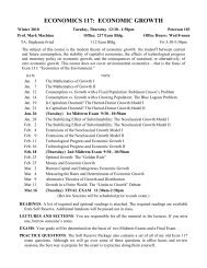
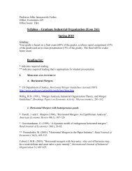
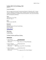
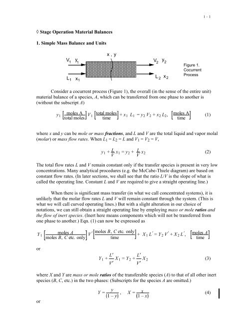
Figure <strong>1.</strong><br />
Cocurrent<br />
Process<br />
Consider a cocurrent process (Figure 1), the overall (in the sense of the entire unit)<br />
material balance of a species, A, which can be transferred from one phase to another is<br />
(without the subscript A)<br />
y1<br />
moles A<br />
total moles<br />
V1 total moles<br />
time<br />
+ x1 L1 = y2 V2 + x2 L2,<br />
moles A<br />
time<br />
where x and y can be mole or mass fractions, and L and V are the total liquid and vapor molal<br />
(molar) or mass flow rates. When L1 = L2 = L and V1 = V2 = V,<br />
y1 + L V x1 = y2 + L V x2<br />
The total flow rates L and V remain constant only if the transfer species is present in very low<br />
concentrations. Many analytical procedures (e.g. the McCabe-Thiele diagram) are based on<br />
constant flow rates. (In later sections, we shall see that the ratio L/V is the slope of what is<br />
called the operating line. Constant L and V are required to give a straight operating line.)<br />
When there is significant mass transfer (in what we call concentrated systems), it is<br />
unlikely that the molar flow rates L and V will remain constant through the system. (This is<br />
what we will call curved operating lines.) But with a slight alteration in our choice of<br />
notations, we can still obtain a straight operating line by employing mass or mole ratios and<br />
the flow of inert species. (Inert here means components which will not be transferred from<br />
one phase to another.) Eqn. (1) can now be expressed as<br />
Y 1<br />
or<br />
moles A<br />
moles B, C etc. only<br />
V ′ moles B, C etc. only<br />
time<br />
Y 1 + L′<br />
X 1 = Y 2 +<br />
V′<br />
L′<br />
X 2<br />
V′<br />
+ X 1 L ′ = Y 2 V ′ + X 2 L ′ ,<br />
1 – 1<br />
moles A<br />
time<br />
where X and Y are mass or mole ratios of the transferable species (A) to that of all other inert<br />
species (B, C, etc.) in the two phases: (Subscripts for the species A are omitted.)<br />
or<br />
Y =<br />
y<br />
1 – y , X = x<br />
1 – x<br />
(1)<br />
(2)<br />
(3)<br />
(4)
= Y<br />
1 + Y<br />
, x = X<br />
1 + X<br />
A few redundant notes: V1 is the total flow rate entering stage 1 according to Fig. 1<br />
and y1 is the concentration of A in the stream V<strong>1.</strong> When the concentration is low, eqn. (4)<br />
indicates that Y = y and X = x. <strong>Mass</strong> or mole ratios are very useful in analysis and design of<br />
gas absorption and liquid extraction processes.<br />
Also, the total flow rates in eqn. (1) can be calculated as<br />
V1 = V′<br />
1 – y1<br />
, L1 =<br />
L′<br />
1 – x1<br />
, etc.<br />
The mass or molar flow rates of the inert species are denoted by L′ and V′ and they remain<br />
constant through the process no matter how many moles of A are being transferred between<br />
the two phases. (The simplest scenario is a binary mixture in either phase such that L′ and V′<br />
are just pure solvent flow rates, and X and Y are mole ratios of the solute A to the solvents in<br />
either phase.)<br />
For ease of typing, all material balances below are only in terms of mass or mole<br />
fractions, and in the form of constant total flow rates. You should change the notations<br />
accordingly to mass or mole ratios when you know that constant total flow rates may not<br />
apply.<br />
That is, you make the decision on the choice of x or X. For dilute systems, the<br />
mathematics is really the same. We just change the notations from x to X, L to L′, etc. For<br />
concentrated systems, you know that the use of mole fractions will not give you a linear<br />
operating line. If we are using a computer, it does not really matter. We will do very well<br />
with x no matter what. Remember that most of these methods in this class were developed in<br />
the slide-rule age and we are aiming toward developing simple (but actually rather ingenious)<br />
graphical solutions to our mass balances.<br />
In the following equations, the notation we used is common to gas-liquid operations.<br />
The gas flow rate and concentration are V and y and the corresponding variables for the<br />
liquid phase are L and x.<br />
1 – 2
2. Cocurrent Processes<br />
Consider again the cocurrent process in Figure <strong>1.</strong> Eqn. (1) is the overall material<br />
balance. We rewrite eqn. (2), with L and V constant, to represent in general the<br />
concentrations of the two streams at any point within the process (the black box) as related to<br />
the inlet:<br />
or<br />
L<br />
V (x1 – x) = y – y1<br />
y = – L V x + y1 + L V x1<br />
This relation is referred to as the operating line and has a negative slope on a y-x diagram.<br />
(Note that this is different from the equilibrium line which provides the relation between<br />
exiting streams of an equilibrium stage. This will be cleared up later when we have to write<br />
the balance equations of an equilibrium stage process. An equilibrium stage is also called an<br />
ideal or theoretical stage; these terms are interchangeable.)<br />
Question: Where should the operating line lie?<br />
1 – 3<br />
For a transfer of the species A from the L (liquid) to V (gas) phase (stripping),<br />
x2 < x 1 and y 2 > y 1 , and the driving force (x – x*) has to be positive. Hence the<br />
operating line is below the equilibrium line.<br />
For a transfer of the species A from the V to L phase (absorption), y 2 < y 1 and<br />
x 2 > x 1 , and the driving force (y – y*) has to be positive. Hence the operating line<br />
is above the equilibrium line.<br />
Question: What is the form of eqn. (2a) when the process is an equilibrium stage operation?<br />
In this case, y 2 = mx 2 , and equation (2a) is usually rearranged to the form<br />
or<br />
where<br />
x2 = x1 + 1/A x*in<br />
1 + (1/A)<br />
, x*in = y1<br />
m<br />
(2a)<br />
Stripping (5a)<br />
y2 = y1 + Ay*in , y*in = mx1 Absorption (5b)<br />
A = L<br />
mV<br />
is the absorption factor. (As far as nomenclature goes, do not confuse the<br />
absorption factor A with the species A.) The stripping factor, S, is sometimes used<br />
to denote 1/A.
1 – 4<br />
NOTE: In this development, we have assumed that the phase equilibrium can be<br />
described by the simple linear relation y* = mx*. This is usually adequate for gas<br />
absorption operations. We shall consider nonlinear equilibrium lines in later<br />
chapters.<br />
Question: What is the thermodynamic relation which provides the linear equilibrium<br />
relation?<br />
Question: Why is A called the absorption factor? Why are there two different form of<br />
equations for stripping and absorption?<br />
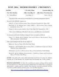
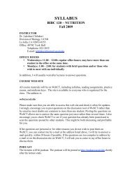
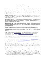
3. Countercurrent Processes<br />
V 1<br />
L 1<br />
y<br />
1<br />
x 1<br />
x , y<br />
The operating line equation for Figure 2, based on the left end, is<br />
or<br />
y = L V x + y1 – L V x1<br />
V2 y<br />
2 Figure 2.<br />
Countercurrent<br />
Process<br />
L 2<br />
x 2<br />
L<br />
V (x1 – x) = y1 – y<br />
When there is a single stage and is in equilibrium, y 1 =mx 2 , the corresponding equations to<br />
Figure 2 are<br />
x2 = x1 + 1/A x*out<br />
1 + 1/A<br />
, x*out = y2<br />
m<br />
y1 = y2 + Ay*out , y*out = mx1<br />
The absorption factor is defined as above. (Note that the subscripts here are very different<br />
from what we shall use later in section 5.)<br />
Question: Show that the operating line for a countercurrent stripping process is below the<br />
equilibrium line, while the operation line of countercurrent absorption is above<br />
the equilibrium line.<br />
Question: Sketch the y and y * profiles for both cocurrent and countercurrent equilibrium<br />
multistage processes.<br />
Question: If the liquid and gas inlet concentrations and the gas outlet concentration are<br />
specified, what is the minimum liquid flow rate (or minimum operating line slope)?<br />
(6)<br />
(7a)<br />
(7b)
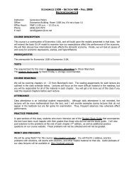
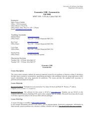
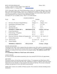
4. Cross-Flow Cascades<br />
L<br />
x<br />
o<br />
V, y V, y V, y<br />
L<br />
1 i–1 i<br />
i+1<br />
xi–1 i<br />
V, y o<br />
i–1<br />
1 – 5<br />
L L<br />
V, y V, y V, y<br />
o o o<br />
Figure 3. Cross-flow Process<br />
The material balance of the transfer species of stage i in Figure 3 is<br />
or<br />
Lxi–1 + Vyo = Lxi + Vyi<br />
yi = – L V xi + yo + L V xi-1<br />
i<br />
i+1<br />
x x<br />
where V is now the gas flow rate to each individual stage. If the stage reaches phase<br />
equilibrium, y i = mx i , and<br />
xi = xi-1 + 1/A x*in<br />
1 + 1/A<br />
, x*in = yo<br />
m<br />
yi = yo + Ay*in , y*in = mxi-1<br />
Question: Sketch the operating lines for stripping and absorption processes.<br />
Question: Sketch the operating lines for a cross-flow cascade with equilibrium stages.<br />
Question: Repeat with non-equilibrium stages.<br />
Question: Compare the separation "efficiency" of cocurrent, countercurrent and<br />
crosscurrent processes. Why is countercurrent processes more effective?<br />
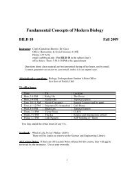
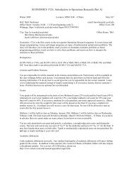
5. Kremser, Souders and Brown (KSB) Equation<br />
In unit operation design calculations, it is useful to find out the quality of separation<br />
for a given number of stages. It is also useful to find the required number of stages if the<br />
product recovery is specified. The development was first given by Kremser in 1930, and by<br />
Souders and Brown in 1932. The resulting equations are referred to as the KSB or Kremser<br />
equations.<br />
Consider a countercurrent process with equilibrium stages (Figure 4). We define<br />
i+1<br />
(8)<br />
(9a)<br />
(9b)
the absorption factorA = L<br />
mV ,<br />
or the stripping factor S = mV<br />
L<br />
and<br />
For stage 1:<br />
or<br />
= 1<br />
A<br />
x * out = yAo m = yAin m<br />
xA1 + VyA1 = LxA2 + VyAo , yA1 = mxA1<br />
xA2 – xA1 = S xA1 – x*out<br />
The material balance over stage 2 and the bottom:<br />
or<br />
Now subtract eqn. (10) from (11):<br />
xA1 + VyA2 = LxA3 + VyAo<br />
xA3 – xA1 = S xA2 – x*out<br />
xA3 – xA2 = S xA2 – xA1<br />
1 – 6<br />
(10)<br />
(11)<br />
(11a)<br />
(Note that this is a clumsy way to get eqn. (11a). This equation is nothing but the material<br />
balance of stage 2 in equilibrium. The derivation is just to show that there are more ways<br />
than one to do things, but we are dealing with simple mass balances and the result has to be<br />
the same.)<br />
Substitute eqn. (10) in (11a):<br />
xA3 – xA2<br />
xA1 – x *<br />
out<br />
Now try this one more time with stage number 3. We should get<br />
and<br />
With similar procedures, for any stage i,<br />
x A4 – x A1 = S (x A3 – x * out )<br />
x A4 – x A3 = S (x A3 – x A2 )<br />
xi+1 – xi<br />
xA1 – x *<br />
out<br />
Now add up all the balances of stages 1 to n:<br />
= S 2 (11b)<br />
= (xA1 – x * out ) S3<br />
= S i (12)
xAn+1 – xA1<br />
xA1 – x *<br />
out<br />
n<br />
∑<br />
= S k<br />
We can rearrange eqn. (13) by adding and subtracting the term xAn+1∑Sk and writing<br />
xAn+1 = xAin and xA1 = xAout :<br />
The final result is<br />
xAin – xAout<br />
xAin – x *<br />
out<br />
xAin – xAout<br />
xAin – x *<br />
k=1<br />
n<br />
∑<br />
k=1<br />
S k<br />
=<br />
1 + S k<br />
n<br />
=<br />
n<br />
∑<br />
k=0<br />
∑ n<br />
∑<br />
k=1<br />
S k<br />
S k<br />
– 1<br />
= S – S n+1<br />
1 – S n+1<br />
Equation (14) can further be rearranged to the forms<br />
and<br />
n =<br />
xAout – x *<br />
Aout<br />
xAin – x *<br />
= 1 – S<br />
1 – S n+1<br />
ln 1–A xAin - x *<br />
Aout<br />
xAout - x *<br />
Aout<br />
ln [S]<br />
+ A<br />
1 – 7<br />
(13)<br />
(13a)<br />
(14)<br />
(14a)<br />
(14b)<br />
The entire derivation can be carried out turning the procedure upside down, i.e., starting with<br />
stage N and the material balances in terms of y. The corresponding equations to eqns. (10)<br />
and (11b) are eqns. (15a) and (15b).<br />
For stage N:<br />
and stage N–1:<br />
yAn-1 – yAn<br />
yAn – y*out<br />
= A , y*out = mxAin<br />
yAn-2 – yAn-1<br />
yAn – y*out<br />
The corresponding form of eqn. (12) for any stage i is<br />
Sum up all the stages:<br />
yAi – yAi+1<br />
yAn – y*out<br />
(15a)<br />
= A 2 (15b)<br />
= A n–i (16)
yAo – yAn<br />
An – y*out<br />
n<br />
∑<br />
= A n<br />
The final results corresponding to eqns. (14), (14a) and (14b) are<br />
and<br />
n =<br />
yAin – yAout<br />
yAin – y*out<br />
yAout – y*out<br />
yAin – y*out<br />
= A – A n+1<br />
= 1 – A<br />
k=1<br />
1 – A n+1<br />
1 – A n+1<br />
1n 1–S yAin - y *<br />
out<br />
yAout - y *<br />
out<br />
ln [A]<br />
+ S<br />
1 – 8<br />
(17)<br />
(17a)<br />
(17b)<br />
Note that eqns. (14) and (17) are very similar (and mathematically identical). All you have to<br />
do is interchange x and y, S and A.<br />
Question: When you solve either a stripping or an absorption problem, does it matter<br />
whether you use eqn. (14) or (17)?<br />
Question: Derive the corresponding form of the Kremser equation for the cross-flow<br />
cascade. Show that when yo=0, how the equation simplifies. (The answer is<br />
below, but try to do it yourself first.)<br />
Question: What about a similar analysis for a cocurrent multistage process?<br />
6. Kremser Equation for Cross-Flow Cascade<br />
Refer back to Fig. 3. The derivation will continue onto stage N on the right. Derive in<br />
terms of X (i.e. stripping), and define<br />
and<br />
<strong>Stage</strong> N:<br />
<strong>Stage</strong> N–1:<br />
S = 1<br />
A<br />
= V′m<br />
L′<br />
X* = Yo<br />
m<br />
V′Y o + L′X N-1 = V′Y N + L′X N , Y N = mX N<br />
X N-1 + S Y o = SXN + X N<br />
X N-1 = X N 1+S – SX* (18)<br />
X N-1 – X N = S X N – X * (18a)
Subtract eqn. (18) from (19):<br />
Substitute eqn. (18a) in (19a):<br />
Now for stage N–2:<br />
Subtract eqn. (19) from (20):<br />
Substitute eqn. (19a) in (20a):<br />
By induction,<br />
Sum up the (b) form of all the stages:<br />
This leads to<br />
′Y o + L′X N-2 = V′Y N-1 + L′X N-1<br />
S Y o<br />
m + X N-2 = SXN-1 + X N-1<br />
1 – 9<br />
X N-2 = X N-1 (1+S) – SX* (19)<br />
X N-2 – X N-1 = X N-1 – X N 1+S (19a)<br />
X N-2 – X N-1 = X N – X * 1+S S (19b)<br />
′Y o + L′X N-3 = V′Y N-2 + L′X N-2<br />
X N-3 = X N-2 1+S – SX* (20)<br />
X N-3 – X N-2 = X N-2 – X N-1 1 + S (20a)<br />
X N-3 – X N-2 = X N – X * 1 + S 2 S (20b)<br />
X o – X 1<br />
X N – X * = S 1 + S N-1 (20c)<br />
X o – X N<br />
X N – X *<br />
N-1<br />
= S + S ∑ (1 + S)k<br />
(21)<br />
S 1 + 1 + S k<br />
N–1<br />
∑<br />
= S 1+S k<br />
N–1<br />
Σk=0<br />
= S<br />
1 – 1 + S N<br />
– S<br />
S 1 + S N – 1
or<br />
When Y o = 0, X * = 0, and<br />
or<br />
1 – 10<br />
X o – X *<br />
X N – X * = 1 + S N (22)<br />
N =<br />
ln X o – X *<br />
X N – X *<br />
ln 1 + S<br />
N =<br />
ln X o<br />
X N<br />
ln 1 + S<br />
X N = 1 + S<br />
X o<br />
–N<br />
This is one of many ways to derive the equation. Try to derive the results a different way. Try<br />
to use x, L, etc.<br />
(23)<br />
(24)