An Assessment of Coupled Inductor Modeling for a Multiâoutput ...
An Assessment of Coupled Inductor Modeling for a Multiâoutput ...
An Assessment of Coupled Inductor Modeling for a Multiâoutput ...

You also want an ePaper? Increase the reach of your titles
YUMPU automatically turns print PDFs into web optimized ePapers that Google loves.
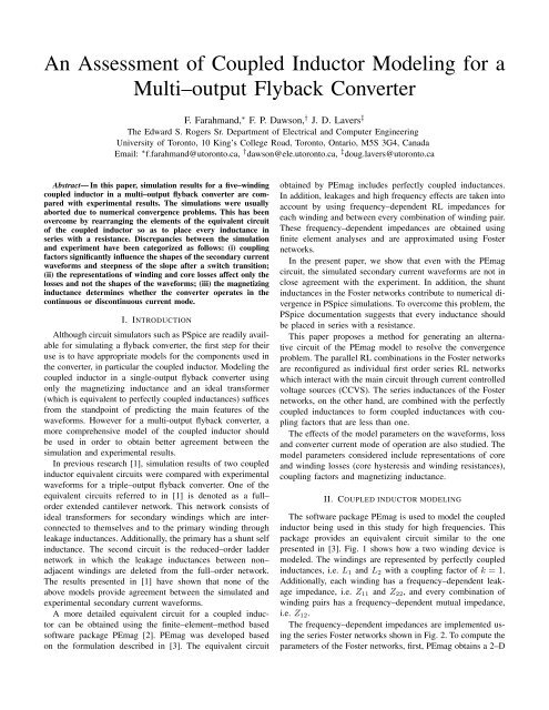
<strong>An</strong> <strong>Assessment</strong> <strong>of</strong> <strong>Coupled</strong> <strong>Inductor</strong> <strong>Modeling</strong> <strong>for</strong> a<br />
Multi–output Flyback Converter<br />
F. Farahmand, ∗ F. P. Dawson, † J. D. Lavers ‡<br />
The Edward S. Rogers Sr. Department <strong>of</strong> Electrical and Computer Engineering<br />
University <strong>of</strong> Toronto, 10 King’s College Road, Toronto, Ontario, M5S 3G4, Canada<br />
Email: ∗ f.farahmand@utoronto.ca, † dawson@ele.utoronto.ca, ‡ doug.lavers@utoronto.ca<br />
Abstract— In this paper, simulation results <strong>for</strong> a five–winding<br />
coupled inductor in a multi–output flyback converter are compared<br />
with experimental results. The simulations were usually<br />
aborted due to numerical convergence problems. This has been<br />
overcome by rearranging the elements <strong>of</strong> the equivalent circuit<br />
<strong>of</strong> the coupled inductor so as to place every inductance in<br />
series with a resistance. Discrepancies between the simulation<br />
and experiment have been categorized as follows: (i) coupling<br />
factors significantly influence the shapes <strong>of</strong> the secondary current<br />
wave<strong>for</strong>ms and steepness <strong>of</strong> the slope after a switch transition;<br />
(ii) the representations <strong>of</strong> winding and core losses affect only the<br />
losses and not the shapes <strong>of</strong> the wave<strong>for</strong>ms; (iii) the magnetizing<br />
inductance determines whether the converter operates in the<br />
continuous or discontinuous current mode.<br />
I. INTRODUCTION<br />
Although circuit simulators such as PSpice are readily available<br />
<strong>for</strong> simulating a flyback converter, the first step <strong>for</strong> their<br />
use is to have appropriate models <strong>for</strong> the components used in<br />
the converter, in particular the coupled inductor. <strong>Modeling</strong> the<br />
coupled inductor in a single-output flyback converter using<br />
only the magnetizing inductance and an ideal trans<strong>for</strong>mer<br />
(which is equivalent to perfectly coupled inductances) suffices<br />
from the standpoint <strong>of</strong> predicting the main features <strong>of</strong> the<br />
wave<strong>for</strong>ms. However <strong>for</strong> a multi-output flyback converter, a<br />
more comprehensive model <strong>of</strong> the coupled inductor should<br />
be used in order to obtain better agreement between the<br />
simulation and experimental results.<br />
In previous research [1], simulation results <strong>of</strong> two coupled<br />
inductor equivalent circuits were compared with experimental<br />
wave<strong>for</strong>ms <strong>for</strong> a triple–output flyback converter. One <strong>of</strong> the<br />
equivalent circuits referred to in [1] is denoted as a full–<br />
order extended cantilever network. This network consists <strong>of</strong><br />
ideal trans<strong>for</strong>mers <strong>for</strong> secondary windings which are interconnected<br />
to themselves and to the primary winding through<br />
leakage inductances. Additionally, the primary has a shunt self<br />
inductance. The second circuit is the reduced–order ladder<br />
network in which the leakage inductances between non–<br />
adjacent windings are deleted from the full–order network.<br />
The results presented in [1] have shown that none <strong>of</strong> the<br />
above models provide agreement between the simulated and<br />
experimental secondary current wave<strong>for</strong>ms.<br />
A more detailed equivalent circuit <strong>for</strong> a coupled inductor<br />
can be obtained using the finite–element–method based<br />
s<strong>of</strong>tware package PEmag [2]. PEmag was developed based<br />
on the <strong>for</strong>mulation described in [3]. The equivalent circuit<br />
obtained by PEmag includes perfectly coupled inductances.<br />
In addition, leakages and high frequency effects are taken into<br />
account by using frequency–dependent RL impedances <strong>for</strong><br />
each winding and between every combination <strong>of</strong> winding pair.<br />
These frequency–dependent impedances are obtained using<br />
finite element analyses and are approximated using Foster<br />
networks.<br />
In the present paper, we show that even with the PEmag<br />
circuit, the simulated secondary current wave<strong>for</strong>ms are not in<br />
close agreement with the experiment. In addition, the shunt<br />
inductances in the Foster networks contribute to numerical divergence<br />
in PSpice simulations. To overcome this problem, the<br />
PSpice documentation suggests that every inductance should<br />
be placed in series with a resistance.<br />
This paper proposes a method <strong>for</strong> generating an alternative<br />
circuit <strong>of</strong> the PEmag model to resolve the convergence<br />
problem. The parallel RL combinations in the Foster networks<br />
are reconfigured as individual first order series RL networks<br />
which interact with the main circuit through current controlled<br />
voltage sources (CCVS). The series inductances <strong>of</strong> the Foster<br />
networks, on the other hand, are combined with the perfectly<br />
coupled inductances to <strong>for</strong>m coupled inductances with coupling<br />
factors that are less than one.<br />
The effects <strong>of</strong> the model parameters on the wave<strong>for</strong>ms, loss<br />
and converter current mode <strong>of</strong> operation are also studied. The<br />
model parameters considered include representations <strong>of</strong> core<br />
and winding losses (core hysteresis and winding resistances),<br />
coupling factors and magnetizing inductance.<br />
II. COUPLED INDUCTOR MODELING<br />
The s<strong>of</strong>tware package PEmag is used to model the coupled<br />
inductor being used in this study <strong>for</strong> high frequencies. This<br />
package provides an equivalent circuit similar to the one<br />
presented in [3]. Fig. 1 shows how a two winding device is<br />
modeled. The windings are represented by perfectly coupled<br />
inductances, i.e. L1 and L2 with a coupling factor <strong>of</strong> k =1.<br />
Additionally, each winding has a frequency–dependent leakage<br />
impedance, i.e. Z11 and Z22, and every combination <strong>of</strong><br />
winding pairs has a frequency–dependent mutual impedance,<br />
i.e. Z12.<br />
The frequency–dependent impedances are implemented using<br />
the series Foster networks shown in Fig. 2. To compute the<br />
parameters <strong>of</strong> the Foster networks, first, PEmag obtains a 2–D
V1<br />
C 11<br />
Z12 × I2<br />
I1<br />
VT 1<br />
k = 1<br />
L1 L2 Z11 Z22 C 12<br />
C O 12<br />
V T 2<br />
I 2<br />
Z21 × I1<br />
Fig. 1. PEmag equivalent circuit <strong>for</strong> a two winding component<br />
Z 11<br />
i 1<br />
R ser 1<br />
Z 12<br />
i 2<br />
R ser 12<br />
Z21 = Z12 i 1<br />
R ser 12<br />
L ser 1<br />
L ser 12<br />
L ser 12<br />
i par 1<br />
L par 1<br />
R par 1<br />
i 1 −i par 1<br />
i par 12<br />
L par 12<br />
R par 12<br />
i2−ipar<br />
i<br />
par 21<br />
Lpar<br />
12<br />
R par 12<br />
12<br />
1−i i par 21<br />
Z 22<br />
i 2<br />
R ser 2<br />
L ser 2<br />
i par 2<br />
L par 2<br />
R par 2<br />
i−i par<br />
2 2<br />
Fig. 2. PEmag equivalent circuit <strong>for</strong> a two winding component<br />
axisymmetric equivalent representation <strong>of</strong> the magnetic component<br />
[3], if it is 3–D. Then the quasi–static magnetic Finite<br />
Element Method is used to calculate the open circuit frequency<br />
responses <strong>of</strong> the 2–D equivalent magnetic component over a<br />
frequency range that the user has defined. Finally, each Foster<br />
network in Fig. 2 is fitted to the respective frequency response<br />
by minimizing the least means square error.<br />
Capacitive effects between the turns <strong>of</strong> the windings can be<br />
important <strong>for</strong> very high frequencies. To obtain the frequency<br />
responses, PEmag assumes that the displacement currents are<br />
negligible. There<strong>for</strong>e these capacitive effects are ignored. They<br />
are partly compensated using lumped capacitors between the<br />
terminals <strong>of</strong> the windings as illustrated in Fig. 1 [4]. The<br />
lumped capacitors are computed using an electrostatic Finite<br />
Element Method. For the magnetic component studied in this<br />
paper, these capacitors are on the order <strong>of</strong> several pico farads<br />
and <strong>for</strong> our flyback case study, with a 40 kHz switching<br />
frequency, the simulations show no obvious differences in<br />
the wave<strong>for</strong>ms if the capacitances are eliminated from the<br />
equivalent network.<br />
Utilizing a 2–D equivalent magnetic component instead <strong>of</strong><br />
a 3–D component introduces errors in the frequency responses<br />
that are estimated to be no greater than 25% [5]. There are also<br />
errors in fitting the Foster networks to the frequency responses.<br />
In particular, a shortcoming <strong>of</strong> PEmag is that the orders <strong>of</strong> the<br />
Foster networks are fixed and cannot be changed. There<strong>for</strong>e,<br />
V 2<br />
the use <strong>of</strong> a wider range <strong>of</strong> frequency can result in larger errors<br />
when the networks are fitted to the frequency responses. As<br />
an example, the fitting errors <strong>for</strong> our case study increase by<br />
10% from 5–20% to 15–30% when the range <strong>of</strong> frequencies<br />
increases from 0–1 MHz to 0–2 MHz.<br />
The model previously described assumes a linear lossless<br />
core. To include the core loss in the equivalent circuit, one can<br />
consider an equivalent resistance in parallel with L1. However,<br />
the value <strong>of</strong> the resistance is a function <strong>of</strong> operating voltage<br />
and frequency and should be recomputed using approaches<br />
such as those proposed in [6], [7] or [8] if the operating point<br />
changes.<br />
Alternatively, it is possible to include the Jiles–Atherton (J–<br />
A) nonlinear core representation [9] in the circuit. In this way,<br />
PSpice simultaneously incorporates the B–H loop along with<br />
currents and voltages. <strong>An</strong> advantage <strong>of</strong> this method is that<br />
the core loss and impacts <strong>of</strong> a nonlinear core on wave<strong>for</strong>ms<br />
are taken into account inherently. However, numerical convergence<br />
problems are far more severe than the lossless core<br />
model or a model that introduces losses in the <strong>for</strong>m <strong>of</strong> a fixed<br />
resistance.<br />
PSpice simulations using the equivalent circuits given by<br />
PEmag usually exhibit numerical divergence. PSpice produces<br />
error messages that primarily refer to the shunt inductances <strong>of</strong><br />
the Foster networks used in modeling the coupled inductor<br />
as potential sources <strong>of</strong> the convergence problem. The PSpice<br />
documentation recommends that every inductance be placed in<br />
series with a resistance. There<strong>for</strong>e to resolve the convergence<br />
problem, the PEmag network is reconfigured in the <strong>for</strong>m <strong>of</strong><br />
another circuit model which is described next.<br />
A. Alternative network <strong>for</strong> a two winding component<br />
The equivalent network topology shown in Fig. 1 and Fig. 2<br />
is used to show the method <strong>of</strong> extracting the alternative<br />
network from a PEmag circuit. For simplicity, only one parallel<br />
RL branch is taken into account <strong>for</strong> each Foster network in<br />
Fig. 2. Also, no capacitance effects are considered. The results<br />
are extended in the next subsection <strong>for</strong> a general PEmag circuit<br />
with any number <strong>of</strong> windings and parallel branches.<br />
First, Kirchh<strong>of</strong>f’s Voltage Law (KVL) is applied to the<br />
primary side to obtain (1).<br />
v1 = Lser1 ˙i1 + Rser1i1 + Rpar1 (i1 − ipar1 )<br />
+ Lser12 ˙i2 + Rser12i2 + Rpar12 (i2 − ipar12 )<br />
+ vT1<br />
Substituting the coupled inductance characteristic equation, i.e.<br />
(2), into (1) results in (3).<br />
(1)<br />
vT1 = L1 × ˙i1 + � L1L2 × ˙i2<br />
v1 =(L1 + Lser1<br />
(2)<br />
) �� �<br />
˙i1 + L1L2 + Lser12<br />
˙i2<br />
+(Rser1 + Rpar1 ) i1 − Rpar1ipar1 (3)<br />
+(Rser12 + Rpar12 ) i2 − Rpar12 ipar12
v 1<br />
Rpar × i<br />
1 par 1<br />
Rpar × i<br />
12 par 12<br />
i par 1<br />
i1<br />
L par 1<br />
(Rser +R<br />
12 par )× i<br />
12 2<br />
R ser 1 +R par 1<br />
k =<br />
i par 12<br />
L 1 +L ser 1<br />
L par 12<br />
+L ser 2<br />
L 2<br />
L 1 L 2 + L ser 12<br />
(L 1 +L ser 1 )(L 2 +L ser 2 )<br />
R ser +R par<br />
2 2<br />
Rpar × i<br />
12 par 21<br />
(Rser +R )×i<br />
12 par 12 1<br />
L par 12<br />
Rpar × i Rpar × i<br />
12 2<br />
× i<br />
12 1<br />
× i<br />
1 1<br />
Rpar Rpar 2 2<br />
Rpar R R<br />
1<br />
par 12<br />
par 12<br />
i par 21<br />
i2<br />
Rpar × i<br />
2 par 2<br />
i par 2<br />
L par 2<br />
Fig. 3. Alternative circuit <strong>for</strong> Fig. 1 considering only one shunt RL loop <strong>for</strong><br />
the Foster network<br />
Equation (4) is obtained by applying a similar KVL <strong>for</strong> the<br />
secondary side.<br />
v2 =(L2 + Lser2 ) �� �<br />
˙i2 + L1L2 + Lser12<br />
˙i1<br />
+(Rser2 + Rpar2 ) i2 − Rpar2ipar2 (4)<br />
+(Rser12 + Rpar12 ) i2 − Rpar12 ipar21<br />
The KVL’s inside the loops <strong>of</strong> the parallel RL combinations,<br />
i.e. (5), provide governing equations <strong>for</strong> the remaining inductances.<br />
⎧⎪<br />
Lpar1<br />
⎨<br />
⎪⎩<br />
˙ipar1 − Rpar1 (i1 − ipar1 )=0<br />
Lpar12 ˙ipar12 − Rpar12 (i2 − ipar12 )=0<br />
Lpar2 ˙ipar2 − Rpar2 (i2 − ipar2 )=0<br />
Lpar12 ˙ipar21 − Rpar12 (i1 − ipar21 )=0<br />
(5)<br />
Finally, a rearranged <strong>for</strong>mat <strong>of</strong> the above equation, which is<br />
shown in (6), along with (3) and (4) is used to generate the<br />
alternative equivalent network <strong>for</strong> the magnetic component as<br />
shown Fig. 3.<br />
⎧<br />
Lpar1<br />
˙ipar1 + Rpar1ipar1 = Rpar1i1 ⎪⎨<br />
⎪⎩<br />
Lpar12<br />
˙ipar12 + Rpar12ipar12 = Rpar12i2 Lpar2<br />
˙ipar2 + Rpar2ipar2 = Rpar2i2 Lpar12<br />
˙ipar21 + Rpar12ipar21 = Rpar12i1 In summary, with reference to Fig. 3, the series inductances<br />
Lser1 , Lser2 and Lser12 in the Foster networks and the<br />
perfectly coupled inductances L1 and L2 are integrated to <strong>for</strong>m<br />
coupled inductances with a coupling factor that is less than 1.<br />
The shunt inductances in the Foster networks, Lpar1 , Lpar12<br />
and Lpar2 , <strong>for</strong>m separate subnetworks which are linked to the<br />
main circuit by current controlled voltage sources (CCVS).<br />
The transresistance <strong>of</strong> each <strong>of</strong> the CCVS’s equals the shunt<br />
resistance <strong>of</strong> the respective RL loop. For each winding, there is<br />
an additional CCVS which is controlled by the other winding’s<br />
current and has a transresistance that equals the sum <strong>of</strong> all the<br />
resistances in the mutual Foster network Z12. In addition, all <strong>of</strong><br />
the resistances in the impedances Z11 and Z22 appear as series<br />
resistances <strong>for</strong> the primary and secondary circuits respectively.<br />
R par 2<br />
v 2<br />
(6)<br />
i i<br />
Rpar<br />
i i<br />
× ipar<br />
R par<br />
W i<br />
R par<br />
L par<br />
i i−<br />
par i<br />
i par<br />
W i<br />
i par<br />
L par<br />
Rpar<br />
× ii<br />
Rpar<br />
Fig. 4. Alternative network <strong>for</strong> a shunt RL in self impedances<br />
i i<br />
Zpar j<br />
m × I<br />
W i<br />
Rm m<br />
par par Rpar m<br />
ii × i × ij<br />
W i<br />
W j<br />
i j<br />
W j<br />
i j<br />
Rpar m<br />
Lpar m<br />
Rpar m<br />
× ij<br />
Zpar m<br />
Fig. 5. Alternative network <strong>for</strong> a shunt RL in mutual impedances<br />
B. General procedure to generate alternative network<br />
Based on the previous subsection, the following procedure<br />
is proposed to generate the alternative network <strong>for</strong> any PEmag<br />
circuit:<br />
1) Delete all Lser’s and replace every Li <strong>of</strong> the perfectly<br />
coupled inductances with Li + Lseri<br />
2) Change the coupling factor between coupled inductances<br />
i and j from 1 to<br />
kij =<br />
�<br />
�� LiLj + Lserij<br />
ipar m<br />
�<br />
Lpar m<br />
Rpar m<br />
(Li + Lseri ) × � Lj + Lserj<br />
� . (7)<br />
3) Reconfigure each parallel RL branch in the ith self<br />
impedance as shown in Fig. 4. Each RL loop is replaced<br />
with a series resistance and a reversed–polarity CCVS,<br />
and a separate series RL circuit which is supplied by<br />
another CCVS. The transresistances <strong>of</strong> the CCVS’s are<br />
equal to the respective loop’s resistance.<br />
4) Reconfigure each parallel RL branch in the mutual<br />
impedance between windings i and j as shown in Fig. 5.<br />
The procedure is similar to the one shown in Fig. 4 with<br />
the exception that the series resistance is replaced with<br />
another CCVS.<br />
5) Leave all <strong>of</strong> the Rser’s as they are.
C. Alternative network with J–A core representation<br />
For a network that includes a nonlinear J–A core representation,<br />
no coupling factor can be defined using (7) since the<br />
coupled inductances, e.g. L1 and L2, are replaced with the<br />
turn numbers <strong>of</strong> the windings and parameters to define the B–<br />
H loop <strong>of</strong> the core. A method to work around this problem is<br />
to use the coupling factors obtained <strong>for</strong> the linearized network.<br />
However, only one global coupling factor <strong>for</strong> all winding<br />
pairs has to be specified in PSpice if the J–A core model<br />
is used. There<strong>for</strong>e <strong>for</strong> a triple– or higher–winding magnetic<br />
component, items 1 and 2 in the procedure described in<br />
section II-B, should not be considered and only the parallel<br />
RL combinations are reconfigured.<br />
D. Advantages <strong>of</strong> proposed <strong>for</strong>mulation<br />
The alternative circuit results in shorter simulation run times<br />
since the new <strong>for</strong>mulation allows <strong>for</strong> larger time steps. As an<br />
example, <strong>for</strong> our case study, the simulation with the alternative<br />
circuit was about two times faster than that with the PEmag<br />
circuit. Alternatively, solutions can be obtained with better<br />
accuracies using smaller error tolerances. For example <strong>for</strong> our<br />
case study, with respect to the PEmag circuit, the absolute<br />
current error tolerance <strong>for</strong> the alternative circuit simulation<br />
could be lowered by a factor <strong>of</strong> 100 from 10 nA to 0.1 nA<br />
while the simulation run times <strong>for</strong> the original lossless core<br />
circuit and the alternative circuit were approximately the same.<br />
<strong>An</strong> absolute current error tolerance lower than 10 nA resulted<br />
in divergence <strong>for</strong> the simulation with the PEmag circuit.<br />
III. COMPARISON OF SIMULATION AND EXPERIMENTAL<br />
RESULTS<br />
The triple–output flyback converter shown in Fig. 6 has been<br />
studied. The converter has a 14 V output and two 5 V outputs.<br />
One <strong>of</strong> the 5 V outputs is connected to a regulator. The other<br />
5 V output and the 14 V output are connected to a tapped<br />
winding and are controlled by a PWM controller. <strong>An</strong> extra<br />
secondary winding is included in order to power the PWM<br />
controller.<br />
In our experiments, the resistive loads, RL3, RL4 and RL5,<br />
are set such that their measured currents are 500, 700 and 500<br />
mA respectively. The experimental wave<strong>for</strong>ms were logged<br />
in files using a Tektronix TDS3014 oscilloscope. The current<br />
wave<strong>for</strong>ms were obtained using a Tektronix A6312 current<br />
probe. The switching frequency is approximately 40 kHz with<br />
a duty cycle <strong>of</strong> about 14%.<br />
Two equivalent circuits <strong>for</strong> the five–winding coupled inductor<br />
are obtained using PEmag: one with a lossless linear<br />
core and the other one with the J–A model <strong>of</strong> the core. Their<br />
Foster networks are optimized <strong>for</strong> a frequency range from DC<br />
to 1 MHz. The fitting errors range from 5 to 20%. To resolve<br />
convergence problems, the alternative circuits <strong>of</strong> the networks<br />
are used instead <strong>of</strong> the PEmag circuits. We have also simulated<br />
another equivalent circuit in which the core loss is taken into<br />
account using an equivalent shunt resistance. The value <strong>of</strong> the<br />
resistance was calculated to be about 5 kΩ using the primary<br />
voltage wave<strong>for</strong>ms and computed core loss from the equivalent<br />
+<br />
160V<br />
−<br />
Controller<br />
PWM<br />
Current (A)<br />
Current (A)<br />
Current (A)<br />
3<br />
2.5<br />
2<br />
1.5<br />
1<br />
0.5<br />
Q 1<br />
Primary<br />
W1<br />
27 turns<br />
250m<br />
D 2<br />
W2 8 turns<br />
D3 W3 1500µ<br />
4 turns<br />
D4 W4 1500µ<br />
5 turns<br />
W5 3 turns<br />
D 5<br />
6.7V<br />
5V<br />
Regulator<br />
6.8µ<br />
6.8µ<br />
100µ<br />
100µ<br />
1500µ 100µ<br />
Fig. 6. Triple-output flyback converter<br />
144Ω<br />
910Ω<br />
108Ω<br />
5V<br />
500mA<br />
14V<br />
700mA<br />
5V<br />
500mA<br />
Linear Core Model<br />
J−A Core Model<br />
Experiment<br />
0<br />
0 5 10 15 20 25<br />
Time (µs)<br />
30 35 40 45 50<br />
6<br />
5<br />
4<br />
3<br />
2<br />
1<br />
(a) D3 current<br />
0<br />
0 5 10 15 20 25<br />
Time (µs)<br />
30 35 40 45 50<br />
2<br />
1.5<br />
1<br />
0.5<br />
(b) D4 current<br />
0<br />
0 5 10 15 20 25<br />
Time (µs)<br />
30 35 40 45 50<br />
(c) D5 current<br />
Fig. 7. Experimental and simulated current wave<strong>for</strong>ms<br />
circuit with the J–A core model. The simulation shows that the<br />
existence <strong>of</strong> the equivalent shunt resistance does not cause any<br />
visible change to the wave<strong>for</strong>ms with respect to those <strong>of</strong> the<br />
lossless core circuit without the shunt resistance. Hence, no<br />
further study is carried out on this type <strong>of</strong> equivalent circuit.<br />
Fig. 7 compares the simulated and experimental wave<strong>for</strong>ms<br />
<strong>for</strong> the currents <strong>of</strong> the secondary diodes. This figure illustrates<br />
that the equivalent circuits provided by PEmag cannot accurately<br />
replicate the secondary current wave<strong>for</strong>ms. In particular,<br />
there are large differences in the rise times <strong>of</strong> the currents at<br />
a switching transition.<br />
R L3<br />
R L4<br />
RL5
Current (A)<br />
Current (A)<br />
Current (A)<br />
5<br />
4<br />
3<br />
2<br />
1<br />
0<br />
0 5 10 15 20 25<br />
Time (µs)<br />
30 35 40 45 50<br />
(a) Nonlinear (J–A) circuit, Winding loss = 150mW, Core loss = 970mW<br />
5<br />
4<br />
3<br />
2<br />
1<br />
0<br />
0 5 10 15 20 25<br />
Time (µs)<br />
30 35 40 45 50<br />
5<br />
4<br />
3<br />
2<br />
1<br />
(b) Lossless core circuit, Winding loss = 170mW<br />
0<br />
0 5 10 15 20 25<br />
Time (µs)<br />
30 35 40 45 50<br />
(c) Multiplying every resistance by 2, Winding loss = 285mW<br />
IV. EFFECTS OF EQUIVALENT NETWORK PARAMETERS<br />
To understand the reasons <strong>for</strong> the discrepancies between<br />
the simulated and experimental wave<strong>for</strong>ms, the effects <strong>of</strong> the<br />
equivalent circuit parameters on the wave<strong>for</strong>ms are studied and<br />
compared in Fig. 8.<br />
A. Winding and core losses<br />
First <strong>of</strong> all, as Fig. 8(a) and Fig. 8(b) show, the use <strong>of</strong> a<br />
lossless model <strong>for</strong> the core or a J–A core model does not<br />
significantly affect the shapes <strong>of</strong> the simulated wave<strong>for</strong>ms.<br />
However, they have impacts on the total loss. With the linear<br />
lossless core model, the winding loss is estimated to be about<br />
170 mW. The Modified Steinmetz Equation (MSE) method<br />
[7] is used to estimate the core loss from the simulated<br />
magnetizing current. The MSE method is an adaptation <strong>of</strong> the<br />
empirical Steinmetz equation <strong>for</strong> a nonsinusoidal magnetizing<br />
current. The core loss estimate using the MSE method is<br />
on the order <strong>of</strong> 590–685 mW. The network with the J–A<br />
model, on the other hand, predicts a 150 mW winding loss<br />
and a 970 mW core loss. The large difference in the core<br />
loss estimates can arise <strong>for</strong> the following reasons: (i) there<br />
are unavoidable mismatches between the B–H loop <strong>of</strong> the J–<br />
A core model and that <strong>of</strong> the datasheets; (ii) the temperature<br />
dependency <strong>of</strong> the B–H loop cannot be taken into account in<br />
the J–A core model.<br />
W 1<br />
D 3<br />
D 4<br />
D 5<br />
Fig. 8. Effects <strong>of</strong> changing parameters on simulated current wave<strong>for</strong>ms<br />
Current (A)<br />
Current (A)<br />
Current (A)<br />
5<br />
4<br />
3<br />
2<br />
1<br />
0<br />
0 5 10 15 20 25<br />
Time (µs)<br />
30 35 40 45 50<br />
5<br />
4<br />
3<br />
2<br />
1<br />
(d) Increasing L44 by 50%, Winding loss = 177mW<br />
0<br />
0 5 10 15 20 25<br />
Time (µs)<br />
30 35 40 45 50<br />
5<br />
4<br />
3<br />
2<br />
1<br />
(e) Deleting all <strong>of</strong> parallel RL branches, Winding loss = 130mW<br />
0<br />
0 5 10 15 20 25<br />
Time (µs)<br />
30 35 40 45 50<br />
(f) Decreasing k14 by 1%, Winding loss = 198mW<br />
The numerical calculation <strong>of</strong> the winding loss is sensitive<br />
to the maximum time step that is defined <strong>for</strong> PSpice. For<br />
the values noted in Fig. 8, the maximum time step was set<br />
to 1 ns. If the maximum time step is increased to 1000 ns,<br />
although the wave<strong>for</strong>ms seem exactly the same, there is a<br />
30% rise in the winding loss. The winding loss is calculated<br />
by time averaging the instantaneous products <strong>of</strong> voltages and<br />
currents <strong>of</strong> the resistances. There<strong>for</strong>e, the error in calculating<br />
the winding loss is due to poor time averaging <strong>for</strong> larger time<br />
steps.<br />
A comparison <strong>of</strong> the results in Fig. 8(b), Fig. 8(d) and<br />
Fig. 8(f) shows that the winding loss is not dependent on the<br />
values <strong>of</strong> the inductances and coupling factors.<br />
B. Flyback current mode <strong>of</strong> operation<br />
Fig. 7 and Fig. 8 illustrate that despite differences in the<br />
wave<strong>for</strong>m shapes, all <strong>of</strong> the circuits can predict that the<br />
flyback converter operates in the discontinuous current mode.<br />
Moreover, they all agree with the experiment in terms <strong>of</strong> the<br />
secondary conduction time period. There<strong>for</strong>e, the values <strong>of</strong><br />
the coupling factors, J–A parameters and resistances in the<br />
equivalent circuit have no significant impact on the boundary<br />
between continuous and discontinuous current modes <strong>of</strong> operation.<br />
The boundary between continuous and discontinuous<br />
current modes <strong>of</strong> operation is a function <strong>of</strong> the magnetizing<br />
inductance, Lm. This is shown in Fig. 9.<br />
W 1<br />
D 3<br />
D 4<br />
D 5
MMF (A⋅ turn)<br />
50<br />
40<br />
30<br />
20<br />
10<br />
Experient<br />
Simulation<br />
0<br />
0 5 10 15 20 25<br />
Time (µs)<br />
30 35 40 45 50<br />
Fig. 9. Experimental and simulated MMF, Slope ∝ 1<br />
Lm<br />
The triple–output converter, as with a single–output flyback<br />
converter, also has a triangular MMF wave<strong>for</strong>m as seen in<br />
Fig. 9. The MMF obtained <strong>for</strong> all the simulations in Fig. 7<br />
and Fig. 8 are in perfect agreement with the experimental<br />
MMF. Additionally, the rising and falling slope <strong>of</strong> the MMF<br />
wave<strong>for</strong>m is inversely proportional to the magnetizing inductance,<br />
Lm, which is the same <strong>for</strong> all the equivalent circuits.<br />
There<strong>for</strong>e, the boundary between continuous and discontinuous<br />
mode <strong>of</strong> operation depends on the magnetizing inductance.<br />
<strong>An</strong> ideal trans<strong>for</strong>mer with the correct magnetizing inductance<br />
will correctly predict the boundary between continuous and<br />
discontinuous current modes <strong>of</strong> operation <strong>for</strong> a multi–output<br />
flyback converter.<br />
C. Shapes <strong>of</strong> wave<strong>for</strong>ms<br />
As shown in Fig. 8(d) and Fig. 8(e), the inductances affect<br />
the shapes <strong>of</strong> the wave<strong>for</strong>ms although the change in an<br />
inductance should be considerable in order to introduce a<br />
visible change in the wave<strong>for</strong>ms, e.g. a 50% change in L44.<br />
Fig. 8(f) shows that the shapes <strong>of</strong> the wave<strong>for</strong>ms are<br />
extremely sensitive to coupling factors. A change even as<br />
small as 1% in a coupling factor has a significant impact<br />
on the shapes <strong>of</strong> the wave<strong>for</strong>ms. This implies that even<br />
small errors in estimating coupling factors can introduce large<br />
discrepancies between the simulated and experimental shapes<br />
<strong>of</strong> the wave<strong>for</strong>ms <strong>for</strong> the flyback converter.<br />
Equation (8), which is obtained from (7), is used to acquire<br />
an estimate <strong>of</strong> the coupling factor variation ∆kij with respect<br />
to the variations <strong>of</strong> the inductances.<br />
∆kij = ∂kij<br />
∆Li +<br />
∂Li<br />
∂kij<br />
∆Lseri<br />
∂Lseri<br />
+ ∂kij<br />
∆Lj +<br />
∂Lj<br />
∂kij<br />
∂kij<br />
∆Lserj + ∆Lserij<br />
∂Lserj ∂Lserij<br />
As an example, (8) is applied to to compute ∆k14 as follows:<br />
∆k14 =0.002 ∆L1% − 0.080 ∆Lser1 %<br />
+0.006 ∆L4% − 0.084 ∆Lser4 %+0.156 ∆Lser14 %<br />
∴ |∆L ′ s|≤10% ⇒|∆k14| ≤3%.<br />
(9)<br />
The above equation shows that the cumulative errors <strong>of</strong> the<br />
inductances can lead to an unacceptable error in the coupling<br />
factor. For example, a typical error <strong>of</strong> 10% in determining<br />
the inductances implies that the coupling factor k14 can have<br />
an error <strong>of</strong> up to 3%. This leads to a substantial change in<br />
(8)<br />
wave<strong>for</strong>ms. There<strong>for</strong>e, the coupled inductances, e.g. L1 and L4<br />
and series inductances in the Foster networks, e.g. Lser1 and<br />
Lser14 , have to be obtained with the smallest errors possible<br />
in order to decrease the errors in the coupling factors.<br />
Equations (7) and (8) also show that the coupling factors<br />
are not changed by the shunt inductances <strong>of</strong> the Foster<br />
networks, e.g. Lpar1 and Lpar12 in Fig 1. Furthermore, Fig<br />
8(e) illustrates that eliminating all <strong>of</strong> the parallel RL branches<br />
in the Foster networks does not result in a significant impact<br />
on the wave<strong>for</strong>ms. Thus, it seems that the order <strong>of</strong> the Foster<br />
networks have no impact on the coupling factors. However,<br />
one should note that the use <strong>of</strong> higher order Foster networks<br />
results in an improved agreement between the frequency<br />
responses <strong>of</strong> the Foster networks and the FEM results. Thus the<br />
series inductances and consequently the coupling factors are<br />
calculated with lower errors. In other words, shunt inductances<br />
and the order <strong>of</strong> the Foster networks has indirect effects on<br />
the coupling factors.<br />
<strong>An</strong>other conclusion from (8) is that simulations with a<br />
reduced–order network, such as the one used in [1], generally<br />
cannot replicate the secondary current wave<strong>for</strong>m <strong>of</strong> a multi–<br />
output flyback converter. The removal <strong>of</strong> leakage inductances<br />
results in large errors in the coupling factors and large discrepancies<br />
between simulated and experimental wave<strong>for</strong>ms. The<br />
experimental results presented in [1] justify this argument.<br />
V. FREQUENCY DEPENDENCY OF COUPLING FACTORS<br />
PEmag can also be used to develop a magnetic component’s<br />
equivalent circuit just <strong>for</strong> a single frequency instead <strong>of</strong> a<br />
range <strong>of</strong> frequencies. <strong>Modeling</strong> the coupled inductor case<br />
study was carried out <strong>for</strong> single frequencies ranging from<br />
100 kHz to 2.5 MHz and the coupling factors <strong>for</strong> each<br />
frequency were calculated. The resistances and inductances<br />
<strong>of</strong> the equivalent network and also the coupling factors are<br />
dependent on frequency. With increasing frequency, the coupling<br />
factors increase. As an example, the coupling factors<br />
rise by less than 1.2% when the frequency increases from 100<br />
kHz to 1 MHz. This change is substantial and can change the<br />
shapes <strong>of</strong> the wave<strong>for</strong>ms. Consequently, the high frequency<br />
effects generated by switch transitions are also important in<br />
determining the wave<strong>for</strong>m shapes.<br />
The effects <strong>of</strong> using a wider range <strong>of</strong> frequencies <strong>for</strong><br />
modeling using PEmag are also examined. The equivalent<br />
network <strong>of</strong> the coupled inductor is obtained over a frequency<br />
range from DC to 2 MHz, which is twice the range that was<br />
used previously, i.e. DC to 1 MHz. The simulation results are<br />
shown in Fig. 10. Comparing Fig. 10 with Fig. 8(b) reveals that<br />
there is no substantial improvement in the wave<strong>for</strong>ms in terms<br />
<strong>of</strong> being in better agreement with the experimental results.<br />
The reason is that the network model <strong>for</strong> the wider frequency<br />
range has been obtained with larger errors (by about 10%) in<br />
its Foster networks with respect to those <strong>of</strong> the model with the<br />
smaller frequency range. The orders <strong>of</strong> the Foster networks in<br />
PEmag are fixed and cannot be increased by the user in order<br />
to lower the errors.
Current (A)<br />
Current (A)<br />
5<br />
4<br />
3<br />
2<br />
1<br />
0<br />
0 5 10 15 20 25<br />
Time (µs)<br />
30 35 40 45 50<br />
5<br />
4<br />
3<br />
2<br />
1<br />
Fig. 10. Current wave<strong>for</strong>ms <strong>of</strong> a 0–2 MHz equivalent circuit<br />
0<br />
0 5 10 15 20 25<br />
Time (µs)<br />
30 35 40 45 50<br />
Fig. 11. Current wave<strong>for</strong>ms <strong>of</strong> model obtained <strong>for</strong> loosely wound coupled<br />
inductor w.r.t. Fig. 8(b)<br />
VI. EFFECTS OF WINDING STRATEGIES<br />
In developing the circuit model <strong>for</strong> the coupled inductor<br />
using PEmag, we assumed that the turns in each winding<br />
layer are tightly wound together and layers are separated by<br />
a distance <strong>of</strong> 0.6 mm. Intuitively, if the turns are wound<br />
loosely, leakage will be larger resulting in changes to the<br />
coupling factors. To study the impacts that this may have on<br />
the wave<strong>for</strong>ms, an additional winding strategy is modeled in<br />
which the the distance between adjacent winding turns in each<br />
layer and the distance between adjacent layers are increased<br />
to 0.25 and 1 mm respectively. The range <strong>of</strong> frequencies <strong>for</strong><br />
this strategy is DC to 1 MHz, the same as was used <strong>for</strong><br />
generating the data in Fig 8. The coupling factors decrease<br />
from those <strong>of</strong> the tightly wound strategy by up to 3% which<br />
implies large differences in the wave<strong>for</strong>ms, as illustrated in<br />
Fig. 11. There<strong>for</strong>e, the winding strategy should also be taken<br />
into account in modeling a magnetic component <strong>for</strong> a multi–<br />
output flyback converter. <strong>An</strong>other implication <strong>of</strong> the above<br />
discussion is that when the coupled inductor is wound, the<br />
tolerances in winding placement can have an impact on the<br />
coupling factors which in turn changes the secondary current<br />
wave<strong>for</strong>ms.<br />
VII. CONCLUSIONS<br />
PEmag was used to obtain an equivalent circuit <strong>for</strong> a<br />
coupled inductor that operates in a triple–output flyback converter.<br />
<strong>An</strong> alternative circuit was <strong>for</strong>mulated from the PEmag<br />
circuit which not only overcomes convergence problems but<br />
also improves the simulation run time and/or accuracy <strong>of</strong> the<br />
solution. Effects <strong>of</strong> the circuit parameters on the simulated<br />
wave<strong>for</strong>ms were studied. It was found that the values <strong>of</strong> the<br />
resistances and J–A parameters in the equivalent circuit have<br />
no substantial effects on the wave<strong>for</strong>m shapes. In addition,<br />
the boundary between continuous and discontinuous current<br />
W 1<br />
D 3<br />
D 4<br />
D 5<br />
W 1<br />
D 3<br />
D 4<br />
D 5<br />
modes <strong>of</strong> operation <strong>for</strong> a multi–output flyback converter depends<br />
on the magnetizing inductance only. It was also shown<br />
that the key to having a good agreement between simulated<br />
and experimental secondary current wave<strong>for</strong>ms is to have very<br />
accurate estimates <strong>of</strong> the coupling factors. Small deviations<br />
in the coupling factors can significantly change the shape<br />
<strong>of</strong> the wave<strong>for</strong>ms. There<strong>for</strong>e, no reduced order model can<br />
accurately replicate the wave<strong>for</strong>ms. Moreover, the coupling<br />
factors depend on the frequency. There<strong>for</strong>e, the high frequency<br />
effects generated by switch transitions are also important in<br />
determining the wave<strong>for</strong>m shapes. It was also found that the<br />
winding strategy is influential in determining the coupling<br />
factors and wave<strong>for</strong>ms. Loosely wound windings have smaller<br />
coupling factors than those which are tightly wound.<br />
ACKNOWLEDGMENT<br />
The authors wish to express their gratitude to Pr<strong>of</strong>essor P.<br />
Jain and Mr. D. Hamza from Queen’s University and Pr<strong>of</strong>essor<br />
A. Prodic, Pr<strong>of</strong>essor P. Lehn, Mr. J. Goldstein and Mr. M.<br />
Mehramiz from the University <strong>of</strong> Toronto <strong>for</strong> kindly providing<br />
help and the experimental facilities.<br />
REFERENCES<br />
[1] K. Changtong, R. Erickson, and D. Maksimovic, “A comparison <strong>of</strong> the<br />
ladder and full–order magnetic models,” in PESC ’01. 32nd <strong>An</strong>nual IEEE,<br />
vol. 4, June 2001, pp. 2067–2071.<br />
[2] PEmag Reference Manuals, <strong>An</strong>s<strong>of</strong>t Corp., 2001.<br />
[3] R. Prieto, L. Ostergaard, J. Cobos, and J. Uceda, “Axisymmetric modeling<br />
<strong>of</strong> 3D magnetic components,” in APEC ’99. 14th <strong>An</strong>nual IEEE, vol.1,<br />
March 1999, pp. 213–219.<br />
[4] R. Prieto, R. Asensi, J. Cobos, O. Garcia, and J. Uceda, “Model <strong>of</strong> the<br />
capacitive effects in magnetic components,” in PESC ’95. 26th <strong>An</strong>nual<br />
IEEE, vol. 2, June 1995, pp. 678–683.<br />
[5] J. Lavers and E. Lavers, “<strong>An</strong> accuracy assessment <strong>of</strong> 2–D vs. 3–D finite<br />
element models <strong>for</strong> ferrite core, sheet wound trans<strong>for</strong>mers,” in APEC ’02.<br />
17th <strong>An</strong>nual IEEE, vol. 1, March 2002, pp. 158–164.<br />
[6] T. Sato and Y. Sakaki, “Physical meaning <strong>of</strong> equivalent loss resistance<br />
<strong>of</strong> magnetic cores,” IEEE Transactions on Magnetics, vol. 26, no. 5, pp.<br />
2894–2897, Sep. 1990.<br />
[7] M. Albach, T. Durbaum, and A. Brockmeyer, “Calculating core losses in<br />
trans<strong>for</strong>mers <strong>for</strong> arbitrary magnetizing currents a comparison <strong>of</strong> different<br />
approaches,” in PESC ’96. 27th <strong>An</strong>nual IEEE, vol. 2, June 1996, pp.<br />
1463–1468.<br />
[8] K. Venkatachalam, C. R. Sullivan, T. Abdallah, and H. Tacca, “Accurate<br />
prediction <strong>of</strong> ferrite core loss with nonsinusoidal wave<strong>for</strong>ms using<br />
only steinmetz parameters,” in Proc. Workshop on Computers in Power<br />
Electronics. IEEE, June 2002, pp. 36–41.<br />
[9] D. C. Jiles and D. L. Atherton, “Theory <strong>of</strong> ferromagnetic hysteresis,” J.<br />
Appl. Phys., vol. 5, no. 6, pp. 2115–2120, 1984.