Overview of Lecture STFA and STFS Definition of STFT Short Time ...

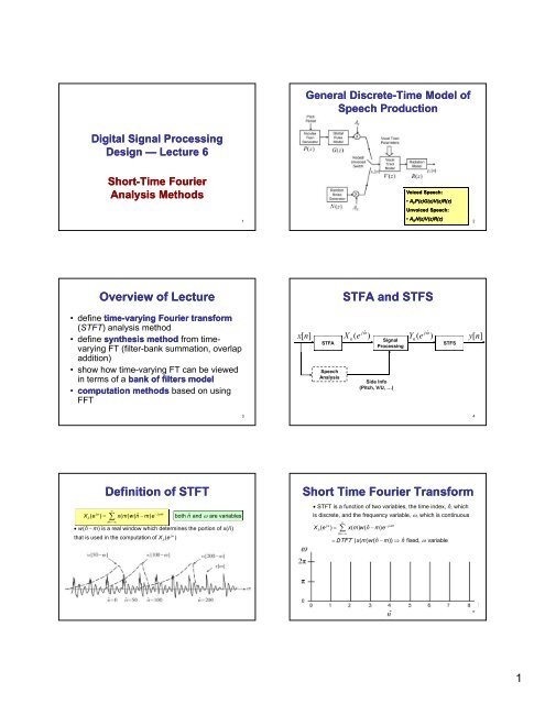
Digital Signal Processing
Design g — Lecture 6
Short Short-Time Time Fourier
Analysis Methods
Overview of Lecture
• define time time-varying varying Fourier transform
(STFT) analysis method
• define synthesis method from timevarying
y g FT ( (filter-bank summation, , overlap p
addition)
• show how time-varying FT can be viewed
in terms of a bank of filters model
• computation methods based on using
FFT
Definition of STFT
∞
∑
jω − jωm X ˆ ˆ
nˆ
( e ) = x( m) w( n−m) e both n and ω are variables
m=−∞
• wn ( ˆ −m)
is a real window which determines the portion of xn ( ˆ)
jω
that is used in the computation of X ( e )
nˆ
1
3
5
x[ n]
General Discrete Discrete-Time Time Model of
Speech Production
STFA
Speech
Analysis
Voiced Speech:
• AVP(z)G(z)V(z)R(z) P(z)G(z)V(z)R(z)
Unvoiced Speech:
• ANN(z)V(z)R(z) N(z)V(z)R(z)
STFA and STFS
X e
j ˆ ω
n(
)
Signal
Processing
n
j ˆ
Side Info
(Pitch, V/U, …)
Y ( e )
ω
STFS
Short Time Fourier Transform
• STFT is a function of two variables, the time index, nˆ
, which
is discrete, and the frequency variable, ω,
which is continuous
nˆ
∞
jω = ∑
m=−∞
ˆ −
− jωm X ( e ) x( m) w( n m) e
= DTFT ( xmwn ( ) ( ˆ −m)) ⇒ nˆ
fixed, ω variable
nˆ
2
yn [ ]
4
6
1

Interpretations of STFT
jω
• there are 2 distinct interpretations of X ( e )
jω
1.
assume nˆis fixed, then Xnˆ( e ) is simply the normal Fourier
transform of the sequence wn ( ˆ −mxm ) ( ), −∞ < m<
∞ => for
jω
fixed nˆ, X ˆ ( e ) has the same
properties as a normal Fourier
n
transform a s o
j ˆ ω
2. consider Xn( e ) as a function of the time index n with ˆ ω fixed.
j ˆ ω − j ˆ ωn
Then Xn( e ) is in the form of a convolution of the signal x( n) e
with the window
wn ( ). This leads to an interpretation in the form of
− j ˆ ωn
linear filtering of the frequency modulated signal xne ( ) by wn ( ).
- we will now consider each of these interpretations of the STFT in
a lot more detail
Signal Recovery from STFT
jω
• since for a given value of nX ˆ,
nˆ
( e ) has the same properties as a
normal Fourier transform, we can recover the input sequence exactly
jω
• since Xnˆ( e ) is the normal Fourier transform of the windowed
sequence wn ( ˆ − mxm ) ( ), then
π
1
j jω j jωm wn ( ˆ − mxm ) ( ) =
2 ∫ ˆ ( ) ω
π ∫ Xn e e d
−π
• assuming the window satisfies the property that w(
0) ≠ 0 ( a trivial
requirement), then by evaluating the inverse Fourier transform
when m = nˆ,
we obtain
π
1
jω jωnˆ xn ( ˆ)
= ˆ(
) ω
2 ( 0)
∫ Xn e e d
w
π −π
Alternative Forms of STFT
jω
Alternative forms of X ( e )
n
1.
real and imaginary parts
jω jω jω
X = ⎡
⎣
⎤
⎦
+ ⎡
⎣
⎤
n( e ) Re Xn( e ) jIm Xn( e )
⎦
= an( ω) − jbn(
ω)
jω
a ( ω)
= Re ⎣
⎡ ( ) ⎦
⎤
n n( ) ⎣X n n(
e ) ⎦
jω
b ( ω)
=−Im ⎡
⎣ ( ) ⎤
n Xn e ⎦
• when xm ( ) and wn ( −m)
are both real (usually the case)
can show that an( ω) is symmetric in ω, and bn(
ω)
is
anti-symmetric in ω
2. magnitude and phase
jω jω
jθn(
ω)
Xn( e ) = | Xn( e ) | e
jω
• can relate | X ( e ) | and θ ( ω) to a ( ω) and b ( ω)
nˆ
n n n n
7
9
11
Frequencies for STFT
• the STFT is periodic in ω with period 2 π,
i.e.,
jω j( ω+ 2πk)
Xnˆ( e ) = Xnˆ( e ), ∀k
• can use any of several frequency variables to express STFT,
including
ω =ΩT (where T is the sampling period for x( m))
to represent
jΩT analog radian frequency, giving Xn( e )
ω = 2πf or ω = 2πFT to represent normalized frequency (0 ≤f ≤1)
j2πf j2πFT or analog frequency (0 ≤F ≤ F = / T), giving X ( e ) or X ( e )
s 1 nˆ nˆ
Signal Recovery from STFT
π
1
jω jωnˆ xn ( ˆ)
=
ˆ ( ) ω
2π( 0)
∫ Xn e e d
w −π
• with the requirement that w( 0) ≠ 0,
the sequence x( nˆ)
jω jω
can be recovered exactly from Xnˆ( e ), if Xnˆ( e ) is known
for all values of ω over one complete period
- sample-by-sample recovery process
jω
- X ˆ
nˆ
( e ) must be known for every value of n and for all ω
i can also recover sequence wn ( ˆ − mxm ) ( ) but can't guarantee
that xm ( ) can be recovered since wn ( ˆ − m) can
equal 0
Windows in STFT
jω
• for Xn( e ) to represent the short-time spectral properties of x( n)
jθ
inside the window => We ( ) should be much narrower in frequency
jω
than significant spectral regions of Xe ( )--i.e., almost an impulse
in frequency
• consider rectangular g and Hamming g windows, where width of the
main spectral lobe is inversely proportional to window length, and side
lobe levels are essentially independent of window length
Rectangular Window: flat window of length L samples; first
zero in frequency response occurs at FS/L, with sidelobe levels
of -14 dB or lower
Hamming Window: raised cosine window of length L
samples; first zero in frequency response occurs at 2FS/L, with
sidelobe levels of -40 dB or lower
8
10
12
2

Time and Frequency Responses of
L=2M+1 Point Hamming Window
Effect of Window Length Length-HW HW
Effect of Window Length Length-HW HW
13
15
17
Effect of Window Length
Effect of Window Length Length-RW RW
Linear Filtering Interpretation
1.
modulation-lowpass filter form
n(
∞
j ˆ ω
) = ∑
m=−∞
( )
− j ˆ ωm
( − )
X e x m e w n m
− j ˆ ωn
( )
π
∫
= wn ( ) ∗ xne ( ) , nvariable,
ˆ ω fixed
1
j jθθ j ( θθ + ˆ ωω ) j jθθ n
= We ( ) Xe ( ) e d dθθ
2π
−π
2.
bandpass filter-demodulation
n(
∞
j ˆ ω
) = ∑
m=−∞
( ) ( − )
−j ˆ ω(
n−m) =
∞
− j ˆ ωn ∑
m=−∞
j ˆ ωm
−
− j ˆ ωn j ˆ ωn
X e w m x n m e
e ( w( m) e ) x( n m)
= e [( w( n) e ) ∗x(
n)], n
variable, ˆ ω fixed
14
16
18
3

Linear Filtering Interpretation
1. modulation-lowpass filter form:
∞
j ˆ ω
n(
) = ∑
m=−∞
(
− j ˆ ωm
) ( − ), variable, ˆ ω fixed
X e x m e w n m n
− jωn ( xne ( ) ) wn ( )
( ˆ ω ) ( ˆ ω )
= ∗
= xn ( )cos( n) ∗wn ( ) − j xn ( )sin( n) ∗wn
( )
= a ( ˆ ω) − jb ( ˆ ω)
n n
Linear Filtering Interpretation
Sampling Rate in Time
• to determine the sampling rate in time, we take a linear filtering view
j ˆ ω
1. Xn( e ) is the output of a filter with impulse response w( n)
jω
2. We ( ) is a lowpass response with effective bandwidth
of B Hertz
j ˆ ω j ˆ ω
• thus the effective bandwidth of Xn( e ) is B Hertz => Xn( e ) has
to be sampled at a rate of 2B
samples/second to avoid aliasing
Example: Hamming Window ( L = 100 samples; L = 400 samples)
2Fs
⇒B ≈ (Hz); for L = 100, Fs= 10, 000 Hz => B = 200 Hz => need
L
rate of 400/sec (every R = 25 samples) for sampling rate in time (wideband analysis)
⇒ for L = 400, FS= 10, 000 Hz ⇒ B = 50 Hz ⇒ need rate of R = 100/sec
(every 100 samples) for sampling rate in time (narrowband analysis)
19
21
23
Linear Filtering Interpretation
2. bandpass filter-demodulation form
X e
−
e ⎡
⎣( w n e ) x n ⎤
⎦
n
j ˆ ω j ˆ ωn j ˆ ωn
n(
) = ( ) ∗ ( ) , variable, ω fixed
• complex bandpass filter output
− jωn modulated by signal e
jθ
• if We ( ) is lowpass, then filter
is bandpass around θ = ω
• all real computation for lower
half structure
Sampling Rates of STFT
• need to sample STFT in both time and frequency to
produce an unaliased representation from which x(n) can
be exactly recovered
• sampling rates lower than the theoretical minimum rate
can be used, in either time or frequency, and x(n) can
still till bbe exactly tl recovered dffrom th the aliased li d( (under- d
sampled) short-time transform
– this is useful for spectral estimation, pitch estimation, formant
estimation, speech spectrograms, vocoders
– for applications where the signal is modified, e.g., speech
enhancement, cannot undersample STFT and still recover
modified signal exactly
Sampling Rate in Frequency
jω
• since Xnˆ( e ) is periodic in ω with period 2π,
it is only necessary to sample over an
interval of length 2π
• need to determine an appropriate finite set of frequencies, ωk= 2π k / N, k = 01 , ,..., N −1
jω
at which Xnˆ( e ) must be specified to exactly recover x( n)
jω
• use the Fourier transform interpretation of Xnˆ( e )
jω
1. if the window wn ( ) is time-limited, then the inverse transform of Xnˆ( e ) is time-limited
j jωω
22. the sampling theorem requres that we sample X Xnˆ ( e ) in the frequency dimension ata at a
rate of at least twice its ('symmetric') "time width"
jω
3. since the inverse Fourier transform of X ˆ
ˆ ( e ) is the signal x( m) w( n−m) and this signal
n
is of duration L samples (the duration of w( n)),
then according to the sampling theorem
jω
Xnˆ( e ) must be sampled (in frequency) at the set of frequencies
2π
k
ω k = , k = 01 , ,..., L−1(where L/
2 is the effective width of the window)
L
jωk
in order to exactly recover xn ( ) from X ˆ ( e ) (see Prob. 6.8)
n
• thus for a Hamming window of duration L=100 samples, we require that the STFT be
evaluated at at least 100 uniformly spaced frequencies around the unit circle
ˆ
20
22
24
4

“Total” Sampling Rate of STFT
• the “total” sampling rate for the STFT is the product of the sampling
rates in time and frequency, i.e.,
SR = SR(time) x SR(frequency)
= 2B x L samples/sec
B = frequency bandwidth of window (Hz)
L = time width of window (samples)
• for most windows of interest, , B is a multiple p of FS/L, S , i.e., ,
B = C FS/L (Hz), C=1 for Rectangular Window
C=2 for Hamming Window
SR = 2C FS samples/second
• can define an ‘oversampling rate’ of
SR/ FS = 2C = oversampling rate of STFT as compared to
conventional sampling representation of x(n)
for RW, 2C=2; for HW 2C=4 => range of oversampling is 2-4
this oversampling gives a very flexible representation of the speech signal
Spectrographic Displays
• Sound Spectrograph-one of the earliest embodiments of the timedependent
spectrum analysis techniques
– 2-second utterance repeatedly modulates a variable frequency
oscillator, then bandpass filtered, and the average energy at a given
time and frequency is measured and used as a crude measure of the
STFT
– thus energy is recorded by an ingenious electro-mechanical system on
special electrostatic paper called teledeltos paper
– result is a two-dimensional representation of the time-dependent
spectrum-with vertical intensity being spectrum level at a given
frequency, and horizontal intensity being spectral level at a given timewith
spectrum magnitude being represented by the darkness of the
marking
– wide bandpass filters (300 Hz bandwidth) provide good temporal
resolution and poor frequency resolution (resolve pitch pulses in time
but not in frequency)—called wideband spectrogram
– narrow bandpass filters (45 Hz bandwidth) provide good frequency
resolution and poor time resolution (resolve pitch pulses in frequency,
but not in time)—called narrowband spectrogram
27
Sequence of Spectrograms of Utterance “This is a test”
3 msec (48 sample)
analysis window
25
6 msec (96 sample)
analysis window
9 msec (144 sample)
analysis window
30 msec (480
sample) analysis
window
29
Sampling the STFT
Speech Spectrograms
• wideband spectrogram
• follows broad spectral peaks (formants)
over time
• resolves most individual pitch periods as
vertical striations since the IR of the
analyzing filter is comparable in duration
to a pitch period
• what happens for low pitch males—high
pitch females
• for unvoiced speech there are no vertical
pitch striations
• narrowband spectrogram
• individual harmonics are resolved in
voiced regions
• formant frequencies are still in evidence
• usually can see fundamental frequency
• unvoiced regions show no strong
structure
28
Spectrogram Comparisons
26
30
5

Wideband Spectrogram - Male
nfft = 1024, L = 80 / 800, Overlap = 75 / 790
Overlap Addition (OLA) Method
• based on normal FT interpretation of short-time spectrum
jωk
DFT / IDFT
X ˆ
nˆ( e ) ←⎯⎯⎯⎯→ ynˆ( m) = x( m) w( n−m) jωk
• can reconstruct x(m) by computing IDFT of Xnˆ ( e ) and
dividing out the window (assumed non-zero non zero for all samples)
• this process gives L signal values of x(m) for each window =>
window can be moved by L samples and the process repeated
jωk
• since Xnˆ( e ) is "undersampled" in time, it is highly susceptible
to aliasing errors => need more robust synthesis procedure
Overlap Addition of Bartlett and Hann
Windows
31
33
35
Wideband Spectrogram - Female
nfft = 1024, L = 80 / 800, Overlap = 75 / 790
Overlap Addition (OLA) Method
⎡ jω ω ⎤
k j kn
yn ( ) = ∑∑ ⎢ Xm( e ) e ⎥
m ⎣ k
⎦
• summation is for overlapping analysis sections
jωk
• for each value of m where Xm( e ) is measured, do an inverse FT to give
ym( n) = Lx( n) w( m−n) (where L is the size of the FT)
y ( n ) = y ( n ) = Lx ( n ) w ( m m− n )
∑ m ∑
m m
• a basic property of the window is
N−1
j 0
jωk
We ( ) = We ( )| ω = 0 = ∑wn
( )
k
n=
0
• since any set of samples of the window are equivalent (by sampling arguments),
then if wn ( ) is sampled often
enough we get (independent of n)
j 0
∑wm
( − n) = We ( )
m
j 0
yn ( ) = LxnWe ( ) ( ) using overlap-added sections
Overlap Addition of Hamming Window
L=128
32
34
36
6

Overlap Addition (OLA) Method
Filter Bank Summation
• the filter bank interpretation of the STFT shows that for
jωk
any frequency ωk,
Xn( e ) is a lowpass representation
of the signal in a band centered at ω
n( ∞
jωk − jωkn ) = ∑
m=−∞
( − )
k
k(
)
jωkm X e e x n m w m e
where wk( m)
is the lowpass window used at frequency ωk
(we have generalized the structure to allow a different
lowpass window at each frequency ω ).
Filter Bank Summation
jωk
• thus Xn( e ) is obtained by bandpass filtering x( n)
followed by modulation with the complex exponential
− jωkn e . We can express this in the form
jωk jωkn y ( n) = X ( e ) e = x( n−m) h ( m)
k n k
m=−∞
• thus yk( n)
is the output of a bandpass filter with impulse
response h ( n)
k
∞
∑
k
37
39
41
Overlap Addition (OLA) Method
• 4-overlapping sections
contribute to each interval
• N-point FFT’s done using
L speech p samples, p , with N-L
zeros padded at end to
allow modifications without
significant aliasing effects
• for a given value of n
y(n)=x(n)w(R-n)+x(n)w(2Rn)+x(n)w(3R-n)+x(n)w(4Rn)=x(n)[w(R-n)+w(2Rn)+w(3R-n)+w(4R-n)]=x(n)
W(ej0 )/R
Filter Bank Summation
• define a bandpass filter and substitute it in the
equation to give
ωk
h ( n) = w ( n) e
k k
j n
jωk − jωkn X ( e ) = e x( n−m) h ( m)
n k
m=−∞
∞
∑
Filter Bank Summation
38
40
42
7

Filter Bank Summation
Filter Bank Summation
• consider a set of N bandpass filters, uniformly spaced, so that the entire
frequency band is covered
2π
k
ωk
= , k = 01 , ,..., N −1
N
• also assume window the same for all channels, i.e.,
w wk ( n ) = w ( n n)
), k = 01 , ,..., N − 1
• if we add together all the bandpass outputs, the composite response is
N−1 N−1
jω jω
j(
ω−ωk) He ( ) = ∑Hk( e ) = ∑We
( )
k= 0 k=
0
jωk
• if We ( ) is properly sampled in frequency ( N≥ L), where Lis
the
window duration, then it can be shown that
N−1
1
j(
ω−ωk) ∑We
( ) = w(
0)
∀ω
N
FBS Formula
k = 0
45
Filter Bank Summation
• derivation of FBS formula
FT / IFT jω
wn ( ) ←⎯⎯⎯→We
( )
jω
• if We ( ) is sampled in frequency at Nuniformly
spaced p p points, , the inverse discrete Fourier transform
jωk
of the sampled version of We ( ) is (recall that
sampling ⇒ multiplication ⇔ convolution ⇒ aliasing)
N−1
∑
jωk jωkn ∞
∑
k= 0
r=−∞
1
N
We ( ) e = wn ( + rN)
• an aliased version of wn ( ) is obtained.
43
47
Filter Bank Summation
• a practical method for reconstructing xn ( ) from the STFT is as follows
jωk
1. assume we know Xn( e ) for a set of N frequencies { ωk},
k = 01 , ,..., N −1
2. assume we have a set of N bandpass filters with impulse responses
jωkn hk( n) = wk( n) e , k = 01 , ,..., N −1
3. assume wk( n)
is an ideal lowpass filter with cutoff frequency ωpk
- the frequency response of the bandpass filter is
jω
j(
ω−ωk) Hk( e ) = Wk( e )
Filter Bank Summation
Filter Bank Summation
• If wn ( ) is of duration Lsamples,
then
wn ( ) = 0, n< 0,
n≥ L
• and no aliasing occurs due to sampling in frequency
jω
of We ( ). In this case if we evaluate the aliased
formula for n = 0 0,
we get
N−1
1
jωk
∑We
( ) = w(
0)
N
k = 0
• the FBS formula is seen to be equivalent to the formula
above, since (according to the sampling theorem) any
jω
set of N uniformly spaced samples of W( e
) is adequate
44
46
48
8

Filter Bank Summation
• the impulse response of the composite filter bank system is
N−1 N−1
jωkn hn ( ) = ∑hk( n) = ∑wne
( ) = Nw( 0)
δ ( n)
k= 0 k=
0
• thus the composite output is
yn ( ) = xn ( ) ∗ h h ( n ) = N w ( 0 ) x ( n )
• thus for FBS method, the reconstructed signal is
N−1 N−1
jωk jωkn yn ( ) = ∑yk( n) = ∑Xn( e ) e = Nw( 0)
xn ( )
k= 0 k=
0
jωk
• if Xn( e ) is sampled properly in frequency, and is independent of the
shape of wn ( )
Filter Bank Summation
N−1 = ∑ k
N−1
= ∑ n
2π j k
N
2π
j kn
N
k= 0 k=
0
N−1
2π 2π
⎡ − j km⎤ j kn
N N
= ∑∑ ⎢ xmwn ( ) ( −me
) ⎥ e
k= 0 ⎣ m
⎦
N −1
2π
j k( n−m) N
= ∑ ∑xmwn ( ) ( −m)
∑ ∑e
m k=
0
∞
yn ( ) y( n) X( e ) e
∑ ∑
∑
= xmwn ( ) ( −m) Nδ( n−m−rN) m r=−∞
∞
y( n) = N w( rN) x( n −rN)
r =−∞
•wn ( ) ≠ 0 for 0≤n≤L−1⇒ if N≥Lthen need
only r = 0 term
y(n) = Nw( 0)x(n)
• if N < L then in order for y( n) = x( n) you need the condition w( rN) = 0, r = ± 1, ± 2,...
• 'undersampled' representation can still work--at least in theory
FBS Reconstruction in Non- Non
Overlapping Bands
• assume window length for all bands is L samples
• assume the same window is used for N equally spaced
frequency bands with analysis frequencies
2π
k
ωk
= , k = 01 , ,..., N −1
N
• where N can be less than L
• assume w(n) is an ideal lowpass filter with cutoff frequency
π
ωp
=
N
example with N=6
equally spaced ideal
filters
49
51
53
Filter Bank Summation
Summary of FBS Method
jω
• perfect reconstruction of x(n) from Xn ( e ) is possible using FBS
under the following conditions:
1. w(n) is a finite duration filter/window
jω
2. Xn( e ) is sampled properly in both time
and frequency
j k
perfect reconstruction of x(n) from Xn ( e ) is also possible using
FBS under the following condition:
ω
•
FBS under the following condition:
jω
We ( ) is perfectly bandlimited
jωk
• To avoid time aliasing, Xn( e ) must be evaluated at at least L uniformly spaced
frequencies, where L is the window duration
-since window of length L samples has frequency bandwidth of from
2π / L (for RW) to 4π
/ L (for HW), the bandpass filters in FBS overlap
in frequency since the analysis frequencies are 2 k/ L, k 01 , ,..., L 1
j k
there is a way (at least theoretically) for Xn( e ) to be evaluated in
non-overlapping bands
52
ω
π = −
•
and for which x(n) can still be exactly recovered
FBS Reconstruction in Non- Non
Overlapping Bands
• the composite impulse response for the FBS system is
N−1 N−1
jωkn jωkn hn ( ) = ∑wne ( ) = wn ( ) ∑ e
k= 0 k=
0
• defining a composite of the terms being summed as
N−1 N−1
jωkn j2πkn/ N
pn ( ) = ∑ e = ∑ e
k= 0 k=
0
• we get for
hn (
)
hn (
) = wn ( ) pn ( )
• it is easy to show (Prob. 6.7) that p(n) is a periodic train of impulses of the form
∞
pn ( ) = N∑ δ(
n−rN) r =−∞
• giving for hn (
) the expression
∞
hn (
) = N∑ wrN ( ) δ ( n−rN) r =−∞
• thus the composite impulse response is the window sequence sampled
at intervals of N
samples
50
54
9

FBS Reconstruction in Non- Non
Overlapping Bands
impulse response of ideal lowpass filter
with cutoff frequency π/N
• for ideal LPF we have
sin( ππ n / N ) sin( ππ
r ) 1
w[n]= [ ] , wrN [ N]
] = = δδ
[ r ]
πN πrN
N
giving hn [
] = δ [ n]
• other cases where perfect reconstruction is obtained
1. wn [ ] is of finite length L< Nand
causal (no images)
2. wn [ ] has length > N and has the property
wn [ ] = 1 / N, for n= rN 0
= 0 for n = rN ( r ≠ r0, r = 0, ± 1, ± 2,...)
giving hn [
] = pnwn [ ] [ ] = δ [ n−rN 0 ]
jω
− jωr0N He ( ) = e ⇒ yn [ ] = xn ( −rN
0 ]
55
Practical Implementation of FBS
Filter Bank Reconstruction
• frequency domain equations
ˆ 1
Ye ( ) PkFe ( ) ( )
N−1
2π
j( ω−
k)
jω N
= ∑
⋅
N k = 0
R 1
2π 2π 2π
⎡ − 1
j( ω− k− ) j(
ω−
)
⎤
N R R
⎢ ∑ ∑We
( ) Xe ( ) ⎥
⎣ R =
0
⎦
N−1
2π 2π
1
j( ω− k) j( ω−
k)
jω N N
= Xe ( ) ∑PkFe
( ) ( ) We ( )
RN k = 0
R−1
2π
j( ω− )
N−1
2π 2π 2π
1
j(
ω−
k) j( ω−
k−
)
R
N N R
+ ∑ Xe ( ) ⋅ ∑PkFe
( ) ( We
=
1
RN k = 0
jω jω
= He (
) ⋅ Xe ( ) + aliasing terms
57
) ( )
59
x(n)
Summary of FBS Reconstruction
• for perfect reconstruction using FBS methods
1. w(n) does not need to be either time-limited
or frequency-limited to exactly reconstruct
jωk
x(n) from Xn ( e )
2. w(n) just needs equally
spaced zeros, spaced
N samples apart for theoretically perfect reconstruction
• exact reconstruction of the input is possible with a
number of frequency channels less than that required
by the sampling theorem
• key issue is how to design digital filters that match these
criteria
Filter Bank Reconstruction
e -j2π0n/N
x
e -j2π1n/N
w(n)
X n(e j2π0/N )
R
X n(e j2π1/N )
Short Timme
Modifications
x w(n) R
R f(n) x
•
•
•
e -j2π(N-1)n/N
•
•
•
•
•
•
X n(e j2π(N-1)/N )
R
f(n)
e j2π0n/N
x w(n) R R f(n) x
X rR(
k)
•
•
•
Xˆ rR ( k)
•
•
•
x
ej2π1n/N P(0)
•
•
•
e j2π(N-1)n/N
P(1)
P(N-1)
yˆ k ( n)
Filter Bank Reconstruction
conditions for perfect reconstruction ( ˆ jω jω
• Ye ( ) = Xe ( ))
and
1
He (
) = PkFe ( ) ( ) We ( ) = 1
1
RN
N−1
2π 2π
j( ω− k) j( ω−
k)
jω N N
∑ RN k=
0
N −1
∑
k = 0
Flat Gain
2π 2π 2π
j( ω− k) j( ω−
k−
)
N N R
PkFe ( ) ( ) We ( ) = 0 for = 12 , ,..., R
Alias Cancellation
+
56
yn ˆ( )
58
60
10

Equivalent Filter Bank
Filter Bank Reconstruction
• consider a linear phase FIR system such that
wn ( ) = wM ( −n), 0 ≤ n≤M = 0 otherwise
• We = W e e
jω jω − jωM / 2
then ( ) real ( ) and
1
2 2
⎡ jω −jωM j( ω−π) −j( ω−π) M
( W ( ) ) − ( ( ) ⎤ ) =
4 ⎢ real e e Wreal e e
⎣ ⎥⎦
1
2 2
⎡ jω −jπM j(
ω−π) ( Wreal ( e ) ) − e ( Wreal ( e ) ⎤ − jωM ) e
4 ⎢⎣ ⎥⎦
− jπM • if M is odd, then e = −1and
we get
1
2 2
⎡ jω j(
ω−π) ( W ( ) ) + ( ( ) ⎤ ) = 1
4 ⎢ real e Wreal e
⎣ ⎥⎦
Quadrature Mirror Filters
Lowpass filter
designed by
windowing
Highpass filter is
mirror image of
lowpass filter
• practical realization of QMF filters
• note that aliasing is cancelled, but the overall frequency
response is not perfectly flat
61
63
65
Filter Bank Reconstruction
• practical solution for the case wn ( ) = fn ( ), N= R=
2 (2-band solution)
where the conditions for exact reconstruction become
1
jω jω j( ω−π) j(
ω−π) ⎡ ( 0) ( ) ( ) + ( 1) ( ) ( ) ⎤ = 1
4 ⎣
P F e W e P F e W e
⎦
and
1
jω j(
ω−π) j( ω−π) j(
ω−2π) ⎡P( 0)
F( e ) W( e 1 0
4 ⎣
) + P( ) F( e ) W( e ) ⎤
⎦
=
jω jω
• aliasing cancels exactly if P( 0) = − P( 1) = 1(with
F( e ) = W( e ))giving
1
2 2
⎡ jω j( ω−π) − ω
( ( ) ) − ( ( ) ⎤ j M
We We ) = e
4 ⎢⎣ ⎥⎦
yn ˆ( ) = xn ( −M)
Quadrature Mirror Filters
jπn h0[ n] = w[ n] = g0[ n] 1 = = 1
h[ n] w[ n] e g [ n]
Tree Tree-Structured Structured QMF Filterbank
62
64
66
11

Discrete Wavelet Transforms
FBS and OLA Comparisons
duals
• filter bank summation method ←⎯⎯⎯→overlap
addition method
-- one depends on sampling relation in frequency
-- one depends on sampling relation in time
• FBS requires sampling in frequency be such that the window
jω
transform We ( ) obeys the relation
N−1
1
j(
ω−ω k )
∑ We ( ) = w ( 0 ) any ωω
N
k = 0
• OLA requires that sampling in time be such that the window
obeys the relation
∞
j 0
∑ wrR ( − n) = We ( )/ R any n
r =−∞
• the key to Short-Time Fourier Analysis is the ability to modify
the short-time spectrum (via quantization, noise enhancement,
signal enhancement, speed-up/slow-down,etc) and recover
an "unaliased" modified signal
67
69
frequency
STFT and CWT
ω0 3ω 5ω 0 0
ω0 2ω0
4ω0
8ω0
time
Constant bandwidth
frequency
Summary
time
Constant-Q bandwidth
• Definition of short-term Fourier transform (STFT):
∞
jω−jωn •
Xn( e ) = ∑ x[ m] w[ n−m] e
m=−∞
– keep ˆn fixed => STFT looks like a standard DFT =>
overlap-add (OLA) synthesis
– keep ωˆω
fixed => STFT looks like a filter bank => filter
bank summation (FBS) synthesis
– sampling rate in time based on window bandwidth;
sampling rate in frequency based on window time width
(length)
– range of synthesis procedures for both FBS and OLA
– STFT sequence can be displayed as an image =>
wideband/narrowband spectrograms
70
68
12