Ch.17: Radiation from Apertures
Ch.17: Radiation from Apertures
Ch.17: Radiation from Apertures

Create successful ePaper yourself
Turn your PDF publications into a flip-book with our unique Google optimized e-Paper software.
17.1 Field Equivalence Principle<br />
17<br />
<strong>Radiation</strong> <strong>from</strong> <strong>Apertures</strong><br />
The radiation fields <strong>from</strong> aperture antennas, such as slots, open-ended waveguides,<br />
horns, reflector and lens antennas, are determined <strong>from</strong> the knowledge of the fields<br />
over the aperture of the antenna.<br />
The aperture fields become the sources of the radiated fields at large distances. This<br />
is a variation of the Huygens-Fresnel principle, which states that the points on each<br />
wavefront become the sources of secondary spherical waves propagating outwards and<br />
whose superposition generates the next wavefront.<br />
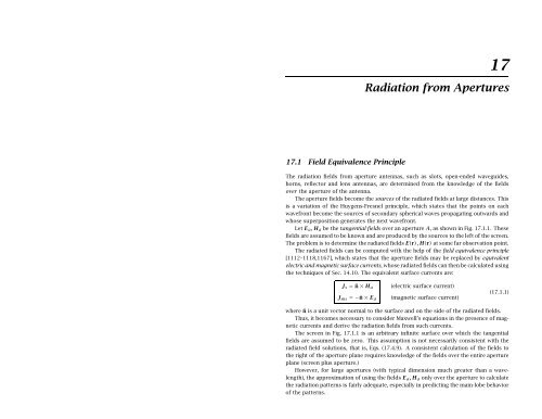
Let E a, H a be the tangential fields over an aperture A, as shown in Fig. 17.1.1. These<br />
fields are assumed to be known and are produced by the sources to the left of the screen.<br />
The problem is to determine the radiated fields E(r), H(r) at some far observation point.<br />
The radiated fields can be computed with the help of the field equivalence principle<br />
[1112–1118,1167], which states that the aperture fields may be replaced by equivalent<br />
electric and magnetic surface currents, whose radiated fields can then be calculated using<br />
the techniques of Sec. 14.10. The equivalent surface currents are:<br />
J s = ˆn × H a<br />
J ms =−ˆn × E a<br />
(electric surface current)<br />
(magnetic surface current)<br />
(17.1.1)<br />
where ˆn is a unit vector normal to the surface and on the side of the radiated fields.<br />
Thus, it becomes necessary to consider Maxwell’s equations in the presence of magnetic<br />
currents and derive the radiation fields <strong>from</strong> such currents.<br />
The screen in Fig. 17.1.1 is an arbitrary infinite surface over which the tangential<br />
fields are assumed to be zero. This assumption is not necessarily consistent with the<br />
radiated field solutions, that is, Eqs. (17.4.9). A consistent calculation of the fields to<br />
the right of the aperture plane requires knowledge of the fields over the entire aperture<br />
plane (screen plus aperture.)<br />
However, for large apertures (with typical dimension much greater than a wavelength),<br />
the approximation of using the fields E a, H a only over the aperture to calculate<br />
the radiation patterns is fairly adequate, especially in predicting the main-lobe behavior<br />
of the patterns.
17.1. Field Equivalence Principle 659<br />
Fig. 17.1.1 Radiated fields <strong>from</strong> an aperture.<br />
The screen can also be a perfectly conducting surface, such as a ground plane, on<br />
which the aperture opening has been cut. In reflector antennas, the aperture itself is<br />
not an opening, but rather a reflecting surface. Fig. 17.1.2 depicts some examples of<br />
screens and apertures: (a) an open-ended waveguide over an infinite ground plane, (b)<br />
an open-ended waveguide radiating into free space, and (c) a reflector antenna.<br />
Fig. 17.1.2 Examples of aperture planes.<br />
There are two alternative forms of the field equivalence principle, which may be used<br />
when only one of the aperture fields E a or H a is available. They are:<br />
J s = 0<br />
J ms =−2(ˆn × E a)<br />
J s = 2(ˆn × H a)<br />
J ms = 0<br />
(perfect magnetic conductor) (17.1.2)<br />
(perfect electric conductor) (17.1.3)<br />
They are appropriate when the screen is a perfect electric conductor (PEC) on which<br />
E a = 0, or when it is a perfect magnetic conductor (PMC) on which H a = 0.<br />
660 17. <strong>Radiation</strong> <strong>from</strong> <strong>Apertures</strong><br />
Using image theory, the perfect electric (magnetic) conducting screen can be eliminated<br />
and replaced by an image magnetic (electric) surface current, doubling its value<br />
over the aperture. The image field causes the total tangential electric (magnetic) field to<br />
vanish over the screen.<br />
If the tangential fields E a, H a were known over the entire aperture plane (screen plus<br />
aperture), the three versions of the equivalence principle would generate the same radiated<br />
fields. But because we consider E a, H a only over the aperture, the three versions<br />
give slightly different results.<br />
In the case of a perfectly conducting screen, the calculated radiation fields (17.4.10)<br />
using the equivalent currents (17.1.2) are consistent with the boundary conditions on<br />
the screen.<br />
17.2 Magnetic Currents and Duality<br />
Next, we consider the solution of Maxwell’s equations driven by the ordinary electric<br />
charge and current densities ρ, J, and in addition, by the magnetic charge and current<br />
densities ρm, J m.<br />
Although ρm, J m are fictitious, the solution of this problem will allow us to identify<br />
the equivalent magnetic currents to be used in aperture problems, and thus, establish<br />
the field equivalence principle. The generalized form of Maxwell’s equations is:<br />
∇×H = J + jωɛE<br />
∇·E = 1<br />
ɛ ρ<br />
∇×E =−J m − jωμH<br />
∇·H = 1<br />
μ ρm<br />
(17.2.1)<br />
There is now complete symmetry, or duality, between the electric and the magnetic<br />
quantities. In fact, it can be verified easily that the following duality transformation<br />
leaves the set of four equations invariant:<br />
E −→ H<br />
H −→ −E<br />
ɛ −→ μ<br />
μ −→ ɛ<br />
J −→ J m<br />
ρ −→ ρm<br />
J m −→ −J<br />
ρm −→ −ρ<br />
A −→ A m<br />
ϕ −→ ϕm<br />
A m −→ −A<br />
ϕm −→ −ϕ<br />
(duality) (17.2.2)<br />
where ϕ, A and ϕm, A m are the corresponding scalar and vector potentials introduced<br />
below. These transformations can be recognized as a special case (for α = π/2) of the<br />
following duality rotations, which also leave Maxwell’s equations invariant:<br />
<br />
′ ′ ′<br />
E ηJ ηρ<br />
ηH ′<br />
J ′ m ρ ′ <br />
cos α sin α E ηJ ηρ<br />
=<br />
(17.2.3)<br />
m − sin α cos α ηH Jm ρm<br />
Under the duality transformations (17.2.2), the first two of Eqs. (17.2.1) transform<br />
into the last two, and conversely, the last two transform into the first two.
17.2. Magnetic Currents and Duality 661<br />
A useful consequence of duality is that if one has obtained expressions for the electric<br />
field E, then by applying a duality transformation one can generate expressions for<br />
the magnetic field H. We will see examples of this property shortly.<br />
The solution of Eq. (17.2.1) is obtained in terms of the usual scalar and vector potentials<br />
ϕ, A, as well as two new potentials ϕm, A m of the magnetic type:<br />
E =−∇ϕ − jωA − 1<br />
ɛ ∇×A m<br />
H =−∇ϕm − jωA m + 1<br />
μ ∇×A<br />
(17.2.4)<br />
The expression for H can be derived <strong>from</strong> that of E by a duality transformation of<br />
the form (17.2.2). The scalar and vector potentials satisfy the Lorenz conditions and<br />
Helmholtz wave equations:<br />
∇·A + jωɛμ ϕ = 0<br />
∇ 2 ϕ + k 2 ϕ =− ρ<br />
ɛ<br />
∇ 2 A + k 2 A =−μJ and<br />
∇·A m + jωɛμ ϕm = 0<br />
∇ 2 ϕm + k 2 ϕm =− ρm<br />
μ<br />
∇ 2 A m + k 2 A m =−ɛ J m<br />
(17.2.5)<br />
The solutions of the Helmholtz equations are given in terms of G(r − r ′ )= e−jk|r−r′ |<br />
4π|r − r ′ | :<br />
<br />
ϕ(r) =<br />
V<br />
1<br />
ɛ ρ(r′ )G(r − r ′ )dV ′ ,<br />
<br />
A(r) = μ J(r<br />
V<br />
′ )G(r − r ′ )dV ′ ,<br />
<br />
ϕm(r) =<br />
V<br />
1<br />
μ ρm(r ′ )G(r − r ′ )dV ′<br />
<br />
A m(r) = ɛ J m(r<br />
V<br />
′ )G(r − r ′ )dV ′<br />
(17.2.6)<br />
where V is the volume over which the charge and current densities are nonzero. The<br />
observation point r is taken to be outside this volume. Using the Lorenz conditions, the<br />
scalar potentials may be eliminated in favor of the vector potentials, resulting in the<br />
alternative expressions for Eq. (17.2.4):<br />
E = 1 <br />
∇(∇·A)+k<br />
jωμɛ<br />
2 A − 1<br />
ɛ ∇×A m<br />
H = 1 <br />
∇(∇·A m)+k<br />
jωμɛ<br />
2 1<br />
A m +<br />
μ ∇×A<br />
These may also be written in the form of Eq. (14.3.9):<br />
E = 1 <br />
∇×(∇×A)−μ J]−<br />
jωμɛ<br />
1<br />
ɛ ∇×A m<br />
H = 1 <br />
∇×(∇×A m)−ɛ J m]+<br />
jωμɛ<br />
1<br />
μ ∇×A<br />
(17.2.7)<br />
(17.2.8)<br />
662 17. <strong>Radiation</strong> <strong>from</strong> <strong>Apertures</strong><br />
Replacing A, A m in terms of Eq. (17.2.6), we may express the solutions (17.2.7) directly<br />
in terms of the current densities:<br />
E = 1<br />
<br />
<br />
2<br />
k J G + (J ·∇<br />
jωɛ<br />
′ )∇ ′ G − jωɛ J m ×∇ ′ G dV ′<br />
H = 1<br />
jωμ<br />
<br />
V<br />
V<br />
k 2 J m G + (J m ·∇ ′ )∇ ′ G + jωμ J ×∇ ′ G dV ′<br />
Alternatively, if we also use the charge densities, we obtain <strong>from</strong> (17.2.4):<br />
<br />
E =<br />
−jωμ J G + ρ<br />
ɛ ∇′ G − J m ×∇ ′ G dV ′<br />
V<br />
<br />
<br />
H = −jωɛ J m G +<br />
V<br />
ρm<br />
μ ∇′ G + J ×∇ ′ G dV ′<br />
17.3 <strong>Radiation</strong> Fields <strong>from</strong> Magnetic Currents<br />
(17.2.9)<br />
(17.2.10)<br />
The radiation fields of the solutions (17.2.7) can be obtained by making the far-field<br />
approximation, which consists of the replacements:<br />
e −jk|r−r′ |<br />
4π|r − r ′ |<br />
≃ e−jkr<br />
4πr ejk·r′<br />
and ∇≃−jk (17.3.1)<br />
where k = kˆr. Then, the vector potentials of Eq. (17.2.6) take the simplified form:<br />
A(r)= μ e−jkr<br />
4πr F(θ, φ) , A m(r)= ɛ e−jkr<br />
4πr Fm(θ, φ) (17.3.2)<br />
where the radiation vectors are the Fourier transforms of the current densities:<br />
<br />
F(θ, φ) =<br />
<br />
Fm(θ, φ) =<br />
J(r<br />
V<br />
′ )e jk·r′<br />
dV ′<br />
J m(r<br />
V<br />
′ )e jk·r′<br />
dV ′<br />
(radiation vectors) (17.3.3)<br />
Setting J = J m = 0 in Eq. (17.2.8) because we are evaluating the fields far <strong>from</strong> the<br />
current sources, and using the approximation ∇=−jk =−jkˆr, and the relationship<br />
k/ɛ = ωη, we find the radiated E and H fields:<br />
E =−jω e<br />
ˆr × (A × ˆr)−ηˆr × A m =−jk −jkr<br />
4πr ˆr × <br />
ηF × ˆr − Fm<br />
H =− jω<br />
ηˆr × (A m × ˆr)+ˆr × A<br />
η<br />
=− jk e<br />
η<br />
−jkr<br />
4πr ˆr × ηF + Fm × ˆr <br />
These generalize Eq. (14.10.2) to magnetic currents. As in Eq. (14.10.3), we have:<br />
(17.3.4)<br />
H = 1<br />
ˆr × E (17.3.5)<br />
η
17.4. <strong>Radiation</strong> Fields <strong>from</strong> <strong>Apertures</strong> 663<br />
Noting that ˆr × (F × ˆr)= ˆ θFθ + ˆ φFφ and ˆr × F = ˆ φFθ − ˆ θFφ, and similarly for Fm,<br />
we find for the polar components of Eq. (17.3.4):<br />
E =−jk e−jkr <br />
ˆθ(ηFθ + Fmφ)+<br />
4πr<br />
ˆ φ(ηFφ − Fmθ) <br />
H =− jk<br />
η<br />
e−jkr <br />
−θ(ηFφ ˆ − Fmθ)+<br />
4πr<br />
ˆ φ(ηFθ + Fmφ) <br />
The Poynting vector is given by the generalization of Eq. (15.1.1):<br />
P= 1<br />
2 Re(E × H∗ )= ˆr<br />
and the radiation intensity:<br />
k2 32π2ηr2 |ηFθ + Fmφ| 2 +|ηFφ − Fmθ| 2 = ˆr Pr<br />
U(θ, φ)= dP<br />
dΩ = r2Pr = k2<br />
32π2 <br />
|ηFθ + Fmφ|<br />
η<br />
2 +|ηFφ − Fmθ| 2<br />
17.4 <strong>Radiation</strong> Fields <strong>from</strong> <strong>Apertures</strong><br />
(17.3.6)<br />
(17.3.7)<br />
(17.3.8)<br />
For an aperture antenna with effective surface currents given by Eq. (17.1.1), the volume<br />
integrations in Eq. (17.2.9) reduce to surface integrations over the aperture A:<br />
E = 1<br />
<br />
<br />
(J s ·∇<br />
jωɛ A<br />
′ )∇ ′ G + k 2 J s G − jωɛ J ms ×∇ ′ G dS ′<br />
H = 1<br />
jωμ<br />
<br />
A<br />
(J ms ·∇ ′ )∇ ′ G + k 2 J ms G + jωμ J s ×∇ ′ G dS ′<br />
and, explicitly in terms of the aperture fields shown in Fig. 17.1.1:<br />
E = 1<br />
<br />
jωɛ<br />
H = 1<br />
jωμ<br />
<br />
A<br />
A<br />
(ˆn × H a)·∇ ′ (∇ ′ G)+k 2 (ˆn × H a)G + jωɛ(ˆn × E a)×∇ ′ G dS ′<br />
−(ˆn × E a)·∇ ′ (∇ ′ G)−k 2 (ˆn × E a)G + jωμ(ˆn × H a)×∇ ′ G dS ′<br />
(17.4.1)<br />
(17.4.2)<br />
These are known as Kottler’s formulas [1116–1121,1111,1122–1126]. We derive them<br />
in Sec. 17.12. The equation for H can also be obtained <strong>from</strong> that of E by the application<br />
of a duality transformation, that is, E a → H a, H a →−E a and ɛ → μ, μ → ɛ.<br />
In the far-field limit, the radiation fields are still given by Eq. (17.3.6), but now the<br />
radiation vectors are given by the two-dimensional Fourier transform-like integrals over<br />
the aperture:<br />
<br />
F(θ, φ) = J s(r<br />
A<br />
′ )e jk·r′<br />
dS ′ =<br />
<br />
Fm(θ, φ) =<br />
<br />
J ms(r<br />
A<br />
′ )e jk·r′<br />
dS ′ =−<br />
ˆn × H a(r<br />
A<br />
′ )e jk·r′<br />
dS ′<br />
<br />
ˆn × E a(r<br />
A<br />
′ )e jk·r′<br />
dS ′<br />
(17.4.3)<br />
664 17. <strong>Radiation</strong> <strong>from</strong> <strong>Apertures</strong><br />
Fig. 17.4.1 <strong>Radiation</strong> fields <strong>from</strong> an aperture.<br />
Fig. 17.4.1 shows the polar angle conventions, where we took the origin to be somewhere<br />
in the middle of the aperture A.<br />
The aperture surface A and the screen in Fig. 17.1.1 can be arbitrarily curved. However,<br />
a common case is to assume that they are both flat. Then, Eqs. (17.4.3) become<br />
ordinary 2-d Fourier transform integrals. Taking the aperture plane to be the xy-plane<br />
as in Fig. 17.1.1, the aperture normal becomes ˆn = ˆz, and thus, it can be taken out of<br />
the integrands. Setting dS ′ = dx ′ dy ′ , we rewrite Eq. (17.4.3) in the form:<br />
<br />
F(θ, φ) = J s(r<br />
A<br />
′ )e jk·r′<br />
dx ′ dy ′ = ˆz ×<br />
<br />
Fm(θ, φ) =<br />
J ms(r<br />
A<br />
′ )e jk·r′<br />
dx ′ dy ′ =−ˆz ×<br />
<br />
H a(r<br />
A<br />
′ )e jk·r′<br />
dx ′ dy ′<br />
<br />
E a(r<br />
A<br />
′ )e jk·r′<br />
dx ′ dy ′<br />
(17.4.4)<br />
where ejk·r′ = ejkxx′ +jkyy ′<br />
and kx = k cos φ sin θ, ky = k sin φ sin θ. It proves convenient<br />
then to introduce the two-dimensional Fourier transforms of the aperture fields:<br />
<br />
f(θ, φ)=<br />
E a(r<br />
A<br />
′ )e jk·r′<br />
dx ′ dy ′ =<br />
<br />
g(θ, φ)= H a(r<br />
A<br />
′ )e jk·r′<br />
dx ′ dy ′ =<br />
Then, the radiation vectors become:<br />
<br />
<br />
E a(x<br />
A<br />
′ ,y ′ )e jkxx′ +jkyy ′<br />
dx ′ dy ′<br />
H a(x<br />
A<br />
′ ,y ′ )e jkxx′ +jkyy ′<br />
dx ′ dy ′<br />
F(θ, φ) = ˆz × g(θ, φ)<br />
Fm(θ, φ) =−ˆz × f(θ, φ)<br />
(17.4.5)<br />
(17.4.6)<br />
Because E a, H a are tangential to the aperture plane, they can be resolved into their<br />
cartesian components, for example, E a = ˆx Eax + ˆy Eay. Then, the quantities f, g can be<br />
resolved in the same way, for example, f = ˆx fx + ˆy fy. Thus, we have:
17.4. <strong>Radiation</strong> Fields <strong>from</strong> <strong>Apertures</strong> 665<br />
F = ˆz × g = ˆz × (ˆx gx + ˆy gy)= ˆy gx − ˆx gy<br />
Fm =−ˆz × f =−ˆz × (ˆx fx + ˆy fy)= ˆx fy − ˆy fx<br />
The polar components of the radiation vectors are determined as follows:<br />
Fθ = ˆ θ · F = ˆ θ · (ˆy gx − ˆx gy)= gx sin φ cos θ − gy cos φ cos θ<br />
(17.4.7)<br />
where we read off the dot products ( ˆ θ · ˆx) and ( ˆ θ · ˆy) <strong>from</strong> Eq. (14.8.3). The remaining<br />
polar components are found similarly, and we summarize them below:<br />
Fθ =−cos θ(gy cos φ − gx sin φ)<br />
Fφ = gx cos φ + gy sin φ<br />
Fmθ = cos θ(fy cos φ − fx sin φ)<br />
Fmφ =−(fx cos φ + fy sin φ)<br />
It follows <strong>from</strong> Eq. (17.3.6) that the radiated E-field will be:<br />
Eθ = jk e−jkr <br />
(fx cos φ + fy sin φ)+η cos θ(gy cos φ − gx sin φ)<br />
4πr<br />
<br />
Eφ = jk e−jkr <br />
cos θ(fy cos φ − fx sin φ)−η(gx cos φ + gy sin φ)<br />
4πr<br />
<br />
(17.4.8)<br />
(17.4.9)<br />
The radiation fields resulting <strong>from</strong> the alternative forms of the field equivalence<br />
principle, Eqs. (17.1.2) and (17.1.3), are obtained <strong>from</strong> Eq. (17.4.9) by removing the g- or<br />
the f-terms and doubling the remaining term. We have for the PEC case:<br />
and for the PMC case:<br />
Eθ = 2jk e−jkr <br />
fx cos φ + fy sin φ<br />
4πr<br />
<br />
Eφ = 2jk e−jkr <br />
cos θ(fy cos φ − fx sin φ)<br />
4πr<br />
<br />
Eθ = 2jk e−jkr <br />
η cos θ(gy cos φ − gx sin φ)<br />
4πr<br />
<br />
Eφ = 2jk e−jkr <br />
−η(gx cos φ + gy sin φ)<br />
4πr<br />
<br />
In all three cases, the radiated magnetic fields are obtained <strong>from</strong>:<br />
Hθ =− 1<br />
η Eφ , Hφ = 1<br />
η Eθ<br />
(17.4.10)<br />
(17.4.11)<br />
(17.4.12)<br />
666 17. <strong>Radiation</strong> <strong>from</strong> <strong>Apertures</strong><br />
We note that Eq. (17.4.9) is the average of Eqs. (17.4.10) and (17.4.11). Also, Eq. (17.4.11)<br />
is the dual of Eq. (17.4.10). Indeed, using Eq. (17.4.12), we obtain the following Hcomponents<br />
for Eq. (17.4.11), which can be derived <strong>from</strong> Eq. (17.4.10) by the duality<br />
transformation E a → H a or f → g :<br />
Hθ = 2jk e−jkr <br />
gx cos φ + gy sin φ<br />
4πr<br />
<br />
Hφ = 2jk e−jkr <br />
cos θ(gy cos φ − gx sin φ)<br />
4πr<br />
<br />
(17.4.13)<br />
At θ = 90 o , the components Eφ, Hφ become tangential to the aperture screen. We<br />
note that because of the cos θ factors, Eφ (resp. Hφ) will vanish in the PEC (resp. PMC)<br />
case, in accordance with the boundary conditions.<br />
17.5 Huygens Source<br />
The aperture fields E a, H a are referred to as Huygens source if at all points on the<br />
aperture they are related by the uniform plane-wave relationship:<br />
H a = 1<br />
η ˆn × E a (Huygens source) (17.5.1)<br />
where η is the characteristic impedance of vacuum.<br />
For example, this is the case if a uniform plane wave is incident normally on the<br />
aperture plane <strong>from</strong> the left, as shown in Fig. 17.5.1. The aperture fields are assumed to<br />
be equal to the incident fields, E a = Einc and H a = Hinc, and the incident fields satisfy<br />
Hinc = ˆz × Einc/η.<br />
Fig. 17.5.1 Uniform plane wave incident on an aperture.<br />
The Huygens source condition is not always satisfied. For example, if the uniform<br />
plane wave is incident obliquely on the aperture, then η must be replaced by the transverse<br />
impedance ηT, which depends on the angle of incidence and the polarization of<br />
the incident wave as discussed in Sec. 7.2.
17.5. Huygens Source 667<br />
Similarly, if the aperture is the open end of a waveguide, then η must be replaced by<br />
the waveguide’s transverse impedance, such as ηTE or ηTM, depending on the assumed<br />
waveguide mode. On the other hand, if the waveguide ends are flared out into a horn<br />
with a large aperture, then Eq. (17.5.1) is approximately valid.<br />
The Huygens source condition implies the same relationship for the Fourier transforms<br />
of the aperture fields, that is, (with ˆn = ˆz)<br />
g = 1<br />
η ˆn × f ⇒ gx =− 1<br />
η fy , gy = 1<br />
η fx<br />
(17.5.2)<br />
Inserting these into Eq. (17.4.9) we may express the radiated electric field in terms<br />
of f only. We find:<br />
Eθ = jk e−jkr<br />
2πr<br />
Eφ = jk e−jkr<br />
2πr<br />
1 + cos θ <br />
fx cos φ + fy sin φ <br />
2<br />
1 + cos θ <br />
fy cos φ − fx sin φ <br />
2<br />
(17.5.3)<br />
The factor (1+cos θ)/2 is known as an obliquity factor. The PEC case of Eq. (17.4.10)<br />
remains unchanged for a Huygens source, but the PMC case becomes:<br />
Eθ = jk e−jkr<br />
2πr cos θfx cos φ + fy sin φ <br />
Eφ = jk e−jkr <br />
fy cos φ − fx sin φ<br />
2πr<br />
<br />
We may summarize all three cases by the single formula:<br />
Eθ = jk e−jkr<br />
2πr cθ<br />
<br />
fx cos φ + fy sin φ <br />
Eφ = jk e−jkr<br />
2πr cφ<br />
<br />
fy cos φ − fx sin φ <br />
(17.5.4)<br />
(fields <strong>from</strong> Huygens source) (17.5.5)<br />
where the obliquity factors are defined in the three cases:<br />
<br />
cθ<br />
=<br />
cφ<br />
1<br />
<br />
1 + cos θ 1 cos θ<br />
, ,<br />
2 1 + cos θ cos θ 1<br />
(obliquity factors) (17.5.6)<br />
We note that the first is the average of the last two. The obliquity factors are equal to<br />
unity in the forward direction θ = 0 o and vary little for near-forward angles. Therefore,<br />
the radiation patterns predicted by the three methods are very similar in their mainlobe<br />
behavior.<br />
In the case of a modified Huygens source that replaces η by ηT, Eqs. (17.5.5) retain<br />
their form. The aperture fields and their Fourier transforms are now assumed to be<br />
related by:<br />
H a = 1<br />
ˆz × E a<br />
ηT<br />
⇒ g = 1<br />
ˆz × f<br />
ηT<br />
(17.5.7)<br />
Inserting these into Eq. (17.4.9), we obtain the modified obliquity factors :<br />
cθ = 1<br />
2 [1 + K cos θ] , cφ = 1<br />
η<br />
[K + cos θ] , K =<br />
2 ηT<br />
(17.5.8)<br />
668 17. <strong>Radiation</strong> <strong>from</strong> <strong>Apertures</strong><br />
17.6 Directivity and Effective Area of <strong>Apertures</strong><br />
For any aperture, given the radiation fields Eθ,Eφ of Eqs. (17.4.9)–(17.4.11), the corresponding<br />
radiation intensity is:<br />
U(θ, φ)= dP<br />
dΩ = r2 2 1 <br />
Pr = r |Eθ|<br />
2η<br />
2 +|Eφ| 2 2 1<br />
= r |E(θ, φ)|2 (17.6.1)<br />
2η<br />
Because the aperture radiates only into the right half-space 0 ≤ θ ≤ π/2, the total<br />
radiated power and the effective isotropic radiation intensity will be:<br />
π/2 2π<br />
Prad =<br />
0 0<br />
U(θ, φ)dΩ , UI = Prad<br />
4π<br />
(17.6.2)<br />
The directive gain is computed by D(θ, φ)= U(θ, φ)/UI, and the normalized gain<br />
by g(θ, φ)= U(θ, φ)/Umax. For a typical aperture, the maximum intensity Umax is<br />
towards the forward direction θ = 0o . In the case of a Huygens source, we have:<br />
U(θ, φ)= k2<br />
8π2 2<br />
cθ η<br />
|fx cos φ + fy sin φ| 2 + c 2<br />
φ |fy cos φ − fx sin φ| 2<br />
(17.6.3)<br />
Assuming that the maximum is towards θ = 0o , then cθ = cφ = 1, and we find for<br />
the maximum intensity:<br />
Umax = k2<br />
8π2 <br />
|fx cos φ + fy sin φ|<br />
η<br />
2 +|fy cos φ − fx sin φ| 2<br />
θ=0<br />
= k2<br />
8π2 <br />
|fx|<br />
η<br />
2 +|fy| 2 k2<br />
θ=0 =<br />
8π2η |f |2max where |f| 2 max = |fx| 2 +|fy| 2<br />
θ=0 . Setting k = 2π/λ, we have:<br />
It follows that the normalized gain will be:<br />
Umax = 1<br />
2λ 2 η |f |2 max<br />
g(θ, φ)= c2<br />
θ |fx cos φ + fy sin φ| 2 + c 2<br />
φ |fy cos φ − fx sin φ| 2<br />
|f | 2 max<br />
In the case of Eq. (17.4.9) with cθ = cφ = (1 + cos θ)/2, this simplifies further into:<br />
g(θ, φ)= c 2 |fx|<br />
θ<br />
2 +|fy| 2<br />
|f | 2 =<br />
max<br />
1 + cos θ<br />
The square root of the gain is the (normalized) field strength:<br />
|E(θ, φ)|<br />
|E |max<br />
<br />
= g(θ, φ) =<br />
2<br />
2 |f(θ, φ)| 2<br />
|f | 2 max<br />
<br />
1 + cos θ |f(θ, φ)|<br />
2<br />
|f |max<br />
(17.6.4)<br />
(17.6.5)<br />
(17.6.6)<br />
(17.6.7)<br />
The power computed by Eq. (17.6.2) is the total power that is radiated outwards <strong>from</strong><br />
a half-sphere of large radius r. An alternative way to compute Prad is to invoke energy
17.6. Directivity and Effective Area of <strong>Apertures</strong> 669<br />
conservation and compute the total power that flows into the right half-space through<br />
the aperture. Assuming a Huygens source, we have:<br />
<br />
Prad = Pz dS<br />
A<br />
′ = 1<br />
<br />
ˆz · Re<br />
2 A<br />
E a × H ∗ <br />
<br />
′ 1<br />
a dS = |E a(r<br />
2η A<br />
′ )| 2 dS ′<br />
(17.6.8)<br />
Because θ = 0 corresponds to kx = ky = 0, it follows <strong>from</strong> the Fourier transform<br />
definition (17.4.5) that:<br />
|f| 2 max =<br />
<br />
<br />
<br />
E a(r<br />
A<br />
′ )e jk·r′<br />
dS ′<br />
<br />
2<br />
<br />
<br />
<br />
= <br />
E a(r<br />
kx=ky=0 A<br />
′ )dS ′<br />
<br />
2<br />
<br />
<br />
Therefore, the maximum intensity is given by:<br />
Umax = 1<br />
2λ2η |f |2 1<br />
max =<br />
2λ2 <br />
<br />
<br />
η<br />
<br />
Dividing (17.6.9) by (17.6.8), we find the directivity:<br />
Dmax = 4π Umax<br />
Prad<br />
= 4π<br />
λ 2<br />
<br />
<br />
<br />
<br />
<br />
<br />
<br />
<br />
<br />
E a(r<br />
A<br />
′ )dS ′<br />
2<br />
|E a(r<br />
A<br />
′ )| 2 dS ′<br />
<br />
<br />
<br />
<br />
E a(r<br />
A<br />
′ )dS ′<br />
2<br />
= 4πAeff<br />
λ 2<br />
It follows that the maximum effective area of the aperture is:<br />
Aeff =<br />
and the aperture efficiency:<br />
ea = Aeff<br />
A =<br />
<br />
<br />
<br />
<br />
<br />
A<br />
<br />
<br />
<br />
<br />
<br />
<br />
<br />
<br />
<br />
E a(r<br />
A<br />
′ )dS ′<br />
2<br />
|E a(r<br />
A<br />
′ )| 2 dS ′<br />
<br />
<br />
<br />
<br />
E a(r<br />
A<br />
′ )dS ′<br />
2<br />
|E a(r<br />
A<br />
′ )| 2 dS ′<br />
(17.6.9)<br />
(directivity) (17.6.10)<br />
≤ A (effective area) (17.6.11)<br />
≤ 1 (aperture efficiency) (17.6.12)<br />
The inequalities in Eqs. (17.6.11) and (17.6.12) can be thought of as special cases of<br />
the Cauchy-Schwarz inequality. It follows that equality is reached whenever E a(r ′ ) is<br />
uniform over the aperture, that is, independent of r ′ .<br />
Thus, uniform apertures achieve the highest directivity and have effective areas equal<br />
to their geometrical areas.<br />
Because the integrand in the numerator of ea depends both on the magnitude and the<br />
phase of E a, it proves convenient to separate out these effects by defining the aperture<br />
taper efficiency or loss, eatl, and the phase error efficiency or loss, epel, as follows:<br />
eatl =<br />
<br />
<br />
<br />
|E a(r<br />
A<br />
′ )| dS ′<br />
<br />
2<br />
<br />
<br />
<br />
<br />
<br />
E a(r<br />
<br />
A<br />
, epel =<br />
A<br />
′ )dS ′<br />
<br />
2<br />
<br />
<br />
<br />
<br />
<br />
|E a(r ′ )| dS ′<br />
<br />
<br />
<br />
<br />
|E a(r<br />
A<br />
′ )| 2 dS ′<br />
so that ea becomes the product:<br />
ea = eatl epel<br />
A<br />
2<br />
(17.6.13)<br />
(17.6.14)<br />
670 17. <strong>Radiation</strong> <strong>from</strong> <strong>Apertures</strong><br />
17.7 Uniform <strong>Apertures</strong><br />
In uniform apertures, the fields E a, H a are assumed to be constant over the aperture<br />
area. Fig. 17.7.1 shows the examples of a rectangular and a circular aperture. For convenience,<br />
we will assume a Huygens source.<br />
Fig. 17.7.1 Uniform rectangular and circular apertures.<br />
The field E a can have an arbitrary direction, with constant x- and y-components,<br />
E a = ˆx E0x + ˆy E0y. Because E a is constant, its Fourier transform f(θ, φ) becomes:<br />
<br />
f(θ, φ)= E a(r<br />
A<br />
′ )e jk·r′<br />
dS ′ <br />
= E a e<br />
A<br />
jk·r′<br />
dS ′ ≡ A f(θ, φ) E a (17.7.1)<br />
where we introduced the normalized scalar quantity:<br />
f(θ, φ)= 1<br />
<br />
e<br />
A A<br />
jk·r′<br />
dS ′<br />
(uniform-aperture pattern) (17.7.2)<br />
The quantity f(θ, φ) depends on the assumed geometry of the aperture and it, alone,<br />
determines the radiation pattern. Noting that the quantity |E a| cancels out <strong>from</strong> the<br />
ratio in the gain (17.6.7) and that f(0,φ)= (1/A) <br />
A dS′ = 1, we find for the normalized<br />
gain and field strengths:<br />
|E(θ, φ)|<br />
|E |max<br />
<br />
= g(θ, φ) =<br />
17.8 Rectangular <strong>Apertures</strong><br />
1 + cos θ<br />
2<br />
<br />
|f(θ, φ)| (17.7.3)<br />
For a rectangular aperture of sides a, b, the area integral (17.7.2) is separable in the xand<br />
y-directions:<br />
f(θ, φ)= 1<br />
a/2 b/2<br />
e<br />
ab −a/2 −b/2<br />
jkxx′ +jkyy ′<br />
dx ′ dy ′ = 1<br />
a/2<br />
e<br />
a −a/2<br />
jkxx′<br />
dx ′ · 1<br />
b/2<br />
e<br />
b −b/2<br />
jkyy′<br />
dy ′<br />
where we placed the origin of the r ′ integration in the middle of the aperture. The above<br />
integrals result in the sinc-function patterns:
17.8. Rectangular <strong>Apertures</strong> 671<br />
f(θ, φ)= sin(kxa/2)<br />
kxa/2<br />
where we defined the quantities vx,vy :<br />
sin(kyb/2)<br />
kyb/2<br />
= sin(πvx)<br />
πvx<br />
sin(πvy)<br />
πvy<br />
vx = 1<br />
2π kxa = 1<br />
a<br />
ka sin θ cos φ = sin θ cos φ<br />
2π λ<br />
vy = 1<br />
2π kyb = 1<br />
b<br />
kb sin θ sin φ = sin θ sin φ<br />
2π λ<br />
(17.8.1)<br />
(17.8.2)<br />
The pattern simplifies along the two principal planes, the xz- and yz-planes, corresponding<br />
to φ = 0 o and φ = 90 o . We have:<br />
f(θ, 0 o ) = sin(πvx)<br />
πvx<br />
f(θ, 90 o ) = sin(πvy)<br />
πvy<br />
= sin (πa/λ)sin θ <br />
(πa/λ)sin θ<br />
= sin (πb/λ)sin θ <br />
(πb/λ)sin θ<br />
(17.8.3)<br />
Fig. 17.8.1 shows the three-dimensional pattern of Eq. (17.7.3) as a function of the<br />
independent variables vx,vy, for aperture dimensions a = 8λ and b = 4λ. The x, y<br />
separability of the pattern is evident. The essential MATLAB code for generating this<br />
figure was (note MATLAB’s definition of sinc(x)= sin(πx)/(πx)):<br />
h<br />
t<br />
g<br />
n<br />
e<br />
r<br />
t<br />
s<br />
d<br />
l<br />
e<br />
i<br />
f<br />
1<br />
0.5<br />
8 0<br />
4<br />
0<br />
vy<br />
−4<br />
−8<br />
−8<br />
Fig. 17.8.1 <strong>Radiation</strong> pattern of rectangular aperture (a = 8λ, b = 4λ).<br />
a = 8; b = 4;<br />
[theta,phi] = meshgrid(0:1:90, 0:9:360);<br />
theta = theta*pi/180; phi = phi*pi/180;<br />
vx = a*sin(theta).*cos(phi);<br />
vy = b*sin(theta).*sin(phi);<br />
E = abs((1 + cos(theta))/2 .* sinc(vx) .* sinc(vy));<br />
−4<br />
vx<br />
0<br />
4<br />
8<br />
672 17. <strong>Radiation</strong> <strong>from</strong> <strong>Apertures</strong><br />
surfl(vx,vy,E);<br />
shading interp; colormap(gray(16));<br />
As the polar angles vary over 0 ≤ θ ≤ 90 o and 0 ≤ φ ≤ 360 o , the quantities vx and<br />
vy vary over the limits −a/λ ≤ vx ≤ a/λ and −b/λ ≤ vy ≤ b/λ. In fact, the physically<br />
realizable values of vx,vy are those that lie in the ellipse in the vxvy-plane:<br />
v 2 x<br />
a2 + v2 y<br />
b<br />
1<br />
≤<br />
2 λ2 (visible region) (17.8.4)<br />
The realizable values of vx,vy are referred to as the visible region. The graph in<br />
Fig. 17.8.1 restricts the values of vx,vy within that region.<br />
The radiation pattern consists of a narrow mainlobe directed towards the forward<br />
direction θ = 0 o and several sidelobes.<br />
We note the three characteristic properties of the sinc-function patterns: (a) the 3dB<br />
width in v-space is Δvx = 0.886 (the 3-dB wavenumber is vx = 0.443); (b) the first<br />
sidelobe is down by about 13.26 dB <strong>from</strong> the mainlobe and occurs at vx = 1.4303; and<br />
(c) the first null occurs at vx = 1. See Sec. 19.7 for the proof of these results.<br />
The 3-dB width in angle space can be obtained by linearizing the relationship vx =<br />
(a/λ)sin θ about θ = 0 o , that is, Δvx = (a/λ)Δθ cos θ θ=0 = aΔθ/λ. Thus, Δθ =<br />
λΔvx/a. This ignores also the effect of the obliquity factor. It follows that the 3-dB<br />
widths in the two principal planes are (in radians and in degrees):<br />
Δθx = 0.886 λ λ<br />
= 50.76o<br />
a a , Δθy = 0.886 λ λ<br />
= 50.76o (17.8.5)<br />
b b<br />
The 3-dB angles are θx = Δθx/2 = 25.4o λ/a and θy = Δθy/2 = 25.4o λ/b.<br />
Fig. 17.8.2 shows the two principal radiation patterns of Eq. (17.7.3) as functions of<br />
θ, for the case a = 8λ, b = 4λ. The obliquity factor was included, but it makes essentially<br />
no difference near the mainlobe and first sidelobe region, ultimately suppressing<br />
the response at θ = 90o by a factor of 0.5.<br />
The 3-dB widths are shown on the graphs. The first sidelobes occur at the angles<br />
θa = asin(1.4303λ/a)= 10.30o and θb = asin(1.4303λ/b)= 20.95o .<br />
For aperture antennas, the gain is approximately equal to the directivity because the<br />
losses tend to be very small. The gain of the uniform rectangular aperture is, therefore,<br />
G ≃ D = 4π(ab)/λ2 . Multiplying G by Eqs. (17.8.5), we obtain the gain-beamwidth<br />
product p = GΔθxΔθy = 4π(0.886) 2 = 9.8646 rad 2 = 32 383 deg 2 . Thus, we have an<br />
example of the general formula (15.3.14) (with the angles in radians and in degrees):<br />
17.9 Circular <strong>Apertures</strong><br />
G = 9.8646<br />
=<br />
Δθx Δθy<br />
32 383<br />
Δθ o x Δθ o y<br />
(17.8.6)<br />
For a circular aperture of radius a, the pattern integral (17.7.2) can be done conveniently<br />
using cylindrical coordinates. The cylindrical symmetry implies that f(θ, φ) will be<br />
independent of φ.
17.9. Circular <strong>Apertures</strong> 673<br />
field strength<br />
1<br />
0.5<br />
3 dB<br />
<strong>Radiation</strong> Pattern for φ = 0 o<br />
13.26 dB<br />
0<br />
0 10 20 30 40 50 60 70 80 90<br />
θ (degrees)<br />
φ <strong>Radiation</strong> Pattern for φ = 90o field strength<br />
1<br />
0.5<br />
3 dB<br />
13.26 dB<br />
0<br />
0 10 20 30 40 50 60 70 80 90<br />
θ (degrees)<br />
Fig. 17.8.2 <strong>Radiation</strong> patterns along the two principal planes (a = 8λ, b = 4λ).<br />
Therefore, for the purpose of computing the integral (17.7.2), we may set φ = 0. We<br />
have then k · r ′ = kxx ′ = kρ ′ sin θ cos φ ′ . Writing dS ′ = ρ ′ dρ ′ dφ ′ , we have:<br />
f(θ)= 1<br />
πa 2<br />
a 2π<br />
e jkρ′ sin θ cos φ ′<br />
ρ ′ dρ ′ dφ ′<br />
0<br />
0<br />
(17.9.1)<br />
The φ ′ - and ρ ′ -integrations can be done using the following integral representations<br />
for the Bessel functions J0(x) and J1(x) [1267]:<br />
J0(x)= 1<br />
2π<br />
jx cos φ′<br />
e dφ<br />
2π 0<br />
′ and<br />
Then Eq. (17.9.1) gives:<br />
f(θ)= 2 J1(ka sin θ)<br />
ka sin θ<br />
= 2 J1(2πu)<br />
2πu<br />
1<br />
0<br />
J0(xr)r dr = J1(x)<br />
x<br />
(17.9.2)<br />
, u = 1<br />
a<br />
ka sin θ = sin θ (17.9.3)<br />
2π λ<br />
This is the well-known Airy pattern [598] for a circular aperture. The function f(θ)<br />
is normalized to unity at θ = 0 o , because J1(x) behaves like J1(x)≃ x/2 for small x.<br />
Fig. 17.9.1 shows the three-dimensional field pattern (17.7.3) as a function of the independent<br />
variables vx = (a/λ)sin θ cos φ and vy = (a/λ)sin θ sin φ, for an aperture<br />
radius of a = 3λ. The obliquity factor was not included as it makes little difference<br />
near the main lobe. The MATLAB code for this graph was implemented with the built-in<br />
function besselj:<br />
a = 3;<br />
[theta,phi] = meshgrid(0:1:90, 0:9:360);<br />
theta = theta*pi/180; phi = phi*pi/180;<br />
vx = a*sin(theta).*cos(phi);<br />
vy = a*sin(theta).*sin(phi);<br />
u = a*sin(theta);<br />
E = ones(size(u));<br />
i = find(u);<br />
674 17. <strong>Radiation</strong> <strong>from</strong> <strong>Apertures</strong><br />
h<br />
t<br />
g<br />
n<br />
e<br />
r<br />
t<br />
s<br />
d<br />
l<br />
e<br />
i<br />
f<br />
1<br />
0.5<br />
3 0<br />
0<br />
vy<br />
−3<br />
−3<br />
Fig. 17.9.1 <strong>Radiation</strong> pattern of circular aperture (a = 3λ).<br />
E(i) = abs(2*besselj(1,2*pi*u(i))./(2*pi*u(i)));<br />
surfl(vx,vy,E);<br />
shading interp; colormap(gray(16));<br />
The visible region is the circle on the vxvy-plane:<br />
v 2 x + v 2 a2<br />
y ≤<br />
λ2 (17.9.4)<br />
The mainlobe/sidelobe characteristics of f(θ) are as follows. The 3-dB wavenumber<br />
is u = 0.2572 and the 3-dB width in u-space is Δu = 2×0.2572 = 0.5144. The first null<br />
occurs at u = 0.6098 so that the first-null width is Δu = 2×0.6098 = 1.22. The first<br />
sidelobe occurs at u = 0.8174 and its height is |f(u)| =0.1323 or 17.56 dB below the<br />
mainlobe. The beamwidths in angle space can be obtained <strong>from</strong> Δu = a(Δθ)/λ, which<br />
gives for the 3-dB and first-null widths in radians and degrees:<br />
Δθ3dB = 0.5144 λ λ<br />
= 29.47o<br />
a a , Δθnull = 1.22 λ λ<br />
= 70o (17.9.5)<br />
a a<br />
The 3-dB angle is θ3dB = Δθ3dB/2 = 0.2572λ/a = 14.74o λ/a and the first-null<br />
angle θnull = 0.6098λ/a. Fig. 17.9.2 shows the radiation pattern of Eq. (17.7.3) as a<br />
function of θ, for the case a = 3λ. The obliquity factor was included.<br />
The graph shows the 3-dB width and the first sidelobe, which occurs at the angle θa =<br />
asin(0.817λ/a)= 15.8o . The first null occurs at θnull = asin(0.6098λ/a)= 11.73o ,<br />
whereas the approximation θnull = 0.6098λ/a gives 11.65o .<br />
The gain-beamwidth product is p = G(Δθ3dB) 2 = 4π(πa2 )/λ2 (0.514λ/a) 2 =<br />
4π2 (0.5144) 2 = 10.4463 rad 2 = 34 293 deg 2 . Thus, in radians and degrees:<br />
G = 10.4463<br />
(Δθ3dB)<br />
vx<br />
0<br />
34 293<br />
=<br />
2 (Δθ o<br />
3dB )2<br />
3<br />
(17.9.6)
17.10. Vector Diffraction Theory 675<br />
field strength<br />
1<br />
0.5<br />
<strong>Radiation</strong> Pattern of Circular Aperture<br />
3 dB<br />
17.56 dB<br />
0<br />
0 10 20 30 40 50 60 70 80 90<br />
θ (degrees)<br />
Fig. 17.9.2 <strong>Radiation</strong> pattern of circular aperture (a = 3λ).<br />
The first-null angle θnull = 0.6098λ/a is the so-called Rayleigh diffraction limit for<br />
the nominal angular resolution of optical instruments, such as microscopes and telescopes.<br />
It is usually stated in terms of the diameter D = 2a of the optical aperture:<br />
Δθ = 1.22 λ λ<br />
= 70o<br />
D D<br />
17.10 Vector Diffraction Theory<br />
(Rayleigh limit) (17.9.7)<br />
In this section, we provide a justification of the field equivalence principle (17.1.1) and<br />
Kottler’s formulas (17.4.2) <strong>from</strong> the point of view of vector diffraction theory. We also<br />
discuss the Stratton-Chu and Franz formulas. A historical overview of this subject is<br />
given in [1125,1126].<br />
In Sec. 17.2, we worked with the vector potentials and derived the fields due to<br />
electric and magnetic currents radiating in an unbounded region. Here, we consider the<br />
problem of finding the fields in a volume V bounded by a closed surface S and an infinite<br />
spherical surface S∞, as shown in Fig. 17.10.1.<br />
The solution of this problem requires that we know the current sources within V<br />
and the electric and magnetic fields tangential to the surface S. The fields E1, H1 and<br />
current sources inside the volume V1 enclosed by S have an effect on the outside only<br />
through the tangential fields on the surface.<br />
We start with Maxwell’s equations (17.2.1), which include both electric and magnetic<br />
currents. This will help us identify the effective surface currents and derive the field<br />
equivalence principle.<br />
Taking the curls of both sides of Ampère’s and Faraday’s laws and using the vector<br />
identity ∇×(∇×E)=∇(∇·E)−∇ 2 E, we obtain the following inhomogeneous Helmholtz<br />
equations (which are duals of each other):<br />
676 17. <strong>Radiation</strong> <strong>from</strong> <strong>Apertures</strong><br />
Fig. 17.10.1 Fields outside a closed surface S.<br />
∇ 2 E + k 2 E = jωμ J + 1<br />
ɛ ∇ρ +∇×J m<br />
∇ 2 H + k 2 H = jωɛ J m + 1<br />
μ ∇ρm −∇×J<br />
We recall that the Green’s function for the Helmholtz equation is:<br />
(17.10.1)<br />
∇ ′2 G + k 2 G =−δ (3) (r − r ′ ), G(r− r ′ )= e−jk|r−r′ |<br />
4π|r − r ′ |<br />
(17.10.2)<br />
where ∇ ′ is the gradient with respect to r ′ . Applying Green’s second identity given by<br />
Eq. (C.27) of Appendix C, we obtain:<br />
<br />
<br />
<br />
′2 ′2 ′<br />
G∇ E − E ∇ G dV =− G<br />
V<br />
S+S∞<br />
∂E ∂G<br />
− E<br />
∂n ′ ∂n ′<br />
<br />
dS ′ ,<br />
∂<br />
= ˆn ·∇′<br />
∂n ′<br />
where G and E stand for G(r − r ′ ) and E(r ′ ) and the integration is over r ′ . The quantity<br />
∂/∂n ′ is the directional derivative along ˆn. The negative sign in the right-hand side<br />
arises <strong>from</strong> using a unit vector ˆn that is pointing into the volume V.<br />
The integral over the infinite surface is taken to be zero. This may be justified more<br />
rigorously [1118] by assuming that E and H behave like radiation fields with asymptotic<br />
form E → const. e−jkr /r and H → ˆr × E/η. † Thus, dropping the S∞ term, and adding<br />
and subtracting k2G E in the left-hand side, we obtain:<br />
<br />
<br />
<br />
<br />
′2 2 ′2 2 ′<br />
G(∇ E + k E)−E (∇ G + k G) dV =−<br />
dS ′<br />
V<br />
S<br />
G ∂E ∂G<br />
− E<br />
∂n ′ ∂n ′<br />
(17.10.3)<br />
Using Eq. (17.10.2), the second term on the left may be integrated to give E(r):<br />
<br />
− E(r<br />
V<br />
′ )(∇ ′2 G + k 2 G) dV ′ <br />
= E(r<br />
V<br />
′ )δ (3) (r − r ′ )dV ′ = E(r)<br />
where we assumed that r lies in V. This integral is zero if r lies in V1 because then r ′<br />
can never be equal to r. For arbitrary r, we may write:<br />
† The precise conditions are: r|E| →const. and r|E − ηH × ˆr| →0asr →∞.
17.10. Vector Diffraction Theory 677<br />
<br />
V<br />
E(r ′ )δ (3) (r − r ′ )dV ′ ⎧<br />
⎨E(r),<br />
if r ∈ V<br />
= uV(r) E(r)=<br />
⎩0,<br />
if r ∈ V<br />
where uV(r) is the characteristic function of the volume region V: †<br />
⎧<br />
⎨1,<br />
if r ∈ V<br />
uV(r)=<br />
⎩0,<br />
if r ∈ V<br />
(17.10.4)<br />
(17.10.5)<br />
We may now solve Eq. (17.10.3) for E(r). In a similar fashion, or, performing a duality<br />
transformation on the expression for E(r), we also obtain the corresponding magnetic<br />
field H(r). Using (17.10.1), we have:<br />
<br />
E(r) = −jωμ G J −<br />
V<br />
1<br />
ɛ G ∇′ ρ − G ∇ ′ <br />
× J m dV ′ <br />
+ E<br />
S<br />
∂G ∂E<br />
− G<br />
∂n ′ ∂n ′<br />
<br />
dS ′<br />
<br />
H(r) = −jωɛ G J m −<br />
V<br />
1<br />
μ G ∇′ ρm + G ∇ ′ <br />
× J dV ′ <br />
+ H<br />
S<br />
∂G ∂H<br />
− G<br />
∂n ′ ∂n ′<br />
<br />
dS ′<br />
(17.10.6)<br />
Because of the presence of the particular surface term, we will refer to these as<br />
the Kirchhoff diffraction formulas. Eqs. (17.10.6) can be transformed into the so-called<br />
Stratton-Chu formulas [1116–1121,1111,1122–1126]: ‡<br />
<br />
E(r)= −jωμ G J +<br />
V<br />
ρ<br />
ɛ ∇′ G − J m ×∇ ′ <br />
G dV ′<br />
<br />
<br />
+ −jωμ G(ˆn × H)+(ˆn · E) ∇<br />
S<br />
′ G + (ˆn × E)×∇ ′ G dS ′<br />
<br />
H(r)= −jωɛ G J m +<br />
V<br />
ρm<br />
μ ∇′ G + J ×∇ ′ <br />
G dV ′<br />
<br />
<br />
+ jωɛ G(ˆn × E)+(ˆn · H) ∇ ′ G + (ˆn × H)×∇ ′ G dS ′<br />
(17.10.7)<br />
S<br />
The proof of the equivalence of (17.10.6) and (17.10.7) is rather involved. Problem<br />
17.4 breaks down the proof into its essential steps.<br />
Term by term comparison of the volume and surface integrals in (17.10.7) yields the<br />
effective surface currents of the field equivalence principle: ∗<br />
Similarly, the effective surface charge densities are:<br />
J s = ˆn × H , J ms =−ˆn × E (17.10.8)<br />
ρs = ɛ ˆn · E , ρms = μ ˆn · H (17.10.9)<br />
† Technically [1124], one must set uV(r)= 1/2, if r lies on the boundary of V, that is, on S.<br />
‡ See [1113,1119,1125,1126] for earlier work by Larmor, Tedone, Ignatowski, and others.<br />
∗ Initially derived by Larmor and Love [1125,1126], and later developed fully by Schelkunoff [1112,1114].<br />
678 17. <strong>Radiation</strong> <strong>from</strong> <strong>Apertures</strong><br />
Eqs. (17.10.7) may be transformed into the Kottler formulas [1116–1121,1111,1122–<br />
1126], which eliminate the charge densities ρ, ρm in favor of the currents J, J m :<br />
E(r)= 1<br />
<br />
k<br />
jωɛ V<br />
2 J G + (J ·∇ ′ )∇ ′ G − jωɛ J m ×∇ ′ <br />
G dV ′<br />
+ 1<br />
<br />
<br />
2<br />
k G(ˆn × H)+ (ˆn × H)·∇<br />
jωɛ S<br />
′ ∇ ′ G + jωɛ(ˆn × E)×∇ ′ G dS ′<br />
H(r)= 1<br />
<br />
k<br />
jωμ V<br />
2 J m G + (J m ·∇ ′ )∇ ′ G + jωμ J ×∇ ′ <br />
G dV ′<br />
+ 1<br />
<br />
<br />
2<br />
−k G(ˆn × E)− (ˆn × E)·∇<br />
jωμ S<br />
′ ∇ ′ G + jωμ(ˆn × H)×∇ ′ G dS ′<br />
(17.10.10)<br />
The steps of the proof are outlined in Problem 17.5.<br />
A related problem is to consider a volume V bounded by the surface S, as shown in<br />
Fig. 17.10.2. The fields inside V are still given by (17.10.7), with ˆn pointing again into<br />
the volume V. If the surface S recedes to infinity, then (17.10.10) reduce to (17.2.9).<br />
Fig. 17.10.2 Fields inside a closed surface S.<br />
Finally, the Kottler formulas may be transformed into the Franz formulas [1121,1111,1122–<br />
1124], which are essentially equivalent to Eq. (17.2.8) amended by the vector potentials<br />
due to the equivalent surface currents:<br />
E(r) = 1 <br />
∇×<br />
jωμɛ<br />
∇×(A + A s) − μ J − 1<br />
ɛ ∇×(A m + A ms)<br />
H(r) = 1 <br />
∇×<br />
jωμɛ<br />
∇×(A m + A ms) 1<br />
− ɛ J m +<br />
μ ∇×(A + A s)<br />
(17.10.11)<br />
where A and A m were defined in Eq. (17.2.6). The new potentials are defined by:<br />
<br />
A s(r) = μ J s(r<br />
S<br />
′ )G(r − r ′ )dS ′ <br />
= μ<br />
S<br />
ˆn × H(r ′ ) G(r − r ′ )dS ′<br />
<br />
A ms(r) = ɛ J ms(r<br />
S<br />
′ )G(r − r ′ )dS ′ <br />
=− ɛ<br />
S<br />
ˆn × E(r ′ ) G(r − r ′ )dS ′<br />
(17.10.12)<br />
Next, we specialize the above formulas to the case where the volume V contains<br />
no current sources (J = J m = 0), so that the E, H fields are given only in terms of the<br />
surface integral terms.
17.11. Extinction Theorem 679<br />
This happens if we choose S in Fig. 17.10.1 such that all the current sources are<br />
inside it, or, if in Fig. 17.10.2 we choose S such that all the current sources are outside<br />
it, then, the Kirchhoff, Stratton-Chu, Kottler, and Franz formulas simplify into:<br />
<br />
E(r) =<br />
S<br />
<br />
E ∂G ∂E<br />
− G<br />
∂n ′ ∂n ′<br />
<br />
dS ′<br />
<br />
<br />
= −jωμ G(ˆn × H )+(ˆn · E ) ∇ ′ G + (ˆn × E )×∇ ′ G dS ′<br />
S<br />
= 1<br />
jωɛ<br />
<br />
<br />
2<br />
k G(ˆn × H )+ (ˆn × H )·∇ ′ ∇ ′ G + jωɛ(ˆn × E )×∇ ′ G dS ′<br />
S<br />
= 1<br />
jωɛ ∇× ∇×<br />
<br />
G(ˆn × H )dS<br />
S<br />
′ +∇×<br />
<br />
G(ˆn × E )dS<br />
S<br />
′<br />
<br />
H(r) = H<br />
S<br />
∂G ∂H<br />
− G<br />
∂n ′ ∂n ′<br />
<br />
dS ′<br />
<br />
<br />
= jωɛ G(ˆn × E )+(ˆn · H ) ∇ ′ G + (ˆn × H )×∇ ′ G dS ′<br />
S<br />
= 1<br />
jωμ<br />
(17.10.13)<br />
<br />
<br />
2<br />
−k G(ˆn × E )− (ˆn × E )·∇ ′ ∇ ′ G + jωμ(ˆn × H )×∇ ′ G dS ′<br />
S<br />
=− 1<br />
jωμ ∇× ∇×<br />
<br />
G(ˆn × E )dS<br />
S<br />
′ +∇×<br />
<br />
G(ˆn × H )dS<br />
S<br />
′<br />
(17.10.14)<br />
where the last equations are the Franz formulas with A = A m = 0.<br />
Fig. 17.10.3 illustrates the geometry of the two cases. Eqs. (17.10.13) and (17.10.14)<br />
represent the vectorial formulation of the Huygens-Fresnel principle, according to which<br />
the tangential fields on the surface can be considered to be the sources of the fields away<br />
<strong>from</strong> the surface.<br />
Fig. 17.10.3 Current sources are outside the field region.<br />
17.11 Extinction Theorem<br />
In all of the equivalent formulas for E(r), H(r), we assumed that r lies within the volume<br />
V. The origin of the left-hand sides in these formulas can be traced to Eq. (17.10.4), and<br />
680 17. <strong>Radiation</strong> <strong>from</strong> <strong>Apertures</strong><br />
therefore, if r is not in V but is within the complementary volume V1, then the left-hand<br />
sides of all the formulas are zero. This does not mean that the fields inside V1 are<br />
zero—it only means that the sum of the terms on the right-hand sides are zero.<br />
To clarify these remarks, we consider an imaginary closed surface S dividing all<br />
space in two volumes V1 and V, as shown in Fig. 17.11.1. We assume that there are<br />
current sources in both regions V and V1. The surface S1 is the same as S but its unit<br />
vector ˆn1 points into V1, so that ˆn1 =−ˆn. Applying (17.10.10) to the volume V, we have:<br />
Fig. 17.11.1 Current sources may exist in both V and V1.<br />
<br />
1 <br />
2<br />
k G(ˆn × H)+ (ˆn × H)·∇<br />
jωɛ S<br />
′ ∇ ′ G + jωɛ(ˆn × E)×∇ ′ G dS ′<br />
+ 1<br />
<br />
k<br />
jωɛ V<br />
2 J G + (J ·∇ ′ )∇ ′ G − jωɛ J m ×∇ ′ <br />
G dV ′ =<br />
⎧<br />
⎨E(r),<br />
if r ∈ V<br />
⎩0,<br />
if r ∈ V1<br />
The vanishing of the right-hand side when r is in V1 is referred to as an extinction<br />
theorem. † Applying (17.10.10) to V1, and denoting by E1, H1 the fields in V1, we have:<br />
1<br />
jωɛ<br />
<br />
S1<br />
k 2 G(ˆn1 × H1)+ (ˆn1 × H1)·∇ ′ ∇ ′ G + jωɛ(ˆn1 × E1)×∇ ′ G dS ′<br />
+ 1<br />
<br />
k<br />
jωɛ V1<br />
2 J G + (J ·∇ ′ )∇ ′ G − jωɛ J m ×∇ ′ <br />
G dV ′ =<br />
⎧<br />
⎨0,<br />
if r ∈ V<br />
⎩E1(r),<br />
if r ∈ V1<br />
Because ˆn1 =−ˆn, and on the surface E1 = E and H1 = H, we may rewrite:<br />
− 1<br />
<br />
<br />
2<br />
k G(ˆn × H)+ (ˆn × H)·∇<br />
jωɛ S<br />
′ ∇ ′ G + jωɛ(ˆn × E)×∇ ′ G dS ′<br />
+ 1<br />
<br />
k<br />
jωɛ V1<br />
2 J G + (J ·∇ ′ )∇ ′ G − jωɛ J m ×∇ ′ <br />
G dV ′ ⎧<br />
⎨0,<br />
if r ∈ V<br />
=<br />
⎩E1(r),<br />
if r ∈ V1<br />
Adding up the two cases and combining the volume integrals into a single one, we obtain:<br />
<br />
1 <br />
(J ·∇<br />
jωɛ V+V1<br />
′ )∇ ′ G + k 2 GJ − jωɛ J m ×∇ ′ <br />
G dV ′ ⎧<br />
⎨E(r),<br />
if r ∈ V<br />
=<br />
⎩E1(r),<br />
if r ∈ V1<br />
This is equivalent to Eq. (17.2.9) in which the currents are radiating into unbounded<br />
space. We can also see how the sources within V1 make themselves felt on the outside<br />
only through the tangential fields at the surface S, that is, for r ∈ V :<br />
† In fact, it can be used to prove the Ewald-Oseen extinction theorem that we considered in Sec. 14.6.
17.12. Vector Diffraction for <strong>Apertures</strong> 681<br />
<br />
1 <br />
k<br />
jωɛ V1<br />
2 J G + (J ·∇ ′ )∇ ′ G − jωɛ J m ×∇ ′ <br />
G dV ′<br />
= 1<br />
<br />
<br />
2<br />
k G(ˆn × H)+ (ˆn × H)·∇<br />
jωɛ S<br />
′ ∇ ′ G + jωɛ(ˆn × E)×∇ ′ G dS ′<br />
17.12 Vector Diffraction for <strong>Apertures</strong><br />
The Kirchhoff diffraction integral, Stratton-Chu, Kottler, and Franz formulas are equivalent<br />
only for a closed surface S.<br />
If the surface is open, as in the case of an aperture, the four expressions in (17.10.13)<br />
and in (17.10.14) are no longer equivalent. In this case, the Kottler and Franz formulas<br />
remain equal to each other and give the correct expressions for the fields, in the sense<br />
that the resulting E(r) and H(r) satisfy Maxwell’s equations [1113,1111,1125,1126].<br />
For an open surface S bounded by a contour C, shown in Fig. 17.12.1, the Kottler<br />
and Franz formulas are related to the Stratton-Chu and the Kirchhoff diffraction integral<br />
formulas by the addition of some line-integral correction terms [1119]:<br />
E(r)= 1<br />
<br />
<br />
2<br />
k G(ˆn × H )+ (ˆn × H )·∇<br />
jωɛ S<br />
′ ∇ ′ G + jωɛ(ˆn × E )×∇ ′ G dS ′<br />
= 1<br />
jωɛ ∇× <br />
∇× G(ˆn × H )dS<br />
S<br />
′ <br />
+∇× G(ˆn × E )dS<br />
S<br />
′<br />
<br />
<br />
= −jωμ G(ˆn × H )+(ˆn · E ) ∇<br />
S<br />
′ G + (ˆn × E )×∇ ′ G dS ′ − 1<br />
<br />
(∇<br />
jωɛ C<br />
′ G)H · dl<br />
<br />
= E<br />
S<br />
∂G ∂E<br />
− G<br />
∂n ′ ∂n ′<br />
<br />
dS ′ <br />
− G E × dl −<br />
C<br />
1<br />
<br />
(∇<br />
jωɛ C<br />
′ G)H · dl<br />
(17.12.1)<br />
H(r)= 1<br />
<br />
<br />
2<br />
−k G(ˆn × E )− (ˆn × E )·∇<br />
jωμ S<br />
′ ∇ ′ G + jωμ(ˆn × H )×∇ ′ G dS ′<br />
=− 1<br />
jωμ ∇× <br />
∇× G(ˆn × E )dS<br />
S<br />
′ <br />
+∇× G(ˆn × H )dS<br />
S<br />
′<br />
<br />
<br />
= jωɛ G(ˆn × E )+(ˆn · H ) ∇<br />
S<br />
′ G + (ˆn × H )×∇ ′ G dS ′ + 1<br />
jωμ<br />
<br />
(∇<br />
C<br />
′ G)E · dl<br />
<br />
=− H<br />
S<br />
∂G ∂H<br />
− G<br />
∂n ′ ∂n ′<br />
<br />
dS ′ <br />
− G H × dl +<br />
C<br />
1<br />
<br />
(∇<br />
jωμ C<br />
′ G)E · dl<br />
(17.12.2)<br />
The proof of the equivalence of these expressions is outlined in Problems 17.7 and<br />
17.8. The Kottler-Franz formulas (17.12.1) and (17.12.2) are valid for points off the<br />
aperture surface S. The formulas are not consistent for points on the aperture. However,<br />
they have been used very successfully in practice to predict the radiation patterns of<br />
aperture antennas.<br />
The line-integral correction terms have a minor effect on the mainlobe and near<br />
sidelobes of the radiation pattern. Therefore, they can be ignored and the diffracted<br />
682 17. <strong>Radiation</strong> <strong>from</strong> <strong>Apertures</strong><br />
Fig. 17.12.1 Aperture surface S bounded by contour C.<br />
field can be calculated by any of the four alternative formulas, Kottler, Franz, Stratton-<br />
Chu, or Kirchhoff integral—all applied to the open surface S.<br />
17.13 Fresnel Diffraction<br />
In Sec. 17.4, we looked at the radiation fields arising <strong>from</strong> the Kottler-Franz formulas,<br />
where we applied the Fraunhofer approximation in which only linear phase variations<br />
over the aperture were kept in the propagation phase factor e−jkR . Here, we consider<br />
the intermediate case of Fresnel approximation in which both linear and quadratic phase<br />
variations are retained.<br />
We discuss the classical problem of diffraction of a spherical wave by a rectangular<br />
aperture, a slit, and a straight-edge using the Kirchhoff integral formula. The case of a<br />
plane wave incident on a conducting edge is discussed in Problem 17.11 using the fieldequivalence<br />
principle and Kottler’s formula and more accurately, in Sec. 17.15, using<br />
Sommerfeld’s exact solution of the geometrical theory of diffraction. These examples<br />
are meant to be an introduction to the vast subject of diffraction.<br />
In Fig. 17.13.1, we consider a rectangular aperture illuminated <strong>from</strong> the left by a point<br />
source radiating a spherical wave. We take the origin to be somewhere on the aperture<br />
plane, but eventually we will take it to be the point of intersection of the aperture plane<br />
and the line between the source and observation points P1 and P2.<br />
The diffracted field at point P2 may be calculated <strong>from</strong> the Kirchhoff formula applied<br />
to any of the cartesian components of the field:<br />
<br />
∂G ∂E1<br />
E = E1 − G<br />
S ∂n ′ ∂n ′<br />
<br />
dS ′<br />
(17.13.1)<br />
where E1 is the spherical wave <strong>from</strong> the source point P1 evaluated at the aperture point<br />
P ′ , and G is the Green’s function <strong>from</strong> P ′ to P2:<br />
e<br />
E1 = A1<br />
−jkR1<br />
, G =<br />
R1<br />
e−jkR2<br />
(17.13.2)<br />
4πR2<br />
where A1 is a constant. If r1 and r2 are the vectors pointing <strong>from</strong> the origin to the source<br />
and observation points, then we have for the distance vectors R1 and R2:
17.13. Fresnel Diffraction 683<br />
Fig. 17.13.1 Fresnel diffraction through rectangular aperture.<br />
R1 = r1 − r ′ , R1 =|r1 − r ′ <br />
|= r 2 1 − 2r1 · r ′ + r ′ · r ′<br />
R2 = r2 − r ′ , R2 =|r2 − r ′ <br />
|= r 2 2 − 2r2 · r ′ + r ′ · r ′<br />
(17.13.3)<br />
Therefore, the gradient operator ∇ ′ can be written as follows when it acts on a function<br />
of R1 =|r1 − r ′ | or a function of R2 =|r2 − r ′ |:<br />
∇ ′ =−ˆR1<br />
∂<br />
, ∇<br />
∂R1<br />
′ ∂<br />
=−ˆR2<br />
∂R2<br />
where ˆR1 and ˆR2 are the unit vectors in the directions of R1 and R2. Thus, we have:<br />
∂E1<br />
∂n ′ = ˆn ·∇′ <br />
∂E1<br />
E1 =−ˆn · ˆR1 = (ˆn · ˆR1) jk +<br />
∂R1<br />
1<br />
<br />
e<br />
A1<br />
R1<br />
−jkR1<br />
R1<br />
∂G<br />
∂n ′ = ˆn ·∇′ G =−ˆn · ˆR2<br />
∂G<br />
∂R2<br />
<br />
= (ˆn · ˆR2) jk + 1<br />
R2<br />
e −jkR2<br />
4πR2<br />
Dropping the 1/R 2 terms, we find for the integrand of Eq. (17.13.1):<br />
E1<br />
∂G ∂E1 jkA1 <br />
− G = (ˆn · ˆR2)−(ˆn · ˆR1)<br />
∂n ′ ∂n ′ 4πR1R2<br />
e −jk(R1+R2)<br />
(17.13.4)<br />
Except in the phase factor e −jk(R1+R2) , we may replace R1 ≃ r1 and R2 ≃ r2, that is,<br />
∂G ∂E1 jkA1 <br />
E1 − G = (ˆn · ˆr2)−(ˆn · ˆr1)<br />
∂n ′ ∂n ′ 4πr1r2<br />
e −jk(R1+R2)<br />
Thus, we have for the diffracted field at point P2:<br />
E = jkA1 <br />
(ˆn · ˆr2)−(ˆn · ˆr1)<br />
4πr1r2<br />
<br />
e<br />
S<br />
−jk(R1+R2) dS ′<br />
(17.13.5)<br />
(17.13.6)<br />
684 17. <strong>Radiation</strong> <strong>from</strong> <strong>Apertures</strong><br />
The quantity (ˆn · ˆr2)−(ˆn · ˆr1) is an obliquity factor. Next, we set r = r1 + r2 and<br />
define the ”free-space” field at the point P2:<br />
e<br />
E0 = A1<br />
−jk(r1+r2) e<br />
= A1<br />
r1 + r2<br />
−jkr<br />
(17.13.7)<br />
r<br />
If the origin were the point of intersection between the aperture plane and the line<br />
P1P2, then E0 would represent the field received at point P2 in the unobstructed case<br />
when the aperture and screen are absent.<br />
The ratio D = E/E0 may be called the diffraction coefficient and depends on the<br />
aperture and the relative geometry of the points P1, P2:<br />
D = E<br />
E0<br />
= jk <br />
(ˆn · ˆr2)−(ˆn · ˆr1)<br />
4πF<br />
<br />
e<br />
S<br />
−jk(R1+R2−r1−r2) dS ′<br />
where we defined the “focal length” between r1 and r2:<br />
1 1<br />
= +<br />
F r1<br />
1<br />
r2<br />
⇒ F = r1r2<br />
r1 + r2<br />
(17.13.8)<br />
(17.13.9)<br />
The Fresnel approximation is obtained by expanding R1 and R2 in powers of r ′ and<br />
keeping only terms up to second order. We rewrite Eq. (17.13.3) in the form:<br />
R1 = r1<br />
<br />
1 − 2ˆr1 · r ′<br />
r1<br />
+ r′ · r ′<br />
r 2 1<br />
, R2 = r2<br />
<br />
1 − 2ˆr2 · r ′<br />
Next, we apply the Taylor series expansion up to second order:<br />
√ 1 + x = 1 + 1<br />
2<br />
x − 1<br />
8 x2<br />
This gives the approximations of R1, R2, and R1 + R2 − r1 − r2:<br />
R1 = r1 − ˆr1 · r ′ + 1<br />
2r1<br />
R2 = r2 − ˆr2 · r ′ + 1<br />
2r2<br />
r ′ · r ′ − (ˆr1 · r ′ ) 2<br />
r ′ · r ′ − (ˆr2 · r ′ ) 2<br />
R1 + R2 − r1 − r2 =−(ˆr1 + ˆr2)·r ′ + 1<br />
2<br />
1<br />
r1<br />
r2<br />
+ r′ · r ′<br />
r 2 2<br />
+ 1<br />
<br />
r<br />
r2<br />
′ · r ′ − (ˆr1 · r ′ ) 2<br />
−<br />
r1<br />
(ˆr2 · r ′ ) 2<br />
<br />
r2<br />
To simplify this expression, we now assume that the origin is the point of intersection<br />
of the line of sight P1P2 and the aperture plane. Then, the vectors r1 and r2 are antiparallel<br />
and so are their unit vectors ˆr1 =−ˆr2. The linear terms cancel and the quadratic<br />
ones combine to give:<br />
R1 +R2 −r1 −r2 = 1 <br />
′ ′<br />
r ·r −(ˆr2 ·r<br />
2F<br />
′ ) 2 = 1 <br />
′<br />
r −ˆr2(r<br />
2F<br />
′ ·ˆr2) 2 = 1<br />
2F b′ ·b ′ (17.13.10)<br />
where we defined b ′ = r ′ − ˆr2(r ′ · ˆr2), which is the perpendicular vector <strong>from</strong> the point<br />
P ′ to the line-of-sight P1P2, as shown in Fig. 17.13.1.
17.13. Fresnel Diffraction 685<br />
It follows that the Fresnel approximation of the diffraction coefficient for an arbitrary<br />
aperture will be given by:<br />
D = E<br />
E0<br />
= jk(ˆn · ˆr2)<br />
2πF<br />
<br />
e<br />
S<br />
−jk(b′ ·b ′ )/(2F) ′<br />
dS<br />
(17.13.11)<br />
A further simplification is obtained by assuming that the aperture plane is the xyplane<br />
and that the line P1P2 lies on the yz plane at an angle θ with the z-axis, as shown<br />
in Fig. 17.13.2.<br />
Fig. 17.13.2 Fresnel diffraction by rectangular aperture.<br />
Then, we have r ′ = x ′ ˆx + y ′ ˆy, ˆn = ˆz, and ˆr2 = ˆz cos θ + ˆy sin θ. It follows that<br />
ˆn · ˆr2 = cos θ, and the perpendicular distance b ′ · b ′ becomes:<br />
b ′ · b ′ = r ′ · r ′ − (ˆr ′ · ˆr2) 2 = x ′2 + y ′2 − (y ′ sin θ) 2 = x ′2 + y ′2 cos 2 θ<br />
Then, the diffraction coefficient (17.13.11) becomes:<br />
x2 y2<br />
jk cos θ<br />
D = e<br />
2πF −x1 −y1<br />
−jk(x′2 +y ′2 cos2 θ)/2F ′ ′<br />
dx dy<br />
where we assumed that the aperture limits are (with respect to the new origin):<br />
−x1 ≤ x ′ ≤ x2 , −y1 ≤ y ′ ≤ y2<br />
(17.13.12)<br />
The end-points y1,y2 are shown in Fig. 17.13.2. The integrals may be expressed<br />
in terms of the Fresnel functions C(x), S(x), and F(x)= C(x)−jS(x) discussed in<br />
Appendix F. There, the complex function F(x) is defined by:<br />
x<br />
F(x)= C(x)−jS(x)= e<br />
0<br />
−j(π/2)u2<br />
du (17.13.13)<br />
686 17. <strong>Radiation</strong> <strong>from</strong> <strong>Apertures</strong><br />
We change integration variables to the normalized Fresnel variables:<br />
<br />
u =<br />
k<br />
πF x′ <br />
, v =<br />
k<br />
πF y′ cos θ (17.13.14)<br />
where b ′ = y ′ cos θ is the perpendicular distance <strong>from</strong> P ′ to the line P1P2, as shown in<br />
Fig. 17.13.2. The corresponding end-points are:<br />
<br />
ui =<br />
k<br />
πF xi<br />
<br />
, vi =<br />
k<br />
πF yi<br />
<br />
cos θ =<br />
k<br />
πF bi , i = 1, 2 (17.13.15)<br />
Note that the quantities b1 = y1 cos θ and b2 = y2 cos θ are the perpendicular<br />
distances <strong>from</strong> the edges to the line P1P2. Since du dv = (k cos θ/πF)dx ′ dy ′ obtain for the diffraction coefficient:<br />
,we<br />
D = j<br />
2<br />
u2<br />
e<br />
−u1<br />
−jπu2 v2<br />
/2<br />
du<br />
−v1<br />
e −jπv2 /2 j <br />
dv = F(u2)−F(−u1)<br />
2<br />
F(v2)−F(−v1) <br />
Noting that F(x) is an odd function and that j/2 = 1/(1 − j) 2 , we obtain:<br />
D = E<br />
E0<br />
= F(u1)+F(u2)<br />
1 − j<br />
F(v1)+F(v2)<br />
1 − j<br />
(rectangular aperture) (17.13.16)<br />
The normalization factors (1−j) correspond to the infinite aperture limit u1,u2,v1,<br />
v2 → ∞, that is, no aperture at all. Indeed, since the asymptotic value of F(x) is<br />
F(∞)= (1 − j)/2, we have:<br />
F(u1)+F(u2)<br />
1 − j<br />
F(v1)+F(v2)<br />
1 − j<br />
−→ F(∞)+F(∞)<br />
1 − j<br />
F(∞)+F(∞)<br />
1 − j<br />
In the case of a long slit along the x-direction, we only take the limit u1,u2 →∞:<br />
D = E<br />
E0<br />
= F(v1)+F(v2)<br />
1 − j<br />
17.14 Knife-Edge Diffraction<br />
= 1<br />
(diffraction by long slit) (17.13.17)<br />
The case of straight-edge or knife-edge diffraction is obtained by taking the limit y2 →<br />
∞, orv2 →∞, which corresponds to keeping the lower edge of the slit. In this limit<br />
F(v2)→ F(∞)= (1 − j)/2. Denoting v1 by v, we have:<br />
D(v)= 1<br />
<br />
<br />
<br />
1 − j<br />
k<br />
F(v)+ , v =<br />
1 − j<br />
2<br />
πF b1 (17.14.1)<br />
Positive values of v correspond to positive values of the clearance distance b1, placing<br />
the point P2 in the illuminated region, as shown in Fig. 17.14.1. Negative values of<br />
v correspond to b1 < 0, placing P2 in the geometrical shadow region behind the edge.<br />
The magnitude-square |D| 2 represents the intensity of the diffracted field relative<br />
to the intensity of the unobstructed field. Since |1 − j| 2 = 2, we find:
17.14. Knife-Edge Diffraction 687<br />
Fig. 17.14.1 Illuminated and shadow regions in straight-edge diffraction.<br />
|D(v)| 2 = |E|2<br />
<br />
<br />
1 <br />
= 1 − j <br />
<br />
|E0| 2 F(v)+ <br />
2<br />
2<br />
or, in terms of the real and imaginary parts of F(v):<br />
|D(v)| 2 = 1<br />
2<br />
C(v)+ 1<br />
2<br />
2 <br />
+<br />
S(v)+ 1<br />
2<br />
2<br />
2 <br />
(17.14.2)<br />
(17.14.3)<br />
The quantity |D(v)| 2 is plotted versus v in Fig. 17.14.2. At v = 0, corresponding to<br />
the line P1P2 grazing the top of the edge, we have F(0)= 0, D(0)= 1/2, and |D(0)| 2 =<br />
1/4 ora6dBloss. The first maximum in the illuminated region occurs at v = 1.2172<br />
and has the value |D(v)| 2 = 1.3704, or a gain of 1.37 dB.<br />
|D(ν)| 2<br />
1.5<br />
1.25<br />
1<br />
0.75<br />
0.5<br />
0.25<br />
Diffraction Coefficient<br />
0<br />
−3 −2 −1 0 1 2 3 4 5<br />
ν<br />
20 log 10 |D(ν)|<br />
0<br />
−6<br />
−12<br />
−18<br />
Diffraction Coefficient in dB<br />
−24<br />
−3 −2 −1 0 1 2 3 4 5<br />
ν<br />
Fig. 17.14.2 Diffraction coefficient in absolute and dB units.<br />
The asymptotic behavior of D(v) for v →±∞is obtained <strong>from</strong> Eq. (F.4). We have<br />
for large positive x:<br />
<br />
1 − j j<br />
F(±x)→ ± +<br />
2 πx e−jπx2 <br />
/2<br />
688 17. <strong>Radiation</strong> <strong>from</strong> <strong>Apertures</strong><br />
This implies that:<br />
⎧<br />
1 − j<br />
⎪⎨ 1 −<br />
2πv<br />
D(v)=<br />
⎪⎩<br />
e−jπv2 /2<br />
, for v →+∞<br />
1 − j<br />
−<br />
2πv e−jπv2 /2<br />
, for v →−∞<br />
(17.14.4)<br />
We may combine the two expressions into one with the help of the unit-step function<br />
u(v) by writing D(v) in the following form, which defines the asymptotic diffraction<br />
coefficient d(v):<br />
D(v)= u(v)+d(v)e −jπv2 /2<br />
(17.14.5)<br />
where u(v)= 1 for v ≥ 0 and u(v)= 0 for v
17.14. Knife-Edge Diffraction 689<br />
Fig. 17.14.3 Communicating antennas over an obstacle.<br />
The distance b1 can also be expressed approximately in terms of the subtended angles α1,<br />
α2, and α, shown in Fig. 17.14.3:<br />
<br />
b1 ≃ l1α1 ≃ l2α2 ⇒ b1 =<br />
(17.14.9)<br />
and in terms of α, we have:<br />
α1 = αl2<br />
, α2 =<br />
l1 + l2<br />
αl1<br />
l1 + l2<br />
l1l2α1α2<br />
⇒ b1 = αF ⇒ v = α<br />
<br />
2F<br />
λ<br />
(17.14.10)<br />
The case of multiple obstacles has been studied using appropriate modifications of the<br />
knife-edge diffraction problem and the geometrical theory of diffraction [1134–1147]. ⊓⊔<br />
Example 17.14.2: Fresnel Zones. Consider two antennas separated by a distance d and an obstacle<br />
at distance z <strong>from</strong> the midpoint with clearance b, as shown below. Fresnel zones and<br />
the corresponding Fresnel zone ellipsoids help answer the question of what the minimum<br />
value of the clearance b should be for efficient communication between the antennas.<br />
20 log 10|D(ν)|<br />
3<br />
2<br />
1<br />
0<br />
−1<br />
−2<br />
Diffraction Coefficient in dB<br />
exact<br />
asymptotic<br />
extrema<br />
fresnel zone<br />
−3<br />
0 1 2 3 4 5<br />
ν<br />
The diffraction coefficient D(v) and its asymptotic form were given in Eqs. (17.14.1) and<br />
(17.14.4), that is,<br />
D(v)= 1<br />
<br />
F(v)+<br />
1 − j<br />
1 − j<br />
2<br />
<br />
<br />
k 2<br />
d1d2<br />
, v = b = b, F =<br />
πF λF d1 + d2<br />
(17.14.11)<br />
690 17. <strong>Radiation</strong> <strong>from</strong> <strong>Apertures</strong><br />
and for positive and large clearance b, or equivalently, for large positive v,<br />
Das(v)= 1 −<br />
1 − j<br />
2πv e−jπv2 /2 1<br />
= 1 − √ e<br />
2πv −jπ(v2 /2+1/4)<br />
(17.14.12)<br />
As can be seen in the above figure on the right, the diffraction coefficients D(v) and<br />
Das(v) agree closely even for small values of v. Therefore, the extrema can be obtained<br />
<strong>from</strong> the asymptotic form. They correspond to the values of v that cause the exponential<br />
in (17.14.12) to take on its extremal values of ±1, that is, the v’s that satisfy v 2 /2+1/4 = n,<br />
with integer n, or:<br />
vn = √ 2n − 0.5 , n = 1, 2,... (17.14.13)<br />
The corresponding values of D(v), shown on the figure with black dots, are given by<br />
Das(vn)= 1 −<br />
1<br />
√ e<br />
2πvn<br />
−jπn 1<br />
= 1 − √ (−1)<br />
2πvn<br />
n<br />
(17.14.14)<br />
An alternative set of v’s, also corresponding to alternating almost extremum values, are<br />
those that define the conventional Fresnel zones, that is,<br />
un = √ 2n, n= 1, 2,... (17.14.15)<br />
These are indicated by open circles on the graph. The corresponding D(v) values are:<br />
Das(un)= 1 − e−jπ/4<br />
√ (−1)<br />
2πun<br />
n<br />
(17.14.16)<br />
For clearances b that correspond to v’s that are too small, i.e., v
17.14. Knife-Edge Diffraction 691<br />
For example, for a distance of d = 1 km, using a cell phone frequency of f = 1 GHz,<br />
corresponding to wavelength λ = 30 cm, we find b = √ λd/2 = 8.66 meters.<br />
A common interpetation and derivation of Fresnel zones is to consider the path difference<br />
between the rays following the straight path connecting the two antennas and the path<br />
getting scattered <strong>from</strong> the obstacle, that is, Δl = l1 + l2 − d. From the indicated triangles,<br />
and assuming that b ≪ d1 and b ≪ d2, we find:<br />
<br />
l1 = d 2 1 + b2 ≃ d1 + b2<br />
<br />
, l2 = d<br />
2d1<br />
2 2 + b2 ≃ d2 + b2<br />
2d2<br />
which leads to the following path length Δl, expressed in terms of v:<br />
Δl = l1 + l2 − d = b2<br />
<br />
1<br />
+<br />
2 d1<br />
1<br />
<br />
=<br />
d2<br />
b2 λ<br />
=<br />
2F 4 v2<br />
The corresponding phase difference between the two paths, e −jkΔl , will be then:<br />
e −jkΔl = e −jπv2 /2<br />
(17.14.19)<br />
which has the same form as in the diffraction coefficient Das(v). The values v = un =<br />
√<br />
2n will make the path difference a multiple of λ/2, that is, Δl = nλ/2, resulting in the<br />
alternating phase e−jkΔl = (−1) n .<br />
The discrepancy between the choices vn and un arises <strong>from</strong> using D(v) to find the alternating<br />
maxima, versus using the plain phase (17.14.19). ⊓⊔<br />
The Fresnel approximation is not invariant under shifting the origin. Our choice of<br />
origin above is not convenient because it depends on the observation point P2. If we<br />
choose a fixed origin, such as the point O in Fig. 17.14.4, then, we must determine the<br />
corresponding Fresnel coefficient.<br />
Fig. 17.14.4 Fresnel diffraction by straight edge.<br />
We assume that the points P1,P2 lie on the yz plane and take P2 to lie in the shadow<br />
region. The angles θ1,θ2 may be chosen to be positive or negative to obtain all possible<br />
locations of P1,P2 relative to the screen.<br />
692 17. <strong>Radiation</strong> <strong>from</strong> <strong>Apertures</strong><br />
The diffraction coefficient is still given by Eq. (17.13.8) but with r1,r2 replaced by<br />
the distances l1,l2. The unit vectors towards P1 and P2 are:<br />
ˆl1 =−ˆz cos θ1 − ˆy sin θ1 , ˆl2 = ˆz cos θ2 − ˆy sin θ2 (17.14.20)<br />
Since r ′ = x ′ ˆx + y ′ ˆy and ˆn = ˆz, we find:<br />
ˆl1 · r ′ =−y ′ sin θ1 , ˆl2 · r ′ =−y ′ sin θ2 , ˆn ·ˆl1 =−cos θ1 , ˆn ·ˆl2 = cos θ2<br />
The quadratic approximation for the lengths R1,R2 gives, then:<br />
R1 + R2 − l1 − l2 =−(ˆl1 +ˆl2)·r ′ + 1<br />
1<br />
+<br />
2 l1<br />
1<br />
<br />
(r<br />
l2<br />
′ · r ′ )− (ˆl1 · r ′ ) 2<br />
−<br />
l1<br />
(ˆl2 · r ′ ) 2<br />
<br />
l2<br />
= y ′ <br />
1<br />
(sin θ1 + sin θ2)+ +<br />
l1<br />
1<br />
′2 x<br />
l2 2 +<br />
<br />
2 cos θ1<br />
+<br />
l1<br />
cos2 <br />
′2<br />
θ2 y<br />
l2 2<br />
= 1<br />
2F x′2 + 1<br />
2F ′<br />
<br />
′2 ′ ′<br />
y + 2F y (sin θ1 + sin θ2) <br />
= 1<br />
2F x′2 + 1<br />
2F ′ (y′ + y0) 2 − 1<br />
2F ′ y2 0<br />
where we defined the focal lengths F, F ′ and the shift y0:<br />
1 1<br />
= +<br />
F l1<br />
1<br />
,<br />
l2<br />
1<br />
F ′ = cos2 θ1<br />
+<br />
l1<br />
cos2 θ2<br />
, y0 = F<br />
l2<br />
′ (sin θ1 + sin θ2) (17.14.21)<br />
Using these approximations in Eq. (17.13.6) and replacing r1,r2 by l1,l2, we find:<br />
−jk(l1+l2)<br />
jkA1e <br />
E = (ˆn ·ˆl2)−(ˆn ·ˆl1)<br />
4πl1l2<br />
<br />
e<br />
S<br />
−jk(R1+R2−l1−l2) dS ′<br />
= jkA1e−k(l1+l2) (cos θ1 + cos θ2)e<br />
4πl1l2<br />
jky2 0 /2F′<br />
<br />
e −jkx′2 /2F−jk(y ′ +y0) 2 /2F ′<br />
dx ′ dy ′<br />
The x ′ -integral is over the range −∞
17.14. Knife-Edge Diffraction 693<br />
where we set ky 2 0/2F ′ = πv 2 /2 and defined the incident field Eedge at the edge and the<br />
overall edge-diffraction coefficient Dedge by:<br />
e<br />
Eedge = A1<br />
−jkl1<br />
, Dedge =<br />
l1<br />
<br />
FF ′<br />
l2<br />
cos θ1 + cos θ2<br />
2<br />
<br />
e jπv2 /2 D(−v) (17.14.23)<br />
The second factor (e−jkl2 / l2) in (17.14.22) may be interpreted as a cylindrical wave<br />
emanating <strong>from</strong> the edge as a result of the incident field Eedge. The third factor Dedge is<br />
the angular gain of the cylindrical wave. The quantity v may be written as:<br />
<br />
k<br />
v =<br />
πF ′ y0<br />
<br />
kF<br />
=<br />
′<br />
π (sin θ1 + sin θ2) (17.14.24)<br />
Depending on the sign and relative sizes of the angles θ1 and θ2, it follows that<br />
v> 0 when P2 lies in the shadow region, and v< 0 when it lies in the illuminated<br />
region. For large positive v, we may use Eq. (17.14.4) to obtain the asymptotic form of<br />
the edge-diffraction coefficient Dedge:<br />
<br />
FF<br />
Dedge =<br />
′ cos θ1 + cos θ2<br />
e<br />
l2 2<br />
jπv2 /2 1 − j<br />
2πv e−jπv2 <br />
/2 FF<br />
=<br />
′ cos θ1 + cos θ2 1 − j<br />
l2 2 2πv<br />
<br />
Writing F/l2 = l1/(l1 + l2) and replacing v <strong>from</strong> Eq. (17.14.24), the √ F ′ factor<br />
cancels and we obtain:<br />
<br />
l1 (1 − j)(cos θ1 + cos θ2)<br />
Dedge =<br />
4 √ (17.14.25)<br />
πk(sin θ1 + sin θ2)<br />
l1 + l2<br />
This expression may be simplified further by defining the overall diffraction angle<br />
θ = θ1 + θ2, as shown in Fig. 17.14.4 and using the trigonometric identity:<br />
<br />
cos θ1 + cos θ2 θ1 + θ2<br />
= cot<br />
sin θ1 + sin θ2<br />
2<br />
Then, Eq. (17.14.25) may be written in the form:<br />
<br />
l1 (1 − j)<br />
Dedge =<br />
l1 + l2 4 √ θ<br />
cot (17.14.26)<br />
πk 2<br />
The asymptotic diffraction coefficient is obtained <strong>from</strong> Eqs. (17.14.25) or (17.14.26)<br />
by taking the limit l1 →∞, which gives l1/(l1 + l2) → 1. Thus,<br />
Dedge = (1 − j)(cos θ1 + cos θ2)<br />
4 √ πk(sin θ1 + sin θ2)<br />
(1 − j)<br />
=<br />
4 √ θ<br />
cot<br />
πk 2<br />
(17.14.27)<br />
Eqs. (17.14.26) and (17.14.27) are equivalent to those given in [1125].<br />
The two choices for the origin lead to two different expressions for the diffracted<br />
fields. However, the expressions agree near the forward direction, θ ≃ 0. It is easily<br />
verified that both Eq. (17.14.1) and (17.14.26) lead to the same approximation for the<br />
diffracted field:<br />
E = Eedge<br />
e−jkl2 <br />
<br />
l2 l1<br />
l1 + l2<br />
1 − j<br />
2 √ πk θ<br />
(17.14.28)<br />
694 17. <strong>Radiation</strong> <strong>from</strong> <strong>Apertures</strong><br />
17.15 Geometrical Theory of Diffraction<br />
Geometrical theory of diffraction is an extension of geometrical optics [1134–1140]. It<br />
views diffraction as a local edge effect. In addition to the ordinary rays of geometrical<br />
optics, it postulates the existence of “diffracted rays” <strong>from</strong> edges. The diffracted rays<br />
can reach into shadow regions, where geometrical optics fails.<br />
An incident ray at an edge generates an infinity of diffracted rays emanating <strong>from</strong> the<br />
edge having different angular gains given by a diffraction coefficient Dedge. An example<br />
of such a diffracted ray is given by Eq. (17.14.22).<br />
The edge-diffraction coefficient Dedge depends on (a) the type of the incident wave,<br />
such as plane wave, or spherical, (b) the type and local geometry of the edge, such as a<br />
knife-edge or a wedge, and (c) the directions of the incident and diffracted rays.<br />
The diffracted field and coefficient are usually taken to be in their asymptotic forms,<br />
like those of Eq. (17.15.26). The asymptotic forms are derived <strong>from</strong> certain exactly<br />
solvable canonical problems, such as a conducting edge, a wedge, and so on.<br />
The first and most influential of all such problems was Sommerfeld’s solution of a<br />
plane wave incident on a conducting half-plane [1111], and we discuss it below.<br />
Fig. 17.15.1 shows a plane wave incident at an angle α on the conducting plane<br />
occupying half of the xz-plane for x ≥ 0. The plane of incidence is taken to be the xyplane.<br />
Because of the cylindrical symmetry of the problem, we may assume that there<br />
is no z-dependence and that the fields depend only on the cylindrical coordinates ρ, φ.<br />
Fig. 17.15.1 Plane wave incident on conducting half-plane.<br />
Two polarizations may be considered: TE, in which the electric field is E = ˆz Ez, and<br />
TM, which has H = ˆz Hz. Using cylindrical coordinates defined in Eq. (E.2) of Appendix<br />
E, and setting ∂/∂z = 0, Maxwell’s equations reduce in the two cases into:<br />
(TE) ∇2Ez + k2Ez = 0, Hρ =− 1 1 ∂Ez<br />
jωμ ρ ∂φ , Hφ = 1 ∂Ez<br />
jωμ ∂ρ<br />
(TM) ∇2Hz + k2Hz = 0, Eρ = 1 1<br />
jωɛ ρ<br />
∂Hz<br />
∂φ , Eφ =− 1 ∂Hz<br />
jωɛ ∂ρ<br />
(17.15.1)
17.15. Geometrical Theory of Diffraction 695<br />
where k2 = ω2μɛ, and the two-dimensional ∇2 is in cylindrical coordinates:<br />
∇ 2 = 1<br />
<br />
∂<br />
ρ<br />
ρ ∂ρ<br />
∂<br />
<br />
+<br />
∂ρ<br />
1<br />
ρ2 ∂2 ∂φ2 (17.15.2)<br />
The boundary conditions require that the tangential electric field be zero on both<br />
sides of the conducting plane, that is, for φ = 0 and φ = 2π. In the TE case, the<br />
tangential electric field is Ez, and in the TM case, Ex = Eρ cos φ − Eφ sin φ = Eρ =<br />
(1/jωɛρ)(∂Hz/∂φ), for φ = 0, 2π. Thus, the boundary conditions are:<br />
(TE) Ez = 0, for φ = 0 and φ = 2π<br />
(TM)<br />
∂Hz<br />
∂φ<br />
= 0, for φ = 0 and φ = 2π<br />
(17.15.3)<br />
In Fig. 17.15.1, we assume that 0 ≤ α ≤ 90 o and distinguish three wedge regions<br />
defined by the half-plane and the directions along the reflected and transmitted rays:<br />
reflection region (AOB): 0 ≤ φ ≤ π − α<br />
transmission region (BOC): π − α ≤ φ ≤ π + α<br />
shadow region (COA): π + α ≤ φ ≤ 2π<br />
(17.15.4)<br />
The case when 90 o ≤ α ≤ 180 o is shown in Fig. 17.15.2, in which α has been<br />
redefined to still be in the range 0 ≤ α ≤ 90 o . The three wedge regions are now:<br />
reflection region (AOB): 0 ≤ φ ≤ α<br />
transmission region (BOC): α ≤ φ ≤ 2π − α<br />
shadow region (COA): 2π − α ≤ φ ≤ 2π<br />
Fig. 17.15.2 Plane wave incident on conducting half-plane.<br />
(17.15.5)<br />
We construct the Sommerfeld solution in stages. We start by looking for solutions<br />
of the Helmholtz equation ∇ 2 U + k 2 U = 0 that have the factored form: U = ED, where<br />
E is also a solution, but a simple one, such as that of the incident plane wave. Using the<br />
differential identities of Appendix C, we have:<br />
∇ 2 U + k 2 U = D ∇ 2 E + k 2 E + E∇ 2 D + 2 ∇E ·∇D<br />
696 17. <strong>Radiation</strong> <strong>from</strong> <strong>Apertures</strong><br />
Thus, the conditions ∇ 2 U + k 2 U = 0 and ∇ 2 E + k 2 E = 0 require:<br />
E∇ 2 D + 2 ∇E ·∇D = 0 ⇒ ∇ 2 D + 2(∇ ln E)·∇D = 0 (17.15.6)<br />
If we assume that E is of the form E = e jf , where f is a real-valued function, then,<br />
equating to zero the real and imaginary parts of ∇ 2 E + k 2 E = 0, we find for f:<br />
∇ 2 E + k 2 E = E k 2 −∇f ·∇f + j∇ 2 f = 0 ⇒ ∇ 2 f = 0 , ∇f ·∇f = k 2 (17.15.7)<br />
Next, we assume that D is of the form:<br />
D = D0<br />
v<br />
e<br />
−∞<br />
−jg(u) du (17.15.8)<br />
where D0 is a constant, v is a function of ρ, φ, and g(u) is a real-valued function to be<br />
determined. Noting that ∇D = D0e −jg ∇v and ∇g = g ′ (v) ∇v, we find:<br />
∇D = D0e −jg ∇v, ∇ 2 D = D0e −jg ∇ 2 v − jg ′ (v) ∇v ·∇v)<br />
Then, it follows <strong>from</strong> Eq. (17.15.6) that ∇ 2 D + 2(∇ ln E)·∇D =∇ 2 D + j∇f ·∇D and:<br />
∇ 2 D + j∇f ·∇D = D0e −jg ∇ 2 v + j(2 ∇f ·∇v − g ′ ∇v ·∇v) = 0<br />
Equating the real and imaginary parts to zero, we obtain the two conditions:<br />
∇ 2 v = 0 ,<br />
2 ∇f ·∇v<br />
∇v ·∇v = g′ (v) (17.15.9)<br />
Sommerfeld’s solution involves the Fresnel diffraction coefficient of Eq. (17.14.1),<br />
which can be written as follows:<br />
D(v)= 1<br />
<br />
1 − j<br />
1 − j 2 +F(v)<br />
<br />
= 1<br />
v<br />
e<br />
1 − j −∞<br />
−jπu2 /2<br />
du (17.15.10)<br />
Therefore, we are led to choose g(u)= πu 2 /2 and D0 = 1/(1 − j). To summarize,<br />
we may construct a solution of the Helmholtz equation in the form:<br />
∇ 2 U + k 2 U = 0 , U = ED = e jf D(v) (17.15.11)<br />
where f and v must be chosen to satisfy the four conditions:<br />
∇ 2 f = 0, ∇f ·∇f = k 2<br />
∇ 2 v = 0,<br />
2 ∇f ·∇v<br />
∇v ·∇v = g′ (v)= πv<br />
(17.15.12)<br />
It can be verified easily that the functions u = ρ a cos aφ and u = ρ a sin aφ are solutions<br />
of the two-dimensional Laplace equation ∇ 2 u = 0, for any value of the parameter<br />
a. Taking f to be of the form f = Aρ a cos aφ, we have the condition:<br />
∇f = Aaρ a−1 ˆρ cos aφ − ˆ φ sin aφ ⇒ ∇f ·∇f = A 2 a 2 ρ 2(a−1) = k 2
17.15. Geometrical Theory of Diffraction 697<br />
This immediately implies that a = 1 and A 2 = k 2 , so that A =±k. Thus, f =<br />
Aρ cos φ =±kρ cos φ. Next, we choose v = Bρ a cos aφ. Then:<br />
∇f = A(ˆρ cos φ − ˆ φ sin φ)<br />
∇v = Baρ a−1 ˆρ cos aφ − ˆ φ sin aφ <br />
∇f ·∇v = ABaρ a−1 cos φ cos aφ + sin φ sin aφ = ABaρ a−1 cos(φ − aφ)<br />
∇v ·∇v = B 2 a 2 ρ 2(a−1)<br />
Then, the last of the conditions (17.15.12) requires that:<br />
1 2 ∇f ·∇v<br />
πv ∇v ·∇v = 2Aρ1−2a cos(φ − aφ)<br />
πaB2 = 1<br />
cos aφ<br />
which implies that a = 1/2 and B2 = 2A/πa = 4A/π. But since A =±k, only the<br />
case A = k is compatible with a real coefficient B. Thus, we have B2 = 4k/π, or,<br />
B =±2 √ k/π.<br />
In a similar fashion, we find that if we take v = Bρa sin aφ, then a = 1/2, but now<br />
B2 =−4A/π, requiring that A =−k, and B =±2 √ k/π. In summary, we have the<br />
following solutions of the conditions (17.15.12):<br />
f =+kρ cos φ, v =±2<br />
f =−kρ cos φ, v =±2<br />
<br />
k<br />
π ρ1/2 cos φ<br />
2<br />
<br />
k<br />
π ρ1/2 sin φ<br />
2<br />
The corresponding solutions (17.15.11) of the Helmholtz equation are:<br />
U(ρ, φ)= e jkρ cos φ D(v) , v =±2<br />
U(ρ, φ)= e −jkρ cos φ D(v) , v =±2<br />
<br />
k<br />
π ρ1/2 cos φ<br />
2<br />
<br />
k<br />
π ρ1/2 sin φ<br />
2<br />
(17.15.13)<br />
(17.15.14)<br />
The function D(v) may be replaced by the equivalent form of Eq. (17.14.5) in order<br />
to bring out its asymptotic behavior for large v:<br />
U(ρ, φ)= ejkρ cos φu(v)+d(v)e−jπv2 /2 <br />
k<br />
, v =±2<br />
π ρ1/2 cos φ<br />
2<br />
U(ρ, φ)= e−jkρ cos φu(v)+d(v)e−jπv2 /2 <br />
k<br />
, v =±2<br />
π ρ1/2 sin φ<br />
2<br />
Using the trigonometric identities cos φ = 2 cos2 (φ/2)−1 = 1 − 2 sin 2 (φ/2), we<br />
find for the two choices of v:<br />
kρ cos φ − 1<br />
2 πv2 <br />
<br />
2 φ<br />
= kρ cos φ − 2 cos =−kρ<br />
2<br />
−kρ cos φ − 1<br />
2 πv2 <br />
<br />
2 φ<br />
=−kρ cos φ + 2 sin =−kρ<br />
2<br />
698 17. <strong>Radiation</strong> <strong>from</strong> <strong>Apertures</strong><br />
Thus, an alternative form of Eq. (17.15.14) is:<br />
U(ρ, φ)= e jkρ cos φ u(v)+e −jkρ d(v) , v =±2<br />
U(ρ, φ)= e −jkρ cos φ u(v)+e −jkρ d(v) , v =±2<br />
<br />
k<br />
π ρ1/2 cos φ<br />
2<br />
<br />
k<br />
π ρ1/2 sin φ<br />
2<br />
(17.15.15)<br />
Shifting the origin of the angle φ still leads to a solution. Indeed, defining φ ′ =<br />
φ±α, we note the property ∂/∂φ ′ = ∂/∂φ, which implies the invariance of the Laplace<br />
operator under this change. The functions U(ρ, φ ± α) are the elementary solutions<br />
<strong>from</strong> which the Sommerfeld solution is built.<br />
Considering the TE case first, the incident plane wave in Fig. 17.15.1 is E = ˆz Ei,<br />
where Ei = E0e −jk·r , with r = ˆx ρ cos φ + ˆy ρ sin φ and k =−k(ˆx cos α + ˆy sin α). It<br />
follows that:<br />
k · r =−kρ(cos φ cos α + sin φ sin α)= −kρ cos(φ − α)<br />
Ei = E0e −jk·r jkρ cos(φ−α)<br />
= E0e<br />
(17.15.16)<br />
The image of this electric field with respect to the perfect conducting plane will<br />
be the reflected field Er =−E0e −jkr·r , where kr = k(−ˆx cos α + ˆy sin α), resulting in<br />
Er =−E0e jkρ cos(φ+α) . The sum Ei + Er does vanish for φ = 0 and φ = 2π, but it also<br />
vanishes for φ = π. Therefore, it is an appropriate solution for a full conducting plane<br />
(the entire xz-plane), not for the half-plane.<br />
Sommerfeld’s solution, which satisfies the correct boundary conditions, is obtained<br />
by forming the linear combinations of the solutions of the type of Eq. (17.15.14):<br />
where<br />
<br />
jkρ cos φi<br />
Ez = E0 e D(vi)−e jkρ cos φr D(vr) <br />
φi = φ − α, vi = 2<br />
φr = φ + α, vr = 2<br />
<br />
k<br />
π ρ1/2 cos φi<br />
2<br />
<br />
k<br />
π ρ1/2 cos φr<br />
2<br />
For the TM case, we form the sum instead of the difference:<br />
<br />
jkρ cos φi<br />
Hz = H0 e D(vi)+e jkρ cos φr D(vr) <br />
(TE) (17.15.17)<br />
(17.15.18)<br />
(TM) (17.15.19)<br />
The boundary conditions (17.15.3) are satisfied by both the TE and TM solutions.<br />
As we see below, the choice of the positive sign in the definitions of vi and vr was<br />
required in order to produce the proper diffracted field in the shadow region. Using the<br />
alternative forms (17.15.15), we separate the terms of the solution as follows:<br />
Ez = E0e jkρ cos φi u(vi)−E0e jkρ cos φr u(vr)+E0e −jkρ d(vi)−d(vr) <br />
(17.15.20)
17.15. Geometrical Theory of Diffraction 699<br />
The first two terms correspond to the incident and reflected fields. The third term is<br />
the diffracted field. The algebraic signs of vi and vr are as follows within the reflection,<br />
transmission, and shadow regions of Eq. (17.15.4):<br />
reflection region: 0 ≤ φ 0, vr > 0<br />
transmission region: π − α
17.16. Rayleigh-Sommerfeld Diffraction Theory 701<br />
Fig. 17.16.1 Fields determined <strong>from</strong> their values on the xy-plane surface.<br />
The surface integral over S∞ can be ignored by noting that ˆn is the negative of the<br />
radial unit vector and therefore, we have after adding and subtracting the term jkEG:<br />
<br />
−<br />
S∞<br />
G ∂E ∂G<br />
− E<br />
∂n ′ ∂n ′<br />
<br />
dS ′ <br />
∂E<br />
∂G<br />
= G + jkE − E + jkG dS<br />
S∞ ∂r ∂r ′<br />
Assuming Sommerfeld’s outgoing radiation condition:<br />
<br />
∂E<br />
r + jkE → 0 ,<br />
∂r<br />
as r →∞<br />
and noting that G = e−jkr /4πr also satisfies the same condition, it follows that the<br />
above surface integral vanishes in the limit of large radius r. Then, in the notation of<br />
Eq. (17.10.4), we obtain the standard Kirchhoff diffraction formula:<br />
<br />
E(r)uV(r)= E<br />
S<br />
∂G ∂E<br />
− G<br />
∂n ′ ∂n ′<br />
<br />
dS ′<br />
(17.16.2)<br />
Thus, if r lies in the right half-space, the left-hand side will be equal to E(r), and if r<br />
is in the left half-space, it will vanish. Given a point r = (x, y, z), we define its reflection<br />
relative to the xy plane by r− = (x, y, −z). The distance between r− and a source point<br />
r ′ = (x ′ ,y ′ ,z ′ ) can be written in terms of the distance between the original point r and<br />
the reflected source point r ′ − = (x ′ ,y ′ , −z ′ ):<br />
R− =|r− − r ′ <br />
|= (x − x ′ ) 2 +(y − y ′ ) 2 +(z + z ′ ) 2 =|r− r ′ − |<br />
whereas<br />
R =|r− r ′ <br />
|= (x − x ′ ) 2 +(y − y ′ ) 2 +(z − z ′ ) 2<br />
702 17. <strong>Radiation</strong> <strong>from</strong> <strong>Apertures</strong><br />
This leads us to define the reflected Green’s function:<br />
4πR−<br />
= G(r − r ′ − )= G(r− − r ′ and the Dirichlet Green’s function:<br />
) (17.16.3)<br />
G−(r, r ′ )= e−jkR−<br />
Gd(r, r ′ )= G(r, r ′ )−G−(r, r ′ )= e−jkR e−jkR−<br />
− (17.16.4)<br />
4πR 4πR−<br />
For convenience, we may choose the origin to lie on the xy plane. Then, as shown<br />
in Fig. 17.16.1, when the source point r ′ lies on the xy plane (i.e., z ′ = 0), the function<br />
Gd(r, r ′ ) will vanish because R = R−. Next, we apply Eq. (17.16.1) at the observation<br />
point r in the right half-space and at its reflection in the left half-plane, where (17.16.1)<br />
vanishes:<br />
<br />
E(r) = E<br />
S<br />
∂G ∂E<br />
− G<br />
∂n ′ ∂n ′<br />
<br />
dS ′ , at point r<br />
<br />
0 = E<br />
S<br />
∂G− ∂E<br />
− G−<br />
∂n ′ ∂n ′<br />
<br />
dS ′ , at point r−<br />
where G− stands for G(r− − r ′ ). But on the xy plane boundary, G− = G so that if we<br />
subtract the two expressions we may eliminate the term ∂E/∂n ′ , which is the reason<br />
for using the Dirichlet Green’s function: †<br />
<br />
E(r)= E(r<br />
S<br />
′ ) ∂<br />
∂n ′ (G − G−)dS ′ <br />
=<br />
S<br />
On the xy plane, we have ˆn = ˆz, and therefore<br />
∂G ∂G<br />
=<br />
∂n ′ ∂z ′<br />
<br />
<br />
<br />
z ′ =0<br />
and ∂G− ∂G−<br />
=<br />
∂n ′ ∂z ′<br />
<br />
<br />
<br />
z ′ =0<br />
E(r ′ ) ∂Gd<br />
dS′<br />
∂n ′<br />
=− ∂G<br />
∂z ′<br />
<br />
<br />
<br />
z ′ =0<br />
Then, the two derivative terms double resulting in the Rayleigh-Sommerfeld diffraction<br />
formula [1110,1111]:<br />
<br />
E(r)= 2 E(r<br />
S<br />
′ ) ∂G<br />
dS′<br />
∂z ′<br />
(Rayleigh-Sommerfeld) (17.16.5)<br />
The indicated derivative of G can be expressed as follows:<br />
∂G<br />
∂z ′<br />
<br />
<br />
<br />
=<br />
z ′ =0<br />
z<br />
<br />
jk +<br />
R<br />
1<br />
−jkR <br />
e<br />
= cos θ jk +<br />
R 4πR 1<br />
−jkR e<br />
R 4πR<br />
(17.16.6)<br />
where θ is the angle between the z-axis and the direction between the source and observation<br />
points, as shown in Fig. 17.16.1. For distances R ≫ λ, or equivalently, k ≫ 1/R,<br />
one obtains the approximation:<br />
∂G<br />
∂z ′<br />
<br />
<br />
= jk cos θ e−jkR<br />
,<br />
4πR<br />
for R ≫ λ (17.16.7)<br />
z ′ =0<br />
† By adding instead of subtracting the above integrals, we obtain the alternative Green’s function Gs =<br />
G + G−, having vanishing derivative on the boundary.
17.17. Plane-Wave Spectrum Representation 703<br />
This approximation will be used in Sec. 17.18 to obtain the standard Fresnel diffraction<br />
representation. The quantity cos θ = z/R is an “obliquity” factor and is usually<br />
omitted for paraxial observation points that are near the z axis.<br />
Equation (17.16.5) expresses the field at any point in the right half-space in terms of<br />
its values on the xy plane. In the practical application of this result, if the plane consists<br />
of an infinite opaque screen with an aperture S cut in it, then the integration in (17.16.5)<br />
is restricted only over the aperture S. The usual Kirchhoff approximations assume that:<br />
(a) the field is zero over the opaque screen, and (b) the field, E(r ′ ), over the aperture is<br />
equal to the incident field <strong>from</strong> the left.<br />
Eq. (17.16.5) is also valid in the vectorial case for each component of the electric field<br />
E(r). However, these components are not independent of each other since they must<br />
satisfy ∇·E = 0, and are also coupled to the magnetic field through Maxwell’s equations.<br />
Taking into account these constraints, one arrives at a modified form of (17.16.5). We<br />
pursue this further in the next section.<br />
17.17 Plane-Wave Spectrum Representation<br />
The plane-wave spectrum representation builds up a (single-frequency) propagating<br />
wave E(x, y, z) as a linear combination of plane waves e −j(kxx+kyy+kzz) . The only assumption<br />
is that the field must satisfy the wave equation, which for harmonic time<br />
dependence e jωt is the Helmholtz equation<br />
(∇ 2 + k 2 )E(x, y, z)= 0 , k = ω<br />
(17.17.1)<br />
c<br />
where c is the speed of light in the propagation medium (assumed here to be homogeneous,<br />
isotropic, and lossless.) In solving the Helmholtz equation, one assumes initially<br />
a solution of the form:<br />
E(x, y, z)= Ê(kx,ky, z)e −jkxx e −jkyy<br />
Inserting this into Eq. (17.17.1) and replacing ∂x →−jkx and ∂y →−jky, we obtain:<br />
<br />
−k 2 x − k2 y<br />
or, defining k2 z = k2 − k2 x − k2 y , we have:<br />
<br />
∂2<br />
+ + k2 Ê(kx,ky,z)= 0<br />
∂z2 ∂2Ê(kx,ky,z) =−(k 2 − k 2 x − k2y )Ê(kx,ky,z)=−k 2 z Ê(kx,ky,z)<br />
∂z 2<br />
Its solution describing forward-moving waves (z ≥ 0) is:<br />
Ê(kx,ky,z)= Ê(kx,ky, 0)e −jkzz<br />
(17.17.2)<br />
If k 2 x + k 2 y < k 2 , the wavenumber kz is real-valued and the solution describes a<br />
propagating wave. If k 2 x + k 2 y >k 2 , then kz is imaginary and the solution describes an<br />
704 17. <strong>Radiation</strong> <strong>from</strong> <strong>Apertures</strong><br />
evanescent wave decaying with distance z. The two cases can be combined into one by<br />
defining kz as follows:<br />
⎧ <br />
⎪⎨ k<br />
kz =<br />
⎪⎩<br />
2 − k 2 x − k 2 y , if k2 x + k2y ≤ k2<br />
<br />
−j k 2 x + k 2 y − k2 , if k2 x + k2y >k2<br />
(17.17.3)<br />
In the latter case, we have the decaying solution:<br />
Ê(kx,ky,z)= Ê(kx,ky, 0)e −z<br />
<br />
k 2 x+k 2 y−k2 , z ≥ 0<br />
The complete space dependence is Ê(kx,ky, 0)e −jkxx−jkyy e −jkzz . The most general<br />
solution of Eq. (17.17.1) is obtained by adding up such plane-waves, that is, by the spatial<br />
two-dimensional inverse Fourier transform:<br />
∞ ∞<br />
E(x, y, z)= Ê(kx,ky, 0)e<br />
−∞ −∞<br />
−jkxx−jkyy e −jkzz dkx dky<br />
(2π) 2<br />
(17.17.4)<br />
This is the plane-wave spectrum representation. Because kz is given by Eq. (17.17.3),<br />
this solution is composed, in general, by both propagating and evanescent modes. Of<br />
course, for large z, only the propagating modes survive. Setting z = 0, we recognize<br />
Ê(kx,ky, 0) to be the spatial Fourier transform of the field, E(x, y, 0), onthexy plane:<br />
∞<br />
E(x, y, 0) =<br />
∞<br />
Ê(kx,ky, 0) =<br />
−∞<br />
∞<br />
Ê(kx,ky, 0)e<br />
−∞ −∞<br />
−jkxx−jkyy dkx dky<br />
(2π) 2<br />
∞<br />
E(x, y, 0)e<br />
−∞<br />
jkxx+jkyy dx dy<br />
(17.17.5)<br />
As in Chap. 3, we may give a system-theoretic interpretation to these results. Defining<br />
the “propagation” spatial filter ˆg(kx,ky,z)= e −jkzz , then Eq. (17.17.2) reads:<br />
Ê(kx,ky,z)= ˆg(kx,ky,z)Ê(kx,ky, 0) (17.17.6)<br />
This multiplicative relationship in the wavenumber domain translates into a convolutional<br />
equation in the space domain. Denoting by g(x, y, z) the spatial inverse Fourier<br />
transform of ˆg(kx,ky,z)= e −jkzz , that is,<br />
we may write Eq. (17.17.4) in the form:<br />
∞ ∞<br />
g(x, y, z)= e<br />
−∞ −∞<br />
−jkxx−jkyy e −jkzz dkx dky<br />
(2π) 2<br />
∞ ∞<br />
E(x, y, z)= E(x<br />
−∞ −∞<br />
′ ,y ′ , 0)g(x − x ′ ,y− y ′ , z)dx ′ dy ′<br />
(17.17.7)<br />
(17.17.8)<br />
Eq. (17.17.8) is equivalent to the Rayleigh-Sommerfeld formula (17.16.5). Indeed, it<br />
follows <strong>from</strong> Eq. (D.19) of Appendix D that<br />
g(x − x ′ ,y− y ′ ,z)=−2 ∂G<br />
∂z<br />
∂G e−jkR<br />
= 2 , G =<br />
∂z ′ 4πR , R =|r− r′ | (17.17.9)
17.17. Plane-Wave Spectrum Representation 705<br />
with the understanding that z ′ = 0. Thus, (17.17.8) takes the form of (17.16.5).<br />
Next, we discuss the vector case as it applies to electromagnetic fields. To simplify<br />
the notation, we define the two-dimensional transverse vectors r⊥ = ˆx x + ˆy y and k⊥ =<br />
ˆx kx + ˆy ky, as well as the transverse gradient ∇⊥ = ˆx ∂x + ˆy ∂y, so that the full threedimensional<br />
gradient is<br />
∇=ˆx ∂x ++ˆy ∂y + ˆz ∂z =∇⊥ + ˆz ∂z<br />
In this notation, Eq. (17.17.6) takes the form Ê(k⊥,z)= ˆg(k⊥,z)Ê(k⊥, 0). The planewave<br />
spectrum representations (17.17.4) and (17.17.8) now read (where the integral sign<br />
denotes double integration):<br />
∞<br />
E(r⊥,z)=<br />
=<br />
Ê(k⊥, 0)e<br />
−∞<br />
−jkzz e −jk⊥·r⊥ d2k⊥ (2π) 2<br />
∞<br />
E(r⊥<br />
−∞<br />
′ , 0)g(r⊥ − r⊥ ′ ,z)d 2 r⊥ ′<br />
and<br />
∞<br />
g(r⊥,z)= e<br />
−∞<br />
(17.17.10)<br />
−jkzz e −jk⊥·r⊥ d2k⊥ (2π) 2<br />
(17.17.11)<br />
In the vectorial case, E(r⊥,z)is replaced by a three-dimensional field, which can be<br />
decomposed into its transverse x, y components and its longitudinal part along z:<br />
E = ˆx Ex + ˆy Ey + ˆz Ez ≡ E⊥ + ˆz Ez<br />
The Rayleigh-Sommerfeld and plane-wave spectrum representations apply separately<br />
to each component and can be written vectorially as<br />
∞<br />
E(r⊥,z)=<br />
−∞<br />
Ê(k⊥, 0)e −jkzz e −jk⊥·r⊥ d2 k⊥<br />
(2π)<br />
∞<br />
=<br />
2<br />
E(r⊥<br />
−∞<br />
′ , 0)g(r⊥ − r⊥ ′ ,z)d 2 r⊥ ′<br />
(17.17.12)<br />
Because E must satisfy the source-free Gauss’s law, ∇·E = 0, this imposes certain<br />
constraints among the Fourier componentsÊ that must be taken into account in writing<br />
(17.17.12). Indeed, we have <strong>from</strong> (17.17.12)<br />
∞<br />
∇·E =−j k ·Ê(k⊥, 0)e<br />
−∞<br />
−jkzz e −jk⊥·r⊥ d2k⊥ = 0<br />
(2π) 2<br />
which requires that k ·Ê(k⊥, 0)= 0. Separating the transverse and longitudinal parts,<br />
we have:<br />
k ·Ê = k⊥ ·Ê⊥ + kzÊz = 0 ⇒ Êz =− k⊥ ·Ê⊥<br />
It follows that the Fourier vector Ê must have the form:<br />
Ê =Ê⊥ + ˆz Êz =Ê⊥ − ˆz k⊥ ·Ê⊥<br />
kz<br />
kz<br />
(17.17.13)<br />
706 17. <strong>Radiation</strong> <strong>from</strong> <strong>Apertures</strong><br />
and, therefore, it is expressible only in terms of its transverse components Ê⊥. Then,<br />
the correct plane-wave spectrum representation (17.17.12) becomes:<br />
<br />
∞<br />
E(r⊥,z)= Ê⊥(k⊥, 0)−ˆz<br />
−∞<br />
k⊥<br />
<br />
·Ê⊥(k⊥, 0)<br />
e<br />
kz<br />
−jkzz e −jk⊥·r⊥ d2k⊥ (2π) 2<br />
(17.17.14)<br />
But <strong>from</strong> the Weyl representations (D.18) and (D.20), we have with G = e −jkr /4πr:<br />
−2 ∂G<br />
∂z =<br />
∞<br />
e<br />
−∞<br />
−jkzz e −jk⊥·r⊥ d2k⊥ (2π) 2 , −2∇⊥G<br />
∞<br />
k⊥<br />
= e<br />
−∞ kz<br />
−jkzz e −jk⊥·r⊥ d2k⊥ (2π) 2<br />
Then, (17.17.14) can be written convolutionally in the form:<br />
<br />
∂G<br />
E(r⊥,z)=−2 E⊥<br />
∂z − ˆz ∇⊥G<br />
<br />
· E⊥ d 2 r⊥ ′<br />
(17.17.15)<br />
where here G = e −jkR /4πR with R =|r − r ′ | and z ′ = 0, and E⊥ in the integrand<br />
stands for E⊥(r⊥ ′ , 0). Eq. (17.17.15) follows <strong>from</strong> the observation that in (17.17.14) the<br />
following products of Fourier transforms (in k⊥) appear, which become convolutions in<br />
the r⊥ domain:<br />
Ê⊥(k⊥, 0)·e −jkzz <br />
k⊥<br />
and Ê⊥(k⊥, 0)· e<br />
kz<br />
−jkzz<br />
<br />
Because E⊥(r⊥ ′ , 0) does not depend on r, it is straightforward to verify using some<br />
vector identities that<br />
ˆz ∇⊥G · E⊥ − E⊥<br />
∂G<br />
=∇×(ˆz × E⊥G)<br />
∂z<br />
This gives rise to the Rayleigh-Sommerfeld-type equation for the vector case:<br />
<br />
E(r⊥,z)= 2∇× ˆz × E⊥(r⊥ ′ , 0)G(R) d 2 r⊥ ′<br />
(17.17.16)<br />
which can be abbreviated as<br />
<br />
E(r)= 2 ∇× ˆz × E⊥GdS<br />
S<br />
′<br />
The magnetic field can be determined <strong>from</strong> Faraday’s law, ∇×E =−jωμH :<br />
H(r)=<br />
2<br />
∇×E =<br />
−jωμ 2<br />
−jωμ ∇× <br />
∇× ˆz × E⊥GdS<br />
S<br />
′<br />
(17.17.17)<br />
(17.17.18)<br />
The same results can be derived more directly by using the Franz formulas (17.10.13)<br />
and making use of the extinction theorem as we did in Sec. 17.16. Applying (17.10.13)<br />
to the closed surface S + S∞ of Fig. 17.16.1, and dropping the S∞ term, it follows that<br />
the left-hand side of (17.10.13) will be zero if the point r is not in the right half-space.<br />
To simplify the notation, we define the vectors:<br />
<br />
<br />
e =<br />
G(ˆz × E)dS<br />
S<br />
′ , h =<br />
G(ˆz × H)dS<br />
S<br />
′
17.17. Plane-Wave Spectrum Representation 707<br />
where we took S to be the xy plane with the unit vector ˆn = ˆz. Then, Eqs. (17.10.13) and<br />
(17.10.14) can be written as:<br />
E(r)= 1<br />
1<br />
∇×(∇×h)+∇×e , H(r)=<br />
jωɛ −jωμ ∇×(∇×e)+∇×h<br />
Noting that e, h are transverse vectors and using some vector identities and the decomposition<br />
∇=∇⊥ + ˆz ∂z, we can rewrite the above in a form that explicitly separates<br />
the transverse and longitudinal parts, so that if r is in the right half-space:<br />
E(r) = 1 <br />
∇⊥ × (∇⊥ × h)−∂<br />
jωɛ<br />
2 zh + ˆz ∂z(∇⊥ · h) +∇⊥ × e + ˆz × ∂ze<br />
H(r) =<br />
1 <br />
∇⊥ × (∇⊥ × e)−∂<br />
−jωμ<br />
2 ze + ˆz ∂z(∇⊥ · e) +∇⊥ × h + ˆz × ∂zh<br />
(17.17.19)<br />
If r is chosen to be the reflected point r− on the left half-space, then G− = G and the<br />
vectors e, h remain the same, but the gradient with respect to r− is now ∇− =∇⊥ −ˆz ∂z,<br />
arising <strong>from</strong> the replacement z →−z.<br />
setting the result to zero, we have:<br />
Thus, replacing ∂z →−∂zin (17.17.19) and<br />
0 = 1 <br />
∇⊥ × (∇⊥ × h)−∂<br />
jωɛ<br />
2 zh − ˆz ∂z(∇⊥ · h) +∇⊥ × e − ˆz × ∂ze<br />
0 =<br />
1 <br />
∇⊥ × (∇⊥ × e)−∂<br />
−jωμ<br />
2 ze − ˆz ∂z(∇⊥ · e) +∇⊥ × h − ˆz × ∂zh<br />
Separating (17.17.20) into its transverse and longitudinal parts, we have:<br />
1 <br />
∇⊥ × (∇⊥ × h)−∂<br />
jωɛ<br />
2 zh = ˆz × ∂ze ,<br />
1 <br />
∇⊥ × (∇⊥ × e)−∂<br />
−jωμ<br />
2 ze = ˆz × ∂zh ,<br />
1 <br />
ˆz ∂z(∇⊥ · h)<br />
jωɛ<br />
=∇⊥ × e<br />
(17.17.20)<br />
1 <br />
ˆz ∂z(∇⊥ · e<br />
−jωμ<br />
=∇⊥ × h<br />
(17.17.21)<br />
Using these conditions into Eq. (17.17.19), we obtain the doubling of terms:<br />
E(r) = 2 ∇⊥ × e + 2 ˆz × ∂ze = 2 ∇×e<br />
H(r) =<br />
2 <br />
∇⊥ × (∇⊥ × e)−∂<br />
−jωμ<br />
2 ze + ˆz ∂z(∇⊥ · e) =<br />
2<br />
−jωμ ∇×(∇×e)<br />
(17.17.22)<br />
which are the same as Eqs. (17.17.17) and (17.17.18). Alternatively, we may express the<br />
diffracted fields in terms of the values of the magnetic field at the xy surface:<br />
E(r) = 2 <br />
∇⊥ × (∇⊥ × h)−∂<br />
jωɛ<br />
2 zh + ˆz ∂z(∇⊥ · h) = 2<br />
jωɛ ∇×(∇×h)<br />
H(r) = 2 ∇⊥ × h + 2 ˆz × ∂zh = 2 ∇×h<br />
(17.17.23)<br />
Eqs. (17.17.17) and (17.17.23) are equivalent to applying the Franz formulas with the<br />
field-equivalent surface currents of Eqs. (17.1.2) and (17.1.3), respectively.<br />
As in the scalar case, the vector method is applied in practice by assuming that the<br />
fields on the aperture plane are the same as the incident fields <strong>from</strong> the left.<br />
708 17. <strong>Radiation</strong> <strong>from</strong> <strong>Apertures</strong><br />
Example 17.17.1: Oblique Plane Wave. Here, we show that the plane-wave spectrum method<br />
correctly generates an ordinary plane wave <strong>from</strong> its transverse values at an input plane.<br />
Consider a TM electromagnetic wave propagating at an angle θ0 with respect to the z axis,<br />
as shown in the figure below. The electric field at an arbitrary point, and its transverse<br />
part evaluated on the plane z ′ = 0, are given by<br />
E(r⊥,z)= E0(ˆx cos θ0 − ˆz sin θ0)e −j(k0 xx+k 0 zz)<br />
E⊥(r⊥ ′ , 0) = ˆx E0 cos θ0 e −jk0xx ′<br />
= ˆx E0 cos θ0e −jk0⊥·r⊥ ′<br />
k 0 x = k sin θ0 , k 0 y = 0 , k0z = k cos θ0<br />
k 0<br />
⊥ = ˆx k0x + ˆy k0y = ˆx k sin θ0<br />
It follows that the spatial Fourier transform of E⊥(r⊥ ′ , 0) will be<br />
∞<br />
Ê⊥(k⊥, 0)= ˆx E0 cos θ0 e<br />
−∞<br />
−jk0⊥·r⊥ ′<br />
e jk⊥·r⊥′<br />
d 2 r⊥ ′ = ˆx E0 cos θ0(2π) 2 δ(k⊥ − k 0<br />
⊥ )<br />
Then, the integrand of Eq. (17.17.14) becomes<br />
Ê⊥ − ˆz k⊥ ·Ê⊥<br />
and Eq. (17.17.14) gives<br />
kz<br />
= E0(ˆx cos θ0 − ˆz sin θ0)(2π) 2 δ(k⊥ − k 0<br />
⊥ )<br />
∞<br />
E(r⊥,z)= E0(ˆx cos θ0 − ˆz sin θ0)(2π)<br />
−∞<br />
2 δ(k⊥ − k 0<br />
⊥ )e−jkzz e −jk⊥·r⊥ d2k⊥ (2π) 2<br />
= E0(ˆx cos θ0 − ˆz sin θ0)e −j(k0 xx+k 0 zz)<br />
which is the correct expression for the plane wave. For a TE wave a similar result holds. ⊓⊔<br />
17.18 Fresnel Diffraction and Fourier Optics<br />
The Fresnel approximation for planar apertures is obtained <strong>from</strong> the Rayleigh-Sommerfeld<br />
formula (17.16.5). Using (17.16.6), we have:<br />
<br />
E(r⊥,z)= E(r⊥<br />
S<br />
′ , 0) 2z<br />
<br />
R<br />
jk + 1<br />
R<br />
e −jkR<br />
4πR d2 r⊥ ′<br />
(17.18.1)<br />
where R = (x − x ′ ) 2 +(y − y ′ ) 2 +z 2 = |r⊥ − r⊥ ′ | 2 + z 2 . The Fresnel approximation<br />
assumes that z is large enough such that |r⊥ − r⊥ ′ | ≪ z, which can realized if the<br />
aperture has dimension d so that |r⊥ ′ |
17.18. Fresnel Diffraction and Fourier Optics 709<br />
where we used the Taylor series expansion √ 1 + x ≃ 1 + x/2. Assuming also that R or<br />
z is much greater than the wavelength of the wave, z ≫ λ, so that k ≫ 1/R we obtain<br />
<br />
2z<br />
jk +<br />
R<br />
1<br />
R<br />
e −jkR<br />
4πR ≃ jke−jk(z+|r⊥−r⊥′ | 2 /2z)<br />
2πz<br />
= jk<br />
2πz e−jkz e −jk|r⊥−r⊥′ | 2 /2z<br />
(17.18.2)<br />
where we set R ≃ z in the amplitude factors, but kept the quadratic approximation in<br />
the phase e −jkR . The Fresnel approximation is finally:<br />
E(r⊥,z)= jk<br />
2πz e−jkz<br />
<br />
E(r⊥<br />
S<br />
′ , 0)e −jk|r⊥−r⊥′ | 2 /2z 2<br />
d r⊥ ′<br />
(Fresnel) (17.18.3)<br />
This amounts to replacing the propagator impulse response g(r⊥,z)by the approximation<br />
of Eq. (17.18.2):<br />
g(r⊥,z)= jk<br />
2πz e−jkz e −jk|r⊥|2 /2z = jk<br />
2πz e−jkz e −jk(x2 +y 2 )/2z<br />
(Fresnel) (17.18.4)<br />
Noting that k = 2π/λ, the constant factor in front is often written as:<br />
jk j<br />
=<br />
2πz λz<br />
The above approximations can also be understood <strong>from</strong> the plane-wave spectrum<br />
point of view. The Fourier transform of (17.18.4) is obtained <strong>from</strong> the following Fourier<br />
integral, which is a special case of (3.5.18):<br />
<br />
∞<br />
jk<br />
e<br />
2πz −∞<br />
−jkx2 /2z jkxx jk<br />
e dx = e 2 xz/2k<br />
(17.18.5)<br />
Applying (17.18.5) with respect to the x and y integrations, we obtain the spatial<br />
Fourier transform of g(r⊥,z):<br />
ˆg(k⊥,z)= e −jkz e j(k2 x+k 2 y)z/2k = e −jkz e j|k⊥| 2 z/2k<br />
Then, Eq. (17.18.3) can be written in its plane-wave spectrum form:<br />
E(r⊥,z)= e −jkz<br />
<br />
Ê(k⊥, 0)e<br />
S<br />
j|k⊥|2z/2k −jk⊥·r⊥ e d2k⊥ (2π) 2<br />
(17.18.6)<br />
(17.18.7)<br />
Eq. (17.18.6) can be obtained <strong>from</strong> the exact form ˆg(k⊥,z)= e −jkzz by assuming<br />
that for large z the evanescent modes will be absent and assuming the approximation<br />
k 2 x + k 2 y ≪ k2 for the propagating modes. Then, we can write:<br />
and, hence<br />
<br />
kz = k2 −|k⊥| 2 <br />
2 |k⊥|<br />
= k 1 −<br />
k2 <br />
≃ k 1 − 1<br />
2<br />
e −jkzz ≃ e −jkz e j|k⊥|2 z/2k<br />
|k⊥| 2<br />
k 2<br />
<br />
= k −<br />
|k⊥| 2<br />
2k<br />
710 17. <strong>Radiation</strong> <strong>from</strong> <strong>Apertures</strong><br />
Because of the assumption |k⊥| ≪k, the maximum transverse wavenumber will<br />
be |k⊥| =k = 2π/λ, and correspondingly the smallest achievable transverse spatial<br />
resolution will be Δr⊥ ∼ 1/|k⊥| ∼λ, that is, about one wavelength. This is the basic<br />
diffraction limit of optical instruments, such as lenses and microscopes.<br />
Near-field optics methods [494–512], where the evanescent modes are not ignored,<br />
overcome this limitation and can achieve much higher, subwavelength, resolutions.<br />
Although ordinary lenses are diffraction-limited, it has been shown recently [360]<br />
that “superlenses” made <strong>from</strong> metamaterials having negative refractive index can achieve<br />
perfect resolution.<br />
In the special case when the aperture field E(x ′ ,y ′ , 0) depends only on one transverse<br />
coordinate, say, E(x ′ , 0), the dependence of (17.18.3) on the y direction can be<br />
integrated out using the integral<br />
<br />
jk<br />
2πz<br />
∞<br />
e<br />
−∞<br />
−jk(y−y′ ) 2 /2z ′<br />
dy = 1 (17.18.8)<br />
and we obtain the following one-dimensional version of the Fresnel formula, written<br />
convolutionally and in its plane-wave spectrum form:<br />
<br />
jk<br />
E(x, z) =<br />
2πz e−jkz<br />
= e −jkz<br />
∞<br />
∞<br />
E(x<br />
−∞<br />
′ , 0)e −jk(x−x′ ) 2 /2z ′<br />
dx<br />
Ê(kx, 0)e<br />
−∞<br />
jk2xz/2k dkx<br />
2π<br />
(17.18.9)<br />
The Fraunhofer approximation is a limiting case of the Fresnel approximation when<br />
the distance z is even larger than that in the Fresnel case. More precisely, it is obtained<br />
in the far-field limit when k|r⊥ ′ | 2 ≪ z, or, d2 ≪ λz, where d is the size of the aperture.<br />
In this approximation, the field E(r⊥,z)becomes proportional to the Fourier transform<br />
Ê(k⊥, 0) of the field at the input plane. It is similar to the radiation-field approximation<br />
in which the radiation fields are proportional to Fourier transform of the current<br />
sources, that is, to the radiation vector.<br />
A direct way of deriving the Fraunhofer approximation is by applying the stationaryphase<br />
approximation—Eq. (F.22) of Appendix F—to the evaluation of the plane-wave<br />
spectrum integral (17.18.7). Define the phase function<br />
φ(k⊥)= |k⊥| 2z 2k − k⊥<br />
<br />
2 2<br />
kxz kyz · r⊥ = − kxx + − kyy ≡ φx(kx)+φy(ky)<br />
2k 2k<br />
Then, the stationary-point with respect to the kx variable is<br />
φ ′ kxz<br />
x (kx)=<br />
k − x = 0 ⇒ kx = xk<br />
z<br />
z<br />
, φ′′ x (kx)=<br />
k<br />
and similar expressions for φy(ky). Thus, vectorially, the stationary point is at k⊥ =<br />
kr⊥/z. Using Eq. (F.22), we obtain:<br />
∞<br />
−∞<br />
Ê(k⊥, 0)e jφ(k⊥) d2 <br />
k⊥ 2πj<br />
≃<br />
(2π) 2 φ ′′<br />
x (kx) ·<br />
2πj<br />
φ ′′<br />
<br />
Ê(k⊥, 0)e<br />
y (ky)<br />
jφ(k⊥)<br />
1<br />
(2π) 2<br />
<br />
k⊥= kr⊥<br />
z
17.18. Fresnel Diffraction and Fourier Optics 711<br />
Noting that φ(k⊥)= −k|r⊥| 2 /2z at k⊥ = kr⊥/z, we finally find:<br />
E(r⊥,z)= jk<br />
2πz e−jkz e −jk|r⊥|2 /2z Ê(k⊥, 0) <br />
k⊥= kr⊥<br />
z<br />
A simpler way of deriving (17.18.10) is by using (17.18.3) and noting that<br />
e −jk|r⊥−r⊥′ | 2 /2z = e −jk|r⊥| 2 /2z e −jk|r⊥ ′ | 2 /2z e jkr⊥·r⊥ ′ /z<br />
(Fraunhofer) (17.18.10)<br />
The factor e −jk|r⊥′ | 2 /2z can be ignored if we assume that k|r⊥ ′ | 2 ≪ z, which leads to:<br />
E(r⊥,z)= jk<br />
2πz e−jkz e −jk|r⊥|2 /2z<br />
∞<br />
E(r⊥<br />
−∞<br />
′ , 0)e jkr⊥·r⊥′ /z 2<br />
d r⊥ ′<br />
and the last integral factor is recognized as Ê(k⊥, 0) evaluated at k⊥ = kr⊥/z.<br />
Example 17.18.1: Knife-Edge Diffraction. Let us revisit the problem of knife-edge diffraction<br />
using the Fresnel formula (17.18.3). The infinite edge is along the y direction and it occupies<br />
the region x
17.18. Fresnel Diffraction and Fourier Optics 713<br />
|D(x, z)|<br />
2<br />
1.5<br />
1<br />
0.5<br />
diffraction by a slit<br />
z = a<br />
z = 20a<br />
z = 100a<br />
0<br />
−4 −3 −2 −1 0 1 2 3 4<br />
x/a<br />
|1 − D(x,z)|<br />
2<br />
1.5<br />
1<br />
0.5<br />
diffraction by a strip<br />
z = a<br />
z = 20a<br />
z = 100a<br />
0<br />
−4 −3 −2 −1 0 1 2 3 4<br />
x/a<br />
Fig. 17.18.1 Fresnel diffraction by a slit and a strip<br />
Fig. 17.18.2 Field propagated <strong>from</strong> plane a to plane b through a thin optical element.<br />
In Fourier optics applications, one considers the passage of light through various<br />
optical elements that perform certain functions, such as Fourier transformation using<br />
lenses. For example, Fig. 17.18.2 shows an input field starting at aperture plane a, then<br />
propagating a distance z1 to a thin optical element where it is modified by a transmittance<br />
function, and then propagating another distance z2 to an aperture plane b.<br />
Assuming that the input/output relationship of the optical element is multiplicative,<br />
E+(r⊥)= T(r⊥)E−(r⊥), the relationship between the output field at plane b to the input<br />
field at plane a is obtained by successively applying the propagation equation (17.17.10):<br />
<br />
Eout(r⊥) = g(r⊥ − u⊥,z2)E+(u⊥)d<br />
S<br />
2 u⊥ =<br />
<br />
=<br />
=<br />
<br />
g(r⊥ − u⊥,z2)T(u⊥)E−(u⊥)d<br />
S<br />
2 u⊥<br />
g(r⊥ − u⊥,z2)T(u⊥)g(u⊥ − r⊥<br />
S<br />
′ ,z1)Ein(r⊥ ′ )d 2 u⊥ d 2 r⊥ ′<br />
<br />
h(r⊥, r⊥<br />
S<br />
′ )Ein(r⊥ ′ )d 2 r⊥ ′<br />
where the overall transfer function <strong>from</strong> plane a to plane b will be:<br />
h(r⊥, r⊥ ′ <br />
)= g(r⊥ − u⊥,z2)T(u⊥)g(u⊥ − r⊥<br />
S<br />
′ ,z1)d 2 u⊥<br />
(17.18.13)<br />
714 17. <strong>Radiation</strong> <strong>from</strong> <strong>Apertures</strong><br />
where we labeled the spatial x, y coordinates by r⊥ ′ , u⊥, and r⊥ on the planes (a), the<br />
element, and plane (b).<br />
In a similar fashion, one can work out the transfer function of more complicated<br />
configurations. For example, passing through two transmittance elements as shown in<br />
Fig. 17.18.3, we will have:<br />
where<br />
h(r⊥, r⊥ ′ )=<br />
<br />
Eout(r⊥)=<br />
<br />
h(r⊥, r⊥<br />
S<br />
′ )Ein(r⊥ ′ )d 2 r⊥ ′<br />
(17.18.14)<br />
g(r⊥ − u⊥,z2)T2(u⊥)g(u⊥ − v⊥,z0)T1(v⊥)g(v⊥ − r⊥<br />
S<br />
′ ,z1)d 2 u⊥ d 2 v⊥<br />
(17.18.15)<br />
Fig. 17.18.3 Field propagated <strong>from</strong> plane a to plane b through multiple optical elements.<br />
Lenses are probably the most important optical elements. Their interesting properties<br />
arise <strong>from</strong> their transmittance function, which has the quadratic phase:<br />
T(r⊥)= e jk|r⊥|2 /2F = e jk(x 2 +y 2 )/2F<br />
(lens transmittance) (17.18.16)<br />
where F is the focal length. Because the Fresnel propagation factor e −jk|r⊥|2 /2z also has<br />
the same type of quadratic phase, but with the opposite sign, it is possible for lenses to act<br />
as spatial “dispersion compensation” elements, much like the dispersion compensation<br />
and pulse compression filters of Chap. 3. They have many uses, such as compensating<br />
propagation effects and focusing the waves on appropriate planes, or performing spatial<br />
Fourier transforms.<br />
The transmittance function (17.18.16) can be derived with the help of Fig. 17.18.4,<br />
which shows a wave entering <strong>from</strong> the left a (convex) spherical glass surface at a distance<br />
x <strong>from</strong> the axis.<br />
Let R and d denote the radius of the spherical element, and its maximum width<br />
along its axis to the flat back plane, and let n be its refractive index. The wave travels a<br />
distance a in air and a distance b in the glass. If k is the free-space wavenumber, then<br />
in the glass it changes to kg = kn. Therefore, the wave will accumulate the following<br />
phase as it propagates <strong>from</strong> the front plane to the back plane:<br />
e −jka e −jkgb
17.18. Fresnel Diffraction and Fourier Optics 715<br />
Fig. 17.18.4 Transmittance of a thin spherical lens.<br />
where we are assuming a thin lens, which allows us to ignore the bending of the ray<br />
arising <strong>from</strong> refraction. Because, a + b = d, we have for the net phase:<br />
φ(x)= ka + kgb = ka + nk(d − a)= nkd − (n − 1)ka<br />
The distance a is easily seen <strong>from</strong> the above figure to be:<br />
<br />
a = R − R2 − x2 Assuming that x ≪ R, we can expand the square root to get:<br />
<br />
a = R − R 1 − x2<br />
<br />
≃ R − R 1 −<br />
R2 1 x<br />
2<br />
2<br />
R2 <br />
Thus, the phase φ(x) is approximately,<br />
φ(x)= knd − (n − 1)ka = knd −<br />
= x2<br />
2R<br />
(n − 1)kx2<br />
2R<br />
If we make up a convex lens by putting together two such spherical lenses with radii<br />
R1 and R2, as shown in Fig. 17.18.4, then the net phase change between the front and<br />
back planes will be, ignoring the constant nkd terms:<br />
<br />
1<br />
φ(x)= −(n − 1) +<br />
R1<br />
1<br />
2 kx<br />
R2 2 ≡−kx2<br />
(17.18.17)<br />
2F<br />
where we defined the focal length F of the lens through the “lensmaker’s equation,”<br />
<br />
1<br />
1<br />
= (n − 1)<br />
F<br />
R1<br />
+ 1<br />
<br />
R2<br />
(17.18.18)<br />
In a two-dimensional description, we replace x 2 by |r⊥| 2 = x 2 + y 2 . Thus, the phase<br />
change and corresponding transmittance function will be:<br />
2 k|r⊥|<br />
φ(r⊥)= −<br />
2F<br />
⇒ T(r⊥)= e −jφ(r⊥) = e jk|r⊥|2 /2F<br />
716 17. <strong>Radiation</strong> <strong>from</strong> <strong>Apertures</strong><br />
Some examples of the various effects that can be accomplished with lenses can be<br />
obtained by applying the configurations of Figs. 17.18.2 and 17.18.3 with appropriate<br />
choices of the aperture planes and focal lengths. We will use the Fresnel approximation<br />
(17.18.4) for g(r⊥,z)in all of the examples and assume that the transmittance (17.18.16)<br />
extends over the entire xy plane—in effect, we are replacing the lens with the ideal case<br />
of an infinitely thin transparency with transmittance (17.18.16).<br />
The main property of a lens is to turn an incident plane wave <strong>from</strong> the left into<br />
a spherical wave converging on the lens focus on the right, and similarly, if a source<br />
of a spherical wave is placed at the focus on the left, then the diverging wave will be<br />
converted into a plane wave after it passes through the lens. These cases are shown in<br />
Fig. 17.18.5.<br />
Fig. 17.18.5 Spherical waves converging to, or diverging <strong>from</strong>, a lens focal point.<br />
The case on the left corresponds to the choices z1 = 0 and z2 = F in Fig. 17.18.2,<br />
that is, the input plane coincides with the left plane of the lens. The incident wave has a<br />
constant amplitude on the plane Ein(r⊥)= E0. Noting that g(r⊥ ′ − u⊥, 0)= δ 2 (r⊥ ′ − u⊥),<br />
we obtain <strong>from</strong> Eq. (17.18.13) with z2 = F:<br />
h(r⊥, r⊥ ′ )= T(r⊥ ′ )g(r⊥ − r⊥ ′ ,F)= jk<br />
2πF e−jkF e jk|r⊥′ | 2 /2F e −jk|r⊥−r⊥ ′ | 2 /2F<br />
the quadratic phase terms combine as follows:<br />
e jk|r⊥′ | 2 /2F e −jk|r⊥−r⊥ ′ | 2 /2F = e −jk|r⊥| 2 /2F e jkr⊥·r⊥ ′ /F<br />
and result in the following transfer function:<br />
h(r⊥, r⊥ ′ )= T(r⊥ ′ )g(r⊥ − r⊥ ′ ,F)= jk<br />
2πF e−jkF e −jk|r⊥|2 /2F jkr⊥·r⊥ e ′ /F<br />
Its integration with the constant input results in:<br />
E(r⊥,F)= jk<br />
2πF e−jkF E0e −jk|r⊥|2 ∞<br />
/2F<br />
e<br />
−∞<br />
jkr⊥·r⊥′ /F 2<br />
d r⊥ ′<br />
(17.18.19)<br />
The integral is equal to the Dirac delta, (2π) 2 δ(kr⊥/F)= (2π) 2 δ(r⊥)F 2 /k 2 . Thus,<br />
E(r⊥,F)= j2πF<br />
k<br />
e −jkF E0 δ(r⊥)
17.18. Fresnel Diffraction and Fourier Optics 717<br />
which is sharply focused onto the focal point r⊥ = 0 and z = F. For the second case<br />
depicted on the right in Fig. 17.18.5, we first note that the paraxial approximation for a<br />
spherical wave placed at the origin is:<br />
E0<br />
e −jkr<br />
4πr<br />
≃ E0<br />
jk<br />
4πz e−jkz e −jk|r⊥|2 /2z |r⊥|<br />
, r ≃ z − 2<br />
2z<br />
If this source is placed at the left focal point of the lens, then, the diverging paraxial<br />
spherical wave, after traveling distance z = F, will arrive at the left plane of the lens:<br />
Ein(r⊥ ′ , 0)= E0<br />
jk<br />
4πF e−jkF e −jk|r⊥′ | 2 /2F ≡ E1 e −jk|r⊥′ | 2 /2F<br />
The transmittance of the lens will compensate this propagation phase resulting into<br />
a constant field at the output plane of the lens, which will then propagate to the right<br />
as a plane wave:<br />
E(r⊥ ′ , 0)= T(r⊥ ′ )Ein(r⊥ ′ , 0)= e jk|r⊥′ | 2 /2F E1 e −jk|r⊥′ | 2 /2F = E1<br />
The propagated field to distance z is obtained <strong>from</strong> Eq. (17.18.3):<br />
E(r⊥,z)= e −jkz ∞<br />
jk<br />
E1e<br />
2πz −∞<br />
−jk|r⊥−r⊥′ | 2 /2z 2<br />
d r⊥ ′ = E1 e −jkz jk 2πz −jkz<br />
= E1e<br />
2πz jk<br />
where the integral was evaluated using twice the result (17.18.8). Thus, the transmitted<br />
wave is a uniform plane wave propagating along the z-direction.<br />
To see the Fourier transformation property of lenses, consider again the left picture<br />
in Fig. 17.18.5 with the output plane still placed at the right focal length z2 = F, but<br />
take an arbitrary field Ein(r⊥ ′ ) incident at the left plane of the lens. The overall transfer<br />
function is still the same as in Eq. (17.18.19), thus, giving:<br />
∞<br />
E(r⊥,F)= h(r⊥ − r⊥<br />
−∞<br />
′ )Ein(r⊥ ′ )d 2 r⊥ ′<br />
= jk<br />
2πF e−jkF e −jk|r⊥|2 /2F<br />
∞<br />
Ein(r⊥<br />
−∞<br />
′ )e jkr⊥·r⊥′ /F 2<br />
d r⊥ ′<br />
(17.18.20)<br />
The last integral factor is recognized as the Fourier transform Êin(k⊥) evaluated at<br />
wavenumber k⊥ = kr⊥/F. Thus, we obtain:<br />
E(r⊥,F)= jk<br />
2πF e−jkF e −jk|r⊥|2 /2F Êin(k⊥) <br />
k⊥= kr⊥<br />
F<br />
(17.18.21)<br />
This result is similar to the Fraunhofer case (17.18.10), but it is valid at the much<br />
shorter Fresnel distance z = F, instead of the far-field distances. It is analogous to<br />
the output of the pulse compression filter in chirp radar discussed in Chap. 3, see for<br />
example Eq. (3.10.14).<br />
It is left as an exercise to show that the extra quadratic phase factor in (17.18.21)<br />
can be eliminated by using the configuration of Fig. 17.18.2 with both aperture planes<br />
placed at the foci of the lens, that is, z1 = z2 = F, (known as a 2F system.)<br />
718 17. <strong>Radiation</strong> <strong>from</strong> <strong>Apertures</strong><br />
Fig. 17.18.6 Lens law of magnification.<br />
Finally, let us look at the magnifying properties of a lens. Fig. 17.18.6 shows an<br />
image placed at distance z1 <strong>from</strong> the left and its image formed at distance z2 on the<br />
right. It is well-known that the distances z1,z2 must be related by:<br />
1<br />
+<br />
z1<br />
1<br />
=<br />
z2<br />
1<br />
F<br />
The magnification law relates the size of the image to the size of the object:<br />
M = x2<br />
x1<br />
= z2<br />
z1<br />
(17.18.22)<br />
(magnification ratio) (17.18.23)<br />
These properties can be derived by tracing the rays emanating <strong>from</strong> the top of the<br />
object. The ray that is parallel to the lens axis will bend to pass through the focal point<br />
on the right. The ray <strong>from</strong> the top of the object through the left focal point will bend to<br />
become parallel to the axis. The intersection of these two rays defines the top point of<br />
the image. From the geometry of the graph one has:<br />
x1<br />
z1 − F<br />
= x2<br />
F and<br />
x2<br />
z2 − F<br />
= x1<br />
F<br />
The consistency of the equations requires the condition (z1 −F)(z2 −F)= F 2 , which<br />
is equivalent to (17.18.22). Then, Eq. (17.18.23) follows by replacing F <strong>from</strong> (17.18.22)<br />
into the ratio x2/x1 = (z2 − F)/F.<br />
To understand (17.18.22) and (17.18.23) <strong>from</strong> the point of view of Fresnel diffraction,<br />
we note that the transfer function (17.18.13) involves the following quadratic phase<br />
factors, with the middle one being the lens transmittance:<br />
e −jk|r⊥−u⊥|2 /2z2 e jk|u⊥| 2 /2F e −jk|u⊥−r⊥ ′ | 2 /2z1<br />
= e −jk|r⊥|2 /2z2 e −jk|r⊥ ′ | 2 /2z1 e −jk(1/z1+1/z2−1/F)|u⊥| 2 /2 e jku⊥·(r⊥/z2+r⊥ ′ /z1)<br />
Because of Eq. (17.18.22), the term that depends quadratically on u⊥ cancels and<br />
one is left only with a linear dependence on u⊥. This integrates into a delta function in<br />
(17.18.13), resulting in<br />
h(r⊥, r⊥ ′ )= jke−jkz1<br />
2πz1<br />
jke −jkz2<br />
2πz2<br />
e −jk|r⊥|2 /2z2 −jk|r⊥ e ′ | 2 <br />
/2z1 2 kr⊥<br />
(2π) δ +<br />
z2<br />
kr⊥ ′<br />
z1
17.19. Problems 719<br />
The delta function forces r⊥ =−(z2/z1)r⊥ ′ , which is the same as (17.18.23). The<br />
negative sign means that the image is upside down. Noting that<br />
<br />
kr⊥<br />
δ +<br />
z2<br />
kr⊥ ′ <br />
=<br />
z1<br />
z2 <br />
1<br />
δ r⊥<br />
k2 ′ + z1<br />
<br />
r⊥<br />
z2<br />
we obtain for the field at the output plane:<br />
Eout(r⊥)= − z1<br />
<br />
Ein −<br />
z2<br />
z1<br />
<br />
r⊥ e<br />
z2<br />
−jk(z1+z2) e −jk|r⊥|2 (z1+z2)/2z 2 2<br />
which represents a scaled and reversed version of the input.<br />
Some references on the Rayleigh-Sommerfeld diffraction theory, the plane-wave spectrum<br />
representation, and Fourier optics are [1110,1111] and [1148–1161].<br />
17.19 Problems<br />
17.1 Show that Eq. (17.4.9) can be written in the compact vectorial form:<br />
E =−jk e−jkr<br />
4πr ˆr × ˆz × f − ηˆr × (ˆz × g) , H =− jk e<br />
η<br />
−jkr<br />
4πr ˆr × ˆr × (ˆz × f)+η ˆz × g <br />
Similarly, show that Eqs. (17.4.10) and (17.4.11) can be written as:<br />
E =−2jk e−jkr<br />
4πr ˆr × ˆz × f , H =− 2jk e<br />
η<br />
−jkr<br />
4πr ˆr × ˆr × (ˆz × f) <br />
E = 2jkη e−jkr<br />
4πr ˆr × ˆr × (ˆz × g) , H =−2jk e−jkr<br />
4πr ˆr × ˆz × g <br />
17.2 Prove the first pair of equations for E, H of the previous problem by working exclusively<br />
with the Kottler formulas (17.4.2) and taking their far-field limits.<br />
17.3 Explain in detail how the inequality (17.6.12) for the aperture efficiency ea may be thought<br />
of as an example of the Schwarz inequality. Then, using standard properties of Schwarz<br />
inequalities, prove that the maximum of ea is unity and is achieved for uniform apertures.<br />
As a reminder, the Schwarz inequality for single-variable complex-valued functions is:<br />
<br />
<br />
<br />
<br />
<br />
b<br />
a<br />
f ∗ <br />
<br />
<br />
(x)g(x) dx<br />
<br />
2<br />
b<br />
≤ |f(x)|<br />
a<br />
2 b<br />
dx · |g(x)|<br />
a<br />
2 dx<br />
17.4 To prove the equivalence of the Kirchhoff diffraction and Stratton-Chu formulas, (17.10.6)<br />
and (17.10.7), use the identities (C.29) and (C.32) of Appendix C, to obtain:<br />
<br />
jωμ G J +<br />
V<br />
1<br />
ɛ G ∇′ ρ + G ∇ ′ <br />
× J m dV ′ <br />
= jωμ G J −<br />
V<br />
ρ<br />
ɛ ∇′ G + J m ×∇ ′ <br />
G dV ′<br />
<br />
− ˆn<br />
S<br />
ρ<br />
ɛ G + ˆn × J <br />
mG dS ′<br />
Then, using the identity (C.33), show that Eq. (17.10.6) can be rewritten in the form:<br />
<br />
E(r)= − jωμ G J −<br />
V<br />
ρ<br />
ɛ ∇′ G + J m ×∇ ′ <br />
G dV ′<br />
<br />
+ ˆn<br />
S<br />
ρ<br />
ɛ G + ˆn × J <br />
mG dS ′<br />
<br />
<br />
− ˆn G ∇<br />
S<br />
′ · E − (ˆn × E)×∇ ′ G − G ˆn × (∇ ′ × E)−(ˆn · E) ∇ ′ G dS ′<br />
720 17. <strong>Radiation</strong> <strong>from</strong> <strong>Apertures</strong><br />
Finally, use ρ/ɛ =∇ ′ · E and ∇ ′ × E + J m =−jωμH to obtain (17.10.7).<br />
17.5 Prove the equivalence of the Stratton-Chu and Kottler formulas, (17.10.7) and (17.10.10), by<br />
first proving and then using the following dual relationships:<br />
<br />
<br />
jωρ∇<br />
V<br />
′ G − (J ·∇ ′ )∇ ′ G dV ′ <br />
<br />
= (ˆn × H)·∇<br />
S<br />
′ ∇ ′ G − jωɛ(ˆn · E)∇ ′ G <br />
<br />
<br />
jωρm∇ ′ G − (J m ·∇ ′ )∇ ′ G dV ′ <br />
<br />
=− (ˆn × E)·∇ ′ ∇ ′ G + jωμ(ˆn · H)∇ ′ G <br />
V<br />
To prove these, work component-wise, use Maxwell’s equations (17.2.1), and apply the divergence<br />
theorem on the volume V of Fig. 17.10.1.<br />
17.6 Prove the equivalence of the Kottler and Franz formulas, (17.10.10) and (17.10.11), by using<br />
the identity ∇×(∇ ×A)= ∇(∇ ·A)−∇2A, and by replacing the quantity k2G(r − r ′ ) by<br />
−δ (3) (r−r ′ )−∇ ′2G. Argue that the term δ (3) (r−r ′ ) makes a difference only for the volume<br />
integrals, but not for the surface integrals.<br />
17.7 Prove the equivalence of the modified Stratton-Chu and Kirchhoff diffraction integral formulas<br />
of Eq. (17.12.1) and (17.12.2) by using the identity (C.42) of Appendix C and replacing<br />
∇ ′ · E = 0 and ∇ ′ × E =−jωμH in the source-less region under consideration.<br />
17.8 Prove the equivalence of the Kottler and modified Stratton-Chu formulas of Eq. (17.12.1) and<br />
(17.12.2) by subtracting the two expressions, replacing jωɛE =∇ ′ ×H , and using the Stokes<br />
identity (C.38) of Appendix C.<br />
17.9 Consider a reflector antenna fed by a horn, as shown<br />
on the right. A closed surface S = Sr + Sa is such<br />
that the portion Sr caps the reflector and the portion<br />
Sa is an aperture in front of the reflector. The feed<br />
lies outside the closed surface, so that the volume V<br />
enclosed by S is free of current sources.<br />
Applying the Kottler version of the extinction theorem of Sec. 17.10 on the volume V, show<br />
that for points r outside V, the field radiated by the induced surface currents on the reflector<br />
Sr is equal to the field radiated by the aperture fields on Sa, that is,<br />
E rad(r) = 1<br />
<br />
<br />
2<br />
k G J s +<br />
jωɛ<br />
J s ·∇ ′ ∇ ′ G dS ′<br />
= 1<br />
jωɛ<br />
<br />
Sr<br />
Sa<br />
S<br />
k 2 G(ˆn × H )+ (ˆn × H )·∇ ′ ∇ ′ G + jωɛ(ˆn × E )×∇ ′ G dS ′<br />
where the induced surface currents on the reflector are J s = ˆnr × H and J ms =−ˆnr × E, and<br />
on the perfectly conducting reflector surface, we must have J ms = 0.<br />
This result establishes the equivalence of the so-called aperture-field and current-distribution<br />
methods for reflector antennas [1168].<br />
17.10 Consider an x-polarized uniform plane wave incident obliquely on the straight-edge aperture<br />
of Fig. 17.14.4, with a wave vector direction ˆk1 = ˆz cos θ1 + ˆy sin θ1. First show that the<br />
tangential fields at an aperture point r ′ = x ′ ˆx + y ′ ˆy on the aperture above the straight-edge<br />
are given by:<br />
E a = ˆx E0e −jky′ sin θ1 , H a = ˆy E0<br />
cos θ1e −jky′ sin θ1<br />
Then, using Kottler’s formula (17.12.1), and applying the usual Fresnel approximations in<br />
the integrand, as was done for the point source in Fig. 17.14.4, show that the diffracted<br />
η0
17.19. Problems 721<br />
wave below the edge is given by Eqs. (17.14.22)–(17.14.24), except that the field at the edge<br />
is Eedge = E0, and the focal lengths are in this case F = l2 and F ′ = l2/ cos 2 θ2<br />
Finally, show that the asymptotic diffracted field (when l2 →∞), is given near the forward<br />
direction θ ≃ 0 by:<br />
1 − j<br />
E = Eedge<br />
2 √ πk θ<br />
e −jkl2<br />
<br />
l 2<br />
17.11 Assume that the edge in the previous problem is a perfectly conducting screen. Using the<br />
field-equivalence principle with effective current densities on the aperture above the edge<br />
J s = 0 and J ms =−2ˆn × E a, and applying the usual Fresnel approximations, show that the<br />
diffracted field calculated by Eq. (17.4.1) is is still given by Eqs. (17.14.22)–(17.14.24), except<br />
that the factor cos θ1 + cos θ2 is replaced now by 2 cos θ2, and that the asymptotic field and<br />
edge-diffraction coefficient are:<br />
E = E0<br />
e −jkl2<br />
<br />
l 2<br />
Dedge , Dedge =<br />
(1 − j)2 cos θ2<br />
4 √ πk(sin θ1 + sin θ2)<br />
Show that this expression agrees with the exact Sommerfeld solution (17.15.26) at normal<br />
incidence and near the forward diffracted direction.<br />
17.12 A uniform plane wave, E(x, z)= E0e −jk(x sin θ0+z cos θ0) , is incident obliquely on a lens at an<br />
angle θ0 with the z axis, as shown in the figure below.<br />
Using similar methods as for Fig. 17.18.5, show that after passing through the lens, the wave<br />
will converge onto the shifted focal point with coordinates z = F and x = F sin θ0.<br />
Conversely, consider a point source of a spherical wave starting at the point z =−Fand x = F sin θ0. Show that upon passage through the lens, the spherical wave will be converted<br />
into the obliquely moving plane wave E(x, z)= E1e−jk(x sin θ0+z cos θ0) . What is E1?<br />
17.13 Consider the three lens configurations shown below. They are special cases of Figs. 17.18.2<br />
and 17.18.3, with appropriate choices for the input and output aperture planes a and b.<br />
722 17. <strong>Radiation</strong> <strong>from</strong> <strong>Apertures</strong><br />
Working with Eqs. (17.18.13) and (17.18.15), show that the transfer functions h(r⊥, r⊥ ′ ) are<br />
given as follows for the three cases:<br />
h(r⊥, r⊥ ′ )= e −2jkF e jk(r⊥·r′ ⊥)/F , h(r⊥, r⊥ ′ )= jk<br />
2πF e−jkF e jk(r⊥·r′ ⊥)/F<br />
h(r⊥, r⊥ ′ )=− F1<br />
<br />
δ r⊥ +<br />
F2<br />
F1<br />
<br />
r⊥<br />
F2<br />
Show that the first two cases perform a Fourier transformation as in Eq. (17.18.21), but<br />
without the quadratic phase factors. Show that the third case, performs a scaling of the<br />
input with a magnification factor M =−F2/F1