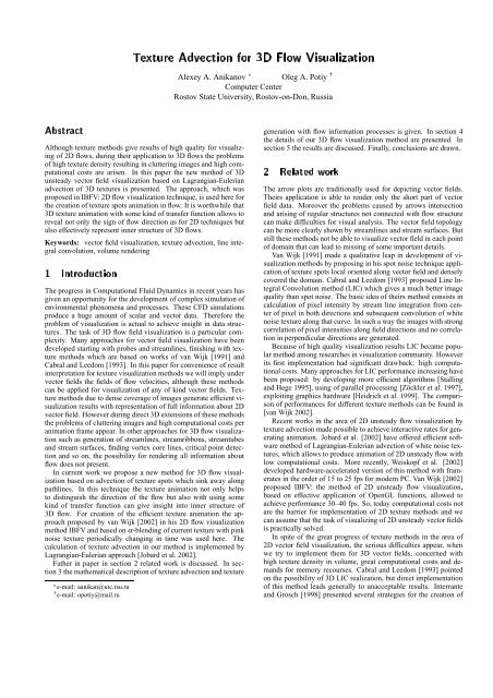
Texture Advection for 3D Flow Visualization

×ØÖ Ø
ÌÜØÙÖ Ú ØÓÒ ÓÖ ÐÓÛ Î×ÙÐÞØÓÒ
Although texture methods give results of high quality for visualizing
of 2D flows, during their application to 3D flows the problems
of high texture density resulting in cluttering images and high computational
costs are arisen. In this paper the new method of 3D
unsteady vector field visualization based on Lagrangian-Eulerian
advection of 3D textures is presented. The approach, which was
proposed in IBFV: 2D flow visualization technique, is used here for
the creation of texture spots animation in flow. It is worthwhile that
3D texture animation with some kind of transfer function allows to
reveal not only the sign of flow direction as for 2D techniques but
also effectively represent inner structure of 3D flows.
Keywords: vector field visualization, texture advection, line integral
convolution, volume rendering
ÁÒØÖÓÙ ØÓÒ
The progress in Computational Fluid Dynamics in recent years has
given an opportunity for the development of complex simulation of
environmental phenomena and processes. These CFD simulations
produce a huge amount of scalar and vector data. Therefore the
problem of visualization is actual to achieve insight in data structures.
The task of 3D flow field visualization is a particular complexity.
Many approaches for vector field visualization have been
developed starting with probes and streamlines, finishing with texture
methods which are based on works of van Wijk [1991] and
Cabral and Leedom [1993]. In this paper for convenience of result
interpretation for texture visualization methods we will imply under
vector fields the fields of flow velocities, although these methods
can be applied for visualization of any of kind vector fields. Texture
methods due to dense coverage of images generate efficient visualization
results with representation of full information about 2D
vector field. However during direct 3D extensions of these methods
the problems of cluttering images and high computational costs per
animation frame appear. In other approaches for 3D flow visualization
such as generation of streamlines, streamribbons, streamtubes
and stream surfaces, finding vortex core lines, critical point detection
and so on, the possibility for rendering all information about
flow does not present.
In current work we propose a new method for 3D flow visualization
based on advection of texture spots which sink away along
pathlines. In this technique the texture animation not only helps
to distinguish the direction of the flow but also with using some
kind of transfer function can give insight into inner structure of
3D flow. For creation of the efficient texture animation the approach
proposed by van Wijk [2002] in his 2D flow visualization
method IBFV and based on α-blending of current texture with pink
noise texture periodically changing in time was used here. The
calculation of texture advection in our method is implemented by
Lagrangian-Eulerian approach [Jobard et al. 2002].
Father in paper in section 2 related work is discussed. In section
3 the mathematical description of texture advection and texture
£ e-mail: aanikan@uic.rsu.ru
† e-mail: opotiy@mail.ru
Alexey A. Anikanov £ Oleg A. Potiy †
Computer Center
Rostov State University, Rostov-on-Don, Russia
generation with flow information processes is given. In section 4
the details of our 3D flow visualization method are presented. In
section 5 the results are discussed. Finally, conclusions are drawn.
ÊÐØ ÛÓÖ
The arrow plots are traditionally used for depicting vector fields.
Theirs application is able to render only the short part of vector
field data. Moreover the problems caused by arrows intersection
and arising of regular structures not connected with flow structure
can make difficulties for visual analysis. The vector field topology
can be more clearly shown by streamlines and stream surfaces. But
still these methods not be able to visualize vector field in each point
of domain that can lead to missing of some important details.
Van Wijk [1991] made a qualitative leap in development of visualization
methods by proposing in his spot noise technique application
of texture spots local oriented along vector field and densely
covered the domain. Cabral and Leedom [1993] proposed Line Integral
Convolution method (LIC) which gives a much better image
quality than spot noise. The basic idea of theirs method consists in
calculation of pixel intensity by stream line integration from center
of pixel in both directions and subsequent convolution of white
noise texture along that curve. In such a way the images with strong
correlation of pixel intensities along field directions and no correlation
in perpendicular directions are generated.
Because of high quality visualization results LIC became popular
method among researches in visualization community. However
its first implementation had significant drawback: high computational
costs. Many approaches for LIC performance increasing have
been proposed: by developing more efficient algorithms [Stalling
and Hege 1995], using of parallel processing [Zöckler et al. 1997],
exploiting graphics hardware [Heidrich et al. 1999]. The comparison
of performances for different texture methods can be found in
[van Wijk 2002].
Recent works in the area of 2D unsteady flow visualization by
texture advection made possible to achieve interactive rates for generating
animation. Jobard et al. [2002] have offered efficient software
method of Lagrangian-Eulerian advection of white noise textures,
which allows to produce animation of 2D unsteady flow with
low computational costs. More recently, Weiskopf et al. [2002]
developed hardware-accelerated version of this method with framerates
in the order of 15 to 25 fps for modern PC. Van Wijk [2002]
proposed IBFV: the method of 2D unsteady flow visualization,
based on effective application of OpenGL functions, allowed to
achieve performance 30–40 fps. So, today computational costs not
are the barrier for implementation of 2D texture methods and we
can assume that the task of visualizing of 2D unsteady vector fields
is practically solved.
In spite of the great progress of texture methods in the area of
2D vector field visualization, the serious difficulties appear, when
we try to implement them for 3D vector fields, concerned with
high texture density in volume, great computational costs and demands
for memory recourses. Cabral and Leedom [1993] pointed
on the possibility of 3D LIC realization, but direct implementation
of this method leads generally to unacceptable results. Interrante
and Grosch [1998] presented several strategies for the creation of

efficient visualization by 3D LIC, including defining an appropriate
input 3D texture, highlighting regions of interest, clarifying relative
depths of the texture elements by application of halo that fully
encloses each streamline. Rezk-Salama et al. [1999] suggested interactive
functionality for investigating of 3D LIC texture such as
transfer function control and volume clipping mechanisms. Furthermore
they proposed several approaches for animating 3D LIC
texture with low computational costs. However in theirs approach
the animation is created by changing volume boundaries rather than
moving of texture elements that looks not so naturally like in 2D
texture methods. Recently one more 3D LIC texture rendering
method [Chen et al. 2002] was suggested based on superposition
of current texture with opacity map, where voxel opacity is proportional
the distances from given voxel to critical points and vortex
core lines, as well as implementation of 3D streamline illumination
model [Zöckler et al. 1996] for volume rendering. This method
allows to effectively highlight the 3D vector field structure in the
regions of vortexes and near critical points. However frequently the
researcher needs to investigate the vector field without these features,
e.g. the field of flows around some object.
State of the art 3D LIC have restricted the case of steady vector
field visualization. This limitation is caused by streamlines integration
which generally are changed greatly during even small
field changes. Moreover, in the given approach the difficulties with
creation of texture spots animation along streamlines concerning
great computational costs for one frame calculation appear. The implementation
of texture advection is more convenient for 3D flows
that allows to create efficiently unsteady field visualization and to
generate texture spots animation. One of the first 3D texture advection
methods is suggested in [Kao et al. 2001]. In the given
work for the creation of animation the advection of semitransparent
spherical textures distributed in volume was used. Weiskopf et al.
[2001] developed hardware-accelerated texture advection method
for nVIDIA GeForce 3 graphics cards. They used the texture advection
for generating of animation of particles in flow as well as
showing short pathlines by combining the four last frames.
It is worthwhile to note that the methods with using of 3D textures
are the only at the beginning of evolution and also much work
can be made for the achievement of qualitative results.
ÌÜØÙÖ Ú ØÓÒ
In this section we briefly describe the Lagrangian-Eulerian approach
for texture advection suggested in [Jobard et al. 2002] for
purpose of 2D flow visualization. This approach does not have limitation
on texture dimension that gives us an opportunity for its effective
implementation for the creation of 3D texture animation.
Also we will give a description of technique for generation of textures
with flow information. The given technique was proposed in
the work [van Wijk 2002] and is based on blending of background
changing in time noise texture with last advected texture. The combination
of these two approaches, which were used before for building
of 2D flow interactive visualization, allows us to develop an effective
method for calculation of sequence of 3D textures, which
can be used for visualizing of 3D vector field structure by theirs
rendering and animation.
ÄÖÒÒ ÙÐÖÒ ÔÔÖÓ
Consider an unsteady vector field f xt : E ¢J R n defined on an
open set E of Euclidean space R n and a time interval J t 0 t end ℄.
In this paper we are interested in case n 3. Let for some point
of time t 0 J the 3D texture T xt 0 , x E is given. Our task is
to define the way for finding of texture T xt , which is a result of
advection of initial texture T xt 0 until time t J, t t 0 ,inflow
determined by vector field f xt .
For solving the task of texture advection it is convenient to consider
a set of advected particles s i densely covered the domain E.
Then we can consider the advection process for the texture T xt
as an evolution process of collection of particles s i , for each of
theirs the property T s i is assigned, which equals to the value of
texture T xt at the point of location of the particle s i at the time
t 0 . For point of time t J each point x E is connected with some
particle from s i that located at given point. We label this particle
as s xt . The invariant of property T along particle pathline can be
expressed by the following equation
∂T s xt
f xt ∇T s xt 0 (1)
∂t
The given equation can be regarded from two points of view. On the
one hand, it describes the process of advection of texture T xt ,
which can be thought as some scalar field that is known for each
point of time in any point of the domain E. In such consideration
particles lose their identity. The approach of direct solving of the
equation (1) was called Eulerian. Other point of view on the given
equation is connected with Lagrangian approach that is based on
computing of the trajectory of each particle in the flow separately.
The trajectory or pathline of particle s labeled by ps t is determined
by the equation
dps t
dt f pst (2)
The basic idea of the Lagrangian-Eulerian advection technique
[Jobard et al. 2002] consists in combination of the two above approaches.
Namely, for calculation of the sequence of advected
textures during each iteration, coordinates of the particles densely
covered the texture domain are updated with a Lagrangian scheme
whereas the advection of the particle property is achieved with an
Eulerian method. Let us consider the description of this technique
in more detail.
For computing of the advection of texture T xt during time
interval h the coordinates of each voxel pvox 0 of given texture are
integrated backward in time with step h. By integration of the
equation (2) we obtain
pvox h pvox 0
0
h
f p vox τ t τ dτ (3)
To find the values of texture T xt , for each voxel the value of
texture T xt h is assigned which is given from the point appropriated
to the coordinates of the voxel that was integrated with step
h. Namely,
T pvox h t h pvox h E
T pvox 0 t
(4)
sptci f ied value pvox h E
Van Wijk [2002] showed that in practice in case of pvox h E
it is convenient to assign the value T pvox 0 t h , i.e. to remain
the value of previous texture.
In such a way, by repeating the given process of coordinate integration
and particle property advection, we obtain a set of 3D
textures which represent the advection of the initial texture T xt 0
in the flow with step in time equals h.
ÖØÓÒ Ó ØÜØÙÖ ÛØ ­ÓÛ ÒÓÖÑØÓÒ
Lagrangian-Eulerian advection method gives the possibility for efficient
calculation of the sequence of textures, the animation of them
can represent the vector field structure. However, the separate frame
of such animation generally does not contain the information about

the field. It is more efficient for visualization purposes to use the sequence
of textures so that each separate texture from it could show
the vector field structure. Van Wijk [2002] suggested an effective
method for generation of such textures, called IBFV (Image Based
Flow Visualization) and based on α-blending of advected texture
with background texture which is changing in time. He used the
given method for creation of 2D texture animation and he computed
the texture advection by mapping some mesh onto 2D image,
forward integrating of mesh vertexes along pathlines and mapping
distorted cells of mesh into OpenGL framebuffer. Such an approach
for texture advection allows to achieve high performance due to
hardware acceleration, but it is restricted by only 2D cases. We will
use Lagrangian-Eulerian advection that will allow us to develop the
approach for 3D vector field visualization.
Let us proceed to description of the way for texture sequence
generation by IBFV method. We label by p k the sequence of
points which are the discrete approximation of the solution of equation
(2), where k N and t kh. Figure 1 shows the pipeline
of given method. At first the advection of texture T xk is re-
Figure 1: Texture sequence generation.
alized, then α-blending of given texture with background texture
G xk 1 is executed. The final texture is stored in output sequence
of textures and is passed to input of next iteration. Let us
show, that given process generates the textures with flow information.
Taking into account the formula (4) we can rewrite given process
in the following form
T p k k 1 α T p k 1 k 1 αG p k k (5)
where α 01℄. By eliminating the recurrency in (5) we obtain
T pk k 1 α k k 1
T p0 0 α ∑ 1 α
i0
i G pk i k i (6)
Since for large k the initial texture T p0 0 is tacking away by the
flow, then we can ignore the first term in (6). Finally we have
k 1
T pk k α ∑ 1 α
i0
i G pk i k i (7)
In such a way the value of the texture T at point pk is given by line
integral convolution along the pathline passed through given point,
where convolution is calculated not for single texture as in state
of the art LIC, but for texture sequence G xi . The convolution
filter kernel is defined by expression α 1 α i and is exponentially
decayed. As a result for appropriate set of background textures G
and the value of parameter α the textures T will consist the flow
information.
­ÓÛ Ú×ÙÐÞØÓÒ
In this section the detail description of the method for 3D vector
field visualization by texture advection is given. The way for selection
of the sequence of background textures, which significantly
influence on the visualization quality, is presented. Hardwareaccelerated
volume rendering of 3D textures is described.
ÌÝÔ Ó ÖÓÙÒ ØÜØÙÖ
The greatest part of texture methods of visualization implement
white noise texture as a basic texture, which further is convoluted
or undergo other treatment. Such approach allows to create for 2D
case the fine grain textures, which present flow information at every
point. The texture animation in these methods is used for resolve
the ambiguity in sign of vector field direction. In 3D case fine grain
textures cover the volume too densely for some types of vector field,
and consequently after volume rendering the problem with interpretation
of inner structure of vector field appears. In our method as
in IBFV technique for the purpose of more effective adjusting of
visualization process the scale parameter for the texture spots in
background textures is used.
We found that large scale spot noise is useful for 2D flow visualization
too. For example, figure 2 shows the animation frames obtained
from Hill’s vortex visualization by IBFV with application of
background texture spots with different scale. For generating of the
right image the white noise texture with size 16 ¢16 was increased
in 32 times and was used as background texture (the texture values
at intermediate pixels was bilinear interpolated ). For left image we
used the increasing of white noise texture with size 128 ¢128 in 4
times. Both images have the size 512 ¢ 512 pixels. The left image
Figure 2: Frames of Hill’s vortex visualization by IBFV with application
of background texture spots with different scale.
is more detailed than the right one and it allows to show the flow
direction at every point of domain. The right image loses such high
self-descriptiveness, but this shortcoming is successively compensated
by animation presented the motion direction. Moreover, on
the right image vector field is shown in simplified manner and visualization
results have the natural appearance of smoke advection.
We used direct 3D extension of method proposed in [van Wijk
2002] for generating of the sequence of 3D textures G xi , blended
in flow according equation (7). Namely, for calculation of texture
G xk from the sequence of M textures the regular mesh lay on
texture domain, which is more rough than the mesh of voxel vertexes.
The texture values at vertexes of that mesh is computed by
the following formula
G p node k w kM φ p node mod 1 (8)
Here w t is some function determined for t 01℄, φ is a random
phase, p node is a vertex point of mesh. The values of texture G xk
in voxels with location unmatched with p node are computed by trilinear
interpolation. The size of cells of superimposed mesh defines
the scale parameter for texture spots. In such a way we obtain the
texture sequence, every member of which is an increased and trilinear
interpolated texture of white noise. The function w t determines
the law of flashing of spots in noise whereas the sequence of
M textures defines the changing period for initial texture G x0 .In

this work we used step function w t :
1
w t
0
t
t
005
051℄
(9)
Physical meaning of the blending of sequence of textures G xi
(0 i M) during advection process consists in injection of texture
spots into the flow during period of time defined by the value of M.
Figure 3 shows an example of 3D spot noise texture. The extension
of white noise with size 8 3 onto texture with size 128 3 is used here.
Light colors are made transparent.
ÐÓÖØÑ
Figure 3: Large scale spot noise texture.
Let us proceed to description of the algorithm of calculation of the
sequence of 3D textures, which present the texture spot advection
in the flow. At the beginning we want to specify the selection of the
numerical method for voxel coordinate integration during computing
of texture advection. In this work for finding the point pvox h
in (3) we used simple approximation by Euler integration method:
pvox t h pvox t h f p vox t t (10)
The implementation of such rough approximation is acceptable in
case of application of small step h (with value of h f p vox 0 0 in
the order of 1–2 voxels). More accurate approximation is unpractical
due to a huge amount of calculations for 3D texture advection.
The process of calculation begins from initialization of sequence
of M background textures G xi as described above in section 4.1.
Further, the first texture T x0 is selected to be equal to G x0
and displayed by volume rendering or saved in memory separated
for sequence of textures T xi .
Let us assume that T xk was already calculated. Then the
following operations need to implement for computing the texture
T xk 1 .
The coordinated of each voxel of texture T xk 1 is integrated
with time step h by formula (10) with the value of vector field f at
the point of time k 1. The values of texture T xk 1 at centers
of voxels is computed by the formula
T pvox t k
T pvox t h k
1
T pvox t k
pvox t h E
pvox t h E
(11)
It is important to note that for points, which are not equal to voxel
centers, the values of texture T pvox t h k are calculated by trilinear
interpolation. So the advection T xk T xk 1 is implemented.
Then the values of T xk 1 are blended with the
values of the background texture G x k 1 mod M by the formula
T xk 1 1 α T xk 1 αG xk 1 (12)
whereupon the texture T xk 1 is displayed or saved in memory
and passed to input of next iteration.
The animation is generated during rendering of sequence of textures
T xk , which shows the motion of texture spots in 3D flow,
and its separate frame will be able to present the structure of the
visualized vector field for large k.
ÊÒÖÒ
For display of 3D textures we implemented hardware-accelerated
volume rendering [Blythe and McReynolds 2000]. The practical
realization of the given method is restricted to graphics hardware
with support of OpenGL 1.2 and higher. (OpenGL 1.1 does not
include the support of 3D textures.)
Figure 4: Clipping of bounding box of the volume by equidistant
slices paraller to the image plane.
The principal idea of the hardware-accelerated volume rendering
consists in follows. Multiple equidistant planes parallel to the image
plane are clipped against the bounding box of the volume (see
Figure 4). The appropriate 3D texture coordinates are assigned to
vertexes of polygons generated by clipping that allows to exploit
the hardware during rasterization for reconstruction of the texture
samples by trilinearly interpolating within the volume. For final image
generation the successive α-blending of the textured polygons
back-to-front onto the image plane is implemented. Let us note that
adjustment of the transfer function must be taken for achievement
3D texture images of good quality.
The application of hardware-accelerated volume rendering described
above gives an opportunity for the generation of interactive
rotation of textured volume. It is helpful for understanding of the
inner structure of 3D flow.
Ê×ÙÐØ×
Figures 5 and 6 show the frames of animation of the 3D texture
advection process computed for the case of planar sinusoid flow.
The texture size is 128 3 for both textures. For generation of Figure
5 the textures created by extension of white noise texture with size
16 3 were used as background textures. The white noise texture with
size 128 3 was used for the creation of image shown on the Figure
6. The 3D texture animation results can be found on web-page:
http://public.uic.rsu.ru/aanikan/3dtexadvection.htm . The texture
spot motion along pathlines not only helps for showing the sign of

flow direction, but also assists us in perception of 3D vector field
inner structure.
Figure 5: The animation frame for planar sinusoid flow with application
of extension in 8 times white noise texture of size 16 3 as the
background texture.
The main difficulty in application of suggested method consists
in optimal selection of visualization parameters. The adjusting of
the following basic parameters is possible here: α used for 3D
texture blending, has effect on fading degree of texture spots; M
is number of background patterns, defines flashing period for texture
spots and consequently their length in 3D texture volume; spot
noise scale determined by white noise extension degree; transfer
function. Each of these parameters has a great influence on the visualization
result. Since at present for computing of advection of
128 3 texture by suggested technique the time of 1 minute is spent
on PC (Pentium4 1.5Gb, RAM 256Mb), then in practice the adjusting
of the given parameters is difficult. Therefore the development
of hardware-accelerated texture advection and α-blending is actual.
Figure 6: The animation frame for planar sinusoid flow with application
of white noise texture of size 128 3 as the background texture.
ÓÒ ÐÙ×ÓÒ
In this work the new technique for 3D unsteady vector field visualization
by Lagrangian-Eulerian advection of 3D textures is suggested.
For the creation of animation of texture spots in flow the
approach proposed by van Wijk in his IBFV technique based on αblending
of advected texture with background periodically changed
texture is used. Our method is able to compute the 3D texture sequence,
which is used for the creation of interactive animation by
hardware-accelerated volume rendering for graphics hardware with
3D texture support.
The following directions can be selected for the future researches.
The development of the hardware-accelerated methods
for advection and α-blending of 3D textures can assist researchers
in creation of interactive 3D flow visualization methods by texture
advection. The application of special illumination models and ray
tracing can lead to significant increase of visualization quality.
ÒÓÛÐÑÒØ×
We acknowledge the support of Russian Foundation for Basic Research
under grant 01–01–00077, Ministry of Industry, Science and
Technology of the Russian Federation under grant 37.011.11.0010,
as well as the support of the President of the Russian Federation
under grant MK–1149.2003.01.
ÊÖÒ ×
BLYTHE, D., AND MCREYNOLDS, T. 2000. Advanced graphics programming
techniques using opengl. In SIGGRAPH 2000 Course 32.
CABRAL, B., AND LEEDOM, L. C. 1993. Imaging vector fields using line
integral convolution. In Proceedings of ACM SIGGRAPH 93, Computer
Graphics Proceedings, Annual Conference Series, ACM, 263–272.
CHEN, L., FUJISHIRO,I., AND SUZUKI, Y. 2002. Comprehensible volume
lic rendering based on 3d significance map. In Proceeding of SPIE VDA
’02, 142–153.
HEIDRICH,W.,WESTERMANN, R., SEIDEL, H.-P., AND ERTL, T. 1999.
Applications of pixel textures in visualization and realistic image synthesis.
In ACM Symposium on Interactive 3D Graphics, 127–134.
JOBARD, B., ERLEBACHER, G., AND HUSSAINI, M. Y. 2002.
Lagrangian-eulerian advection of noise and dye textures for unsteady
flow visualization. IEEE Transactions on Visualization and Computer
Graphics 8, 3, 211–222.
KAO, D., ZHANG, B., KIM, K., AND PANG, A. 2001. 3d flow visualization
using texture advection. In IASTED International Conference on
Computer Graphics and Imaging ’01, 252–257.
REZK-SALAMA, C., HASTREITER,P.,TEITZEL, C., AND ERTL, T. 1999.
Interactive exploration of volume line integral convolution based on 3dtexture
mapping. In Proceedings IEEE Visualization ’99, 233–240.
STALLING, D., AND HEGE, H.-C. 1995. Fast and resolution independent
line integral convolution. In Proceedings of ACM SIGGRAPH 95, Computer
Graphics Proceedings, Annual Conference Series, ACM, 249–256.
VAN WIJK, J. J. 1991. Spot noise: Texture synthesis for data visualization.
In Computer Graphics (Proceedings of ACM SIGGRAPH 91), vol. 25,
ACM, 309–318.
VAN WIJK, J. J. 2002. Image based flow visualization. ACM Transactions
on Graphics 21, 3, 745–754.
WEISKOPF, D., HOPF, M., AND ERTL, T. 2001. Hardware-accelerated
visualization of time-varying 2d and 3d vector fields by texture advection
via programmable per-pixel operations. In Vision, Modeling, and
Visualization VMV ’01 Conference Proceedings, 439–446.

WEISKOPF, D., ERLEBACHER, G., HOPF, M., AND ERTL, T. 2002.
Hardware-accelerated lagrangian-eulerian texture advection for 2d flow
visualization. In Vision, Modeling, and Visualization VMV ’02 Conference
Proceedings, G. Greiner, H. Niemann, T. Ertl, B. Girod, and H.-P.
Seidel, Eds., 77–84.
ZÖCKLER, M., STALLING, D., AND HEGE, H.-C. 1996. Interactive visualization
of 3d-vector fields using illuminated streamlines. In Proceedings
IEEE Visualization ’96, 107–114.
ZÖCKLER, M., STALLING, D., AND HEGE, H.-C. 1997. Parallel line
integral convolution. Parallel Computing 23, 7, 975–989.
ÓÙØ Ø ÙØÓÖ
Alexey A. Anikanov: PhD equivalent, a research associate at Laboratory
of Computing Experiment on Supercomputer, Computer
Center of Rostov State University. He is an alumni of Physics Department
of Moscow State University. He received a PhD equivalent
from Rostov State University in 2001. The theme of the PhD
thesis was: Output Data Visualization and Animation for Computer
Models of Watershed Ecosystems. He is a developer of visualization
software: VisAEffect. The address of his home page:
http://public.uic.rsu.ru/aanikan .
Oleg A. Potiy is a post-graduate student of Computer Center of
Rostov State University. He received master’s degree from Rostov
State University in 2002. The theme of the master’s thesis was:
Application of Subdivision Surfaces for Stream Surface Rendering.