An Optical Demonstration of Fractal Geometry - Materials Science ...
An Optical Demonstration of Fractal Geometry - Materials Science ...
An Optical Demonstration of Fractal Geometry - Materials Science ...

Create successful ePaper yourself
Turn your PDF publications into a flip-book with our unique Google optimized e-Paper software.
!<br />
!<br />
!<br />
!<br />
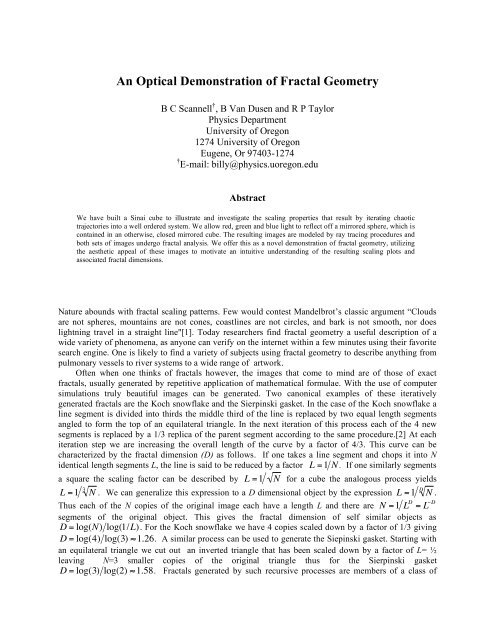
<strong>An</strong> <strong>Optical</strong> <strong>Demonstration</strong> <strong>of</strong> <strong>Fractal</strong> <strong>Geometry</strong><br />
B C Scannell † , B Van Dusen and R P Taylor<br />
Physics Department<br />
University <strong>of</strong> Oregon<br />
1274 University <strong>of</strong> Oregon<br />
Eugene, Or 97403-1274<br />
† E-mail: billy@physics.uoregon.edu<br />
Abstract<br />
We have built a Sinai cube to illustrate and investigate the scaling properties that result by iterating chaotic<br />
trajectories into a well ordered system. We allow red, green and blue light to reflect <strong>of</strong>f a mirrored sphere, which is<br />
contained in an otherwise, closed mirrored cube. The resulting images are modeled by ray tracing procedures and<br />
both sets <strong>of</strong> images undergo fractal analysis. We <strong>of</strong>fer this as a novel demonstration <strong>of</strong> fractal geometry, utilizing<br />
the aesthetic appeal <strong>of</strong> these images to motivate an intuitive understanding <strong>of</strong> the resulting scaling plots and<br />
associated fractal dimensions.<br />
Nature abounds with fractal scaling patterns. Few would contest Mandelbrot’s classic argument “Clouds<br />
are not spheres, mountains are not cones, coastlines are not circles, and bark is not smooth, nor does<br />
lightning travel in a straight line"[1]. Today researchers find fractal geometry a useful description <strong>of</strong> a<br />
wide variety <strong>of</strong> phenomena, as anyone can verify on the internet within a few minutes using their favorite<br />
search engine. One is likely to find a variety <strong>of</strong> subjects using fractal geometry to describe anything from<br />
pulmonary vessels to river systems to a wide range <strong>of</strong> artwork.<br />
Often when one thinks <strong>of</strong> fractals however, the images that come to mind are <strong>of</strong> those <strong>of</strong> exact<br />
fractals, usually generated by repetitive application <strong>of</strong> mathematical formulae. With the use <strong>of</strong> computer<br />
simulations truly beautiful images can be generated. Two canonical examples <strong>of</strong> these iteratively<br />
generated fractals are the Koch snowflake and the Sierpinski gasket. In the case <strong>of</strong> the Koch snowflake a<br />
line segment is divided into thirds the middle third <strong>of</strong> the line is replaced by two equal length segments<br />
angled to form the top <strong>of</strong> an equilateral triangle. In the next iteration <strong>of</strong> this process each <strong>of</strong> the 4 new<br />
segments is replaced by a 1/3 replica <strong>of</strong> the parent segment according to the same procedure.[2] At each<br />
iteration step we are increasing the overall length <strong>of</strong> the curve by a factor <strong>of</strong> 4/3. This curve can be<br />
characterized by the fractal dimension (D) as follows. If one takes a line segment and chops it into N<br />
identical length segments L, the line is said to be reduced by a factor L =1 N . If one similarly segments<br />
a square the scaling factor can be described by L =1 N for a cube the analogous process yields<br />
3<br />
D<br />
L =1 N . We can generalize this expression to a D dimensional object by the expression L =1 N .<br />
Thus each <strong>of</strong> the N copies <strong>of</strong> the original image each have ! a length L and there are N =1 L<br />
!<br />
!<br />
!<br />
D = L "D<br />
segments <strong>of</strong> the original object. This gives the fractal dimension <strong>of</strong> self similar objects as<br />
D = log(N) log(1/L). For the Koch snowflake we have 4 copies scaled down by a factor <strong>of</strong> 1/3 giving<br />
D = log(4) log(3) "1.26. A similar process can be used to generate the Siepinski gasket. Starting with<br />
an equilateral triangle we cut out an inverted triangle that has been scaled down by a factor <strong>of</strong> L= ½<br />
leaving N=3 smaller copies <strong>of</strong> the original triangle thus for the Sierpinski gasket<br />
D = log(3) log(2) "1.58. <strong>Fractal</strong>s generated by such recursive processes are members <strong>of</strong> a class <strong>of</strong>
fractals known as Iterated Function Systems (ITS). Figure 1 shows the original image followed by the<br />
first two iterations <strong>of</strong> each <strong>of</strong> these processes.<br />
Figure 1: The starting point and first two iterations <strong>of</strong> the generation processes <strong>of</strong> the (top) Koch<br />
snowflake and (bottom) Sierpinski gasket.<br />
<strong>An</strong> intuitive feel for what D actually characterizes can be rather difficult to grasp. One possible<br />
interpretation that works well for coastlines or curves such as the Koch snowflake is that D can be viewed<br />
as a measure <strong>of</strong> the crinkliness <strong>of</strong> the curve or its lack <strong>of</strong> smoothness. This interpretation serves well for<br />
as a description <strong>of</strong> D provided that it is the edges <strong>of</strong> a pattern that result in the fractal scaling. But such a<br />
description is lacking for an intuitive feel to filled patterns such as the Sierpinski gasket.<br />
While analytic determination <strong>of</strong> D is fitting or at least possible for fractals generated via IFS,<br />
difficulty arises when one encounters a fractal produced by natural processes. To estimate D for these<br />
processes typically one employs the box counting procedure. In this procedure one superimposes a grid <strong>of</strong><br />
boxes <strong>of</strong> length L on a two dimensional image <strong>of</strong> the object in question and counts the number <strong>of</strong> boxes<br />
that contain a piece <strong>of</strong> the object N. The box size is then decreased and the counting <strong>of</strong> filled boxes is<br />
repeated until a suitably large range <strong>of</strong> L has been spanned. One can then produce a scaling plot in which<br />
log(N) is plotted as a function <strong>of</strong> log(1/L) and D is determined by the slope <strong>of</strong> the curve. In this scenario<br />
an object is said to be fractal if 1< D < 2, provided that the expression N " L<br />
!<br />
!<br />
#D holds for at least 1 order<br />
<strong>of</strong> magnitude.<br />
Figure 2 shows an example <strong>of</strong> the scaling plots <strong>of</strong> the Sierpinski gasket and the Koch curve. When<br />
plotted in this manner it is convenient to interpret the log(1/L) as describing the box size as ranging from<br />
coarse scaling in which just a few boxes span the image to fine scaling where the number <strong>of</strong> boxes<br />
necessary to span the image becomes quite large.<br />
In this way one can picture the value <strong>of</strong> D as a measure <strong>of</strong> the fine scale structure <strong>of</strong> the pattern. We<br />
see in Figure 2 that the Koch curve (bottom inset) does not seem to have as much complexity at fine<br />
scales as the Sierpinski gasket (top inset). The fact that the Sierpinski gasket fills more fine scale boxes is<br />
readily evident in that N is larger for the Sierpinski gasket than the Koch curve at the fine scale end <strong>of</strong> the<br />
plot while both curves are anchored at the same coarse scale values. In some sense this implies that one<br />
can view D to be a measure <strong>of</strong> the ability <strong>of</strong> the object to occupy space at fine scales.
Figure 2: Scaling plots generated by the analytic value <strong>of</strong> the fractal dimension <strong>of</strong> the Sierpinsk<br />
gasket (top scaling plot with D =1.58 and inset) and the Koch snowflake (bottom scaling plot with D=<br />
1.26 and inset).<br />
For the past few years work in our lab has focused on fractal scaling properties <strong>of</strong> conductance<br />
fluctuations in semiconductor billiards. In 1996 Ketzmeric published a paper illustrating that the mixed<br />
(chaotic and regular) phase space <strong>of</strong> chaotic systems would generate fractal trajectories.[3] He went on to<br />
predict that the conductance fluctuations <strong>of</strong> semiconductor nanostructures would exhibit this fractal<br />
scaling. In 1997 Taylor et al. reported the first experimental observation <strong>of</strong> self similarity in the so called<br />
Sinai billiard.[4] Figure 3 illustrates the transition from regular to chaotic dynamics that emerge as a<br />
result <strong>of</strong> altering device geometry.<br />
Figure 3: a) A square billiard exhibits regular dynamic, trajectories with similar initial conditions<br />
do not diverge. B) Introducing a circular scatterer (Sinai diffuser) creates trajectories that are<br />
exponentially sensitive to their initial conditions, thus introducing chaos to the system.<br />
A few years ago Marlow et al. presented a unified view <strong>of</strong> these conductance fluctuations based on a<br />
comprehensive comparison <strong>of</strong> several device regimes, showing that these fractal scaling patterns in the<br />
conductance fluctuations were not dependent on the device geometry or scattering regime properties that<br />
Ketzmeric’s proposal did not explain.[5] We <strong>of</strong>fered a unified model, proposing that the electrostatic<br />
influence <strong>of</strong> remote ionized regions acted as Sinai diffusers in the devices. In essence, the fractal patterns<br />
resulted from the device walls allowing repeated reflection <strong>of</strong>f <strong>of</strong> the diffusers, iterated chaos akin to the<br />
IFS mentioned above.<br />
Coupling this idea with our lab’s dedication to physics education, we set out to develop a simple<br />
demonstration <strong>of</strong> this phenomenon suitable for use in the classroom. Intrigued by the apparatus described
y Sweet et al.,[6] we first built a light scattering system consisting <strong>of</strong> four reflective spheres stacked in a<br />
pyramid formation. Replicating Sweet’s experiment we illuminate the top three openings created by the<br />
stacked configuration with colored light. The fourth (bottom) opening is used to capture an image <strong>of</strong> the<br />
pattern created by the iterated reflections. This apparatus displays the properties <strong>of</strong> Sinai diffusers in the<br />
absence <strong>of</strong> wall boundaries. To investigate the influence <strong>of</strong> the wall on this sort <strong>of</strong> system we built a Sinai<br />
cube. This also had the advantage <strong>of</strong> being a classical analog <strong>of</strong> Sinai diffuser model <strong>of</strong> our electron<br />
billiards. Using front surface mirrors we constructed a set <strong>of</strong> cubes with openings at the upper corners.<br />
We suspend a reflective sphere from the top mirror creating the Sinai cube. Three <strong>of</strong> the top corners are<br />
illuminated with colored light, and in the fourth corner we place a camera to capture the image created by<br />
the lights repeated reflection <strong>of</strong>f <strong>of</strong> the Sinai diffuser. In Figure 4 we show these apparatuses.<br />
Figure 4: The two experimental apparatuses are pictured above. On the left is a recreation <strong>of</strong> the<br />
laboratory model presented by Sweet et al. On the right is our Sinai cube shown here without the top<br />
mirror in place and with a Sinai diffuser whose diameter is approximately equal to the wall width.<br />
We use ray tracing techniques[7] to model both the stacked sphere and Sinai cube images with good<br />
results. Figure 5 shows the image obtained from the bottom opening <strong>of</strong> the stacked sphere configuration<br />
(top) as well as the ray tracing model (bottom). In Figure 6 we show the experimental (top) and modeled<br />
(bottom) Sinai cube in which the diffuser diameter is roughly 1/3 the wall width. A box counting analysis<br />
was performed on both sets <strong>of</strong> images with good agreement with the values reported by Sweet et al. for<br />
the stacked spheres (D= 1.6) and good agreement between the experimental and modeled images <strong>of</strong> the<br />
Sinai cube.<br />
Taking a step back and regarding D in terms <strong>of</strong> the fine scale space filling interpretation, we are<br />
observe that the resulting D values are in line with this description as depicted in Figure 7 where we show<br />
the scaling plot <strong>of</strong> the 33% filled Sinai cube model and image (upper solid and dashed lines respectively).<br />
The lower solid line depictis the agreed upon value (D=1.6) <strong>of</strong> the stacked sphere configuration (lowest<br />
solid line).
Figure 5: (top) The image obtained from the bottom opening <strong>of</strong> the stacked sphere configuration and<br />
(bottom) the ray tracing model <strong>of</strong> that image.
Figure 6: (top) The image obtained from the opening <strong>of</strong> the Sinai cube and (bottom) the ray tracing<br />
model <strong>of</strong> that image.
Figure 7: Scaling plots <strong>of</strong> the images in figure 6 (upper dashed and solid lines respectively). The<br />
lower solid line depicts represents the scaling plot <strong>of</strong> the stacked sphere configuration.<br />
It is our hope that the inherent aesthetic quality <strong>of</strong> the images created by this simple demonstration as<br />
illustrated in Figure 8 can be used to motivate discussion <strong>of</strong> fractal geometry in high school and university<br />
math and physics curriculum. Study <strong>of</strong> fractal geometry <strong>of</strong>fers high school and lower division college<br />
students a rare opportunity to investigate a field in which the first people to really think and elaborate<br />
about the subject are still alive.<br />
Figure 8: The unaltered view from the empty top corner <strong>of</strong> the Sinai cube
Acknowledgements<br />
R.P. Taylor is a Cottrell Scholar <strong>of</strong> the Research Corporation. B. Van Dusen was funded for this project<br />
by the M.J. Murdock Foundation, Partners in <strong>Science</strong> program. We thank M.S. Fairbanks for many<br />
fruitful discussions.<br />
References<br />
[1] Benoit B. Mandelbrot, The <strong>Fractal</strong> <strong>Geometry</strong> <strong>of</strong> Nature, W.H. Freeman and Co., 1982.<br />
[2] Peitgen, H.O. and Saupe, D., The <strong>Science</strong> <strong>of</strong> <strong>Fractal</strong> Images, Springer-Verlag, 1988.<br />
[3] R. Ketzmerick, <strong>Fractal</strong> conductance fluctuations in generic chaotic cavities, Phys. Rev. B, Vol 54,<br />
pp.10841 1996<br />
[4] R.P.Taylor, R. Newbury, A.S. Sachrajda, Y. Feng, P.T Coleridge, C. Dettmann, Ningjia Zhu, Hong<br />
Guo, A. Delage, P.J. Kelly and Z. Wasilewski, Self –Similar Magnetoresitance <strong>of</strong> a Semiconductor Sinai<br />
Billiard, Phys. Rev . Lett. Vol. 78, pp.1952, 1997.<br />
[5] C.A. Marlow, R.P. Taylor, T.P> Martin, B.C. Scannell, H. Linke, M.S. Fairbanks, G.D. Hall, I.<br />
Shorubalko, L. Samuelson, T.M. Fromhold, C.V> Brown, B. Hackens, S> Faniel, C. Gustin, V. Bayot, X.<br />
Wallart, S. Bollaert, and A. Cappy, Unified model <strong>of</strong> fractal conductance fluctuations for diffusive and<br />
ballistic semiconductor devices, Phys. Rev. B, Vol. 73, 195318, 2006.<br />
[6] D. Sweet, E. Ott, J.A. Yorke, Topology in chaotic scattering, Nature, Vol. 399, pp315, 1999<br />
[7] Ray tracing was performed using a 3d modeling program called Cinema4D.