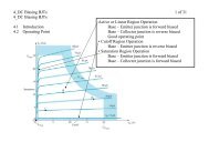
tν - MavDISK - Minnesota State University, Mankato

Notes
on
Stellar Astrophysics
by
James N. Pierce
2013

To Lee Anne Willson and George H. Bowen
© 2013 by James N. Pierce
Edition 4.0
This work is licensed under the
Creative Commons Attribution-NonCommercial-NoDerivs 3.0 Unported License.
To view a copy of the license,
visit http://creativecommons.org/licenses/by-nc-nd/3.0/deed.en_US .
ii

TABLE OF CONTENTS
PREFACE 8
CHAPTER 1: Overview 10
CHAPTER 2: Radiative Transfer 12
Radiation Terminology 12
Specific Intensity 12
Mean Intensity 13
Radiative Flux 14
Radiation Pressure 15
Radiative Energy Density 17
Radiation and Matter 18
Emission Coefficient 18
Absorption Coefficient 19
Cross Section 20
Mean Free Path 20
Nomenclature 21
The Transfer Equation for Normal Rays 21
Optical Depth 22
The Source Function 23
Solutions of the Transfer Equation 26
The Transfer Equation for Oblique Rays 30
Normal Optical Depth 31
Extended Atmospheres 32
Plane-Parallel Atmospheres 34
Solution of the Transfer Equation 35
Exponential Integrals 37
Radiative Equilibrium in the Photosphere 38
The Gray Case 40
The Eddington Approximation 41
Limb Darkening 43
The Next Step 45
CHAPTER 3: Atomic Structure 46
One-Electron Atoms 46
The Bohr Model 46
The de Broglie Wavelength 48
Electronic Transitions 51
The Quantum Mechanical Model 55
Legendre Function 60
Associated Legendre Function 60
Laguerre Polynomial 60
Associated Laguerre Polynomial 60
Quantum Numbers 61
Multi-electron Atoms 62
Pauli Exclusion Principle 62
Total Quantum Numbers 63
Electron Configurations 64
Equivalent and Non-equivalent Electrons 65
Radiative Transitions 72
iii

CHAPTER 4: Thermodynamic Equilibrium 76
Excitation 76
Boltzmann Equation 77
The Boltzmann Hotel 78
Partition Function 78
Radiative Transition Probabilities 80
Absorption/Emission Coefficients 83
Ionization 85
Saha Equation 87
The Hydrogen Atom 88
Gas-in-a-box Problem 92
Gas Mixtures 94
Multiple Ionization Stages 96
Effect on Transitions 98
CHAPTER 5: Stellar Spectra 100
Kirchhoff's Laws of Spectral Analysis 100
Line Formation 101
Column Density 102
Spectral Classification 103
Harvard System 103
Luminosity Class 106
Additional Nomenclature 107
Molecular Spectra 108
Rotational and Vibrational States 108
Band Structure 110
Notation 110
CHAPTER 6: Line Profiles 112
The Natural Line Profile 112
The Wave Equation 112
Damped Harmonic Oscillator 115
Dispersion Profile 117
Absorption Cross Sections 118
Oscillator Strength 119
Damping Constant for Radiation Damping 120
Pressure/Collisional Broadening 122
Thermal/Doppler Broadening 123
Doppler Profile 123
Voigt Function 124
Convolution 124
Hjerting Function 127
Microturbulence 127
Macroturbulence 127
Rotational Broadening 128
Equivalent Width 130
Curve of Growth 132
CHAPTER 7: Opacity Sources 133
Absorption Transitions 133
Bound-Bound Transitions 133
Bound-Free Transitions 134
iv

Free-Free Transitions 137
Scattering 138
Thomson Scattering 139
Compton Scattering 139
Rayleigh Scattering 140
CHAPTER 8: Stellar Atmospheres 142
Gas Properties 142
Particle Velocities 142
Gas Pressure 144
Mean Kinetic Energy 146
Temperature 146
Model Atmospheres 147
Hydrostatic Equilibrium 148
Ideal Gas Law 148
Mean Molecular Weight 149
Mass Fractions 150
Total Pressure 150
Equilibrium Calculations 151
The Secant Method 155
Altitude Variations 156
Effective Gravity 157
Scale Height 158
Non-equilibrium atmospheres 158
Shock Waves 158
Dynamic Scale Height 161
CHAPTER 9: Stellar Interior Models 163
Continuity of Mass 164
Hydrostatic Equilibrium 164
Equation of State 165
The Linear Model 167
Polytropes 170
Relevant Polytropes 170
The Lane-Emden Equation 172
Radius 174
Mass 174
Total Mass 175
Mean Density 175
Mass-Radius Relation 175
Central Values 176
Solutions of the Lane-Emden Equation 176
The n = 0 Solution 177
The n = 1 Solution 177
The n = 5 Solution 178
Polytropic Models 178
The Isothermal Gas Sphere 181
CHAPTER 10: Energy Generation and Transport 183
The Radiative Temperature Gradient 183
Opacity Sources 184
The Eddington Limit 185
The Adiabatic Temperature Gradient 186
Convection vs. Radiation 188
v

Energy Generation 189
Thermal Equilibrium 189
Gravitational Contraction 189
Kelvin-Helmholtz Time Scale 190
Nuclear Reactions 191
Nuclear Time Scale 192
The Proton-Proton Chain 192
The CNO Cycle 195
The Triple-Alpha Process 196
Binding Energy 197
Reaction Rates 199
Neutrinos 203
The Equations of Stellar Structure 204
CHAPTER 11: Degeneracy 207
Phase Space 207
A 2-Dimensional Example 208
Ion Degeneracy 209
Distribution Functions 209
The Degeneracy Parameter α 210
Complete Degeneracy 211
Partial Degeneracy 214
Relativistic Degeneracy 217
Relativistic, Complete Degeneracy 217
Relativistic, Partial Degeneracy 218
Fermi-Dirac Functions 219
CHAPTER 12: Stellar Synthesis 222
Star Formation 222
The Jeans Criterion 223
Free-Fall Time Scale 225
Energy Sinks 225
The Main Sequence 231
The Stellar Thermostat 232
Main Sequence Properties 232
Main Sequence Lifetimes 236
CHAPTER 13: Sequels to the Main Sequence 238
The End of the Main Sequence 238
Lower Main Sequence (Minimal and Low Mass Stars) 239
Upper Main Sequence (Medium, High, and Maximal Mass Stars) 241
Toward Helium Ignition 242
The Minimal Mass Stars 242
The Maximal and High Mass Stars 242
The Medium and Low Mass Stars 243
The Helium Flash 244
The Schönberg-Chandrasekhar Limit 247
The Hertzsprung Gap 249
Evolutionary Time Scales 249
The Approach to Carbon Burning 251
The Medium and Low Mass Stars 251
Dredge-up 252
The Maximal and High Mass Stars 252
Advanced Nucleosynthesis 253
Alpha Capture 253
vi

Neutron Capture and Beta Decay 254
Carbon Burning and Beyond 255
CHAPTER 14: Evolutionary Endpoints 258
Minimal Mass Stars 258
Medium and Low Mass Stars 258
Planetary Nebulae 260
White Dwarfs 261
High Mass Stars 265
Maximal Mass Stars 265
Supernovae 266
Neutron Stars 271
Pulsars 271
Black Holes 273
CHAPTER 15: Evolution Conclusions 275
Stellar Stories 275
Minimal Mass Stars: Mid to Late M Stars 275
Low Mass Stars: F, G, K, and Early M Stars 275
Medium Mass Stars: A Stars 276
High Mass Stars: Mid to Late B Stars 276
Maximal Mass Stars: O and Early B Stars 277
Stellar Samples 277
Time Scales 277
The Initial Mass Function 278
Selection Effects 279
Observational Data 279
Color-Magnitude Diagrams 281
APPENDIX 286
Constants 287
Solid Angle 288
REFERENCES 289
READING LIST 291
INDEX 293
ABOUT THE AUTHOR 299
vii

Pierce: Notes on Stellar Astrophysics Preface
PREFACE
This book is based primarily on lecture notes for a two-semester sequence of courses at
Minnesota State University, Mankato: Stellar Astrophysics and Stellar Structure and Evolution.
The courses, which were offered every other year, were taken by astronomy majors during their
junior or senior years; these students were expected to have completed the three-semester
Calculus sequence, Differential Equations, the General Physics sequence, the first semester of
Modern Physics, and the sophomore-level Astronomy and Astrophysics sequence. Depending on
the timing, students may or may not have been exposed to upper-level courses in Mechanics,
Electricity and Magnetism, and Quantum Mechanics. Thus, some of this material would have
been seen before, but normally not in the depth presented here. This course sequence was
intended as part of the student's preparation for graduate study in astronomy or astrophysics, and
it was expected that much of the material would be covered again at that time.
The focus of the book is on understanding the material in the courses, rather than just
memorizing it. Wherever possible, derivations of equations are presented, with sufficient
intermediate steps to lead the reader safely through the mathematical maze. In this way, the
student will comprehend why and when approximations have been made and/or certain terms or
factors have been ignored; this is important because it is necessary to understand the limits of the
equations being developed in order to properly apply them. Additionally, it is useful for the
student to be able to adapt existing equations to solve new problems.
Most of the material contained in this book has been covered by many other authors; this is
not a completely new set of basic principles, equations, derivations, and results for use in
understanding stars. Rather, it is a somewhat different organization of the standard collection of
material, based on the order in which it is presented in the two courses involved. Neither an
atmospheres/interiors split nor a principles/applications division has been used to allocate
material to the two courses or to partition the book; instead, the approach is to develop and
utilize topics as needed, such that the text flows smoothly from chapter to chapter in a logical
order. In my sequence of courses, the first semester covers Chapters 1 - 7, and the second covers
Chapters 8 - 15.
As this is a course text, an effort has been made to keep the book as readable as possible for
the student; as a result, there are relatively few references included. Where appropriate,
references are used to guide the reader to particular original sources – constants, data, models,
etc. – but for the most part the story is not liberally referenced as most of the topics have already
8

Pierce: Notes on Stellar Astrophysics Preface
been discussed in many other sources. A list of references is provided at the end of the book,
along with a reading list of books on the subject, for those needing another slant on the story.
Many of the books used as references have been out of print for some time (which has
provided much of the impetus for this project), but they are still good sources of material,
including numerous graphs, tables, and models. A number of books from the reading list have
been used as texts for these courses over the last 30 years or so, but finding a book with
satisfactory content that is written at an appropriate level and is still in print has proven to be
somewhat elusive of late. It is hoped that this text will serve as an adequate guide to basic stellar
astrophysics for some time to come.
9

Pierce: Notes on Stellar Astrophysics Chapter 1: Overview
CHAPTER 1: Overview
To many astronomers, stars are points of light in the sky; these points may have measurable
positions, velocities, magnitudes, colors, etc., but they are still just points. To the astrophysicist,
however, stars are huge balls of matter, with properties such as temperature, density, pressure,
composition, etc. that vary throughout the star and over time. This book provides an introduction
to the details of the structure, operation, and evolution of stars.
Most stars are immense balls of gaseous matter; these gases are discouraged from simply
drifting away into space by the star's gravity, which attracts the matter toward the center of the
star. At the same time, they are prevented from all piling up at the center by the pressure within
the star, which is supplied by both the matter and the radiation within the star. This pressure is
greatest at the center of the star, and we can say that the pressure gradient is generally negative.
Eq. 1.1
dP
dr
< 0
We shall find that the high pressure in a star is normally produced as a result of high
temperature, and thus the temperature gradient should also be generally negative.
Eq. 1.2
dT
dr
< 0
The high temperatures within a star serve several purposes:
• They maintain the matter in a gaseous state, usually a plasma of ions – nuclei and electrons.
• They produce radiation that ultimately escapes from the stellar surface as the star's
luminosity.
• They result in high particle velocities that smash nuclei together in the core of the star to
perform nuclear fusion, releasing energy that migrates outward towards the surface,
maintaining the high temperatures along the way.
In studying stars, astrophysicists have found it convenient to draw boundaries that divide a
star into different regions. The simplest boundary to understand is the stellar surface:
everything inside the surface is part of the stellar interior, while the stellar gases that lie above
the surface make up the stellar atmosphere. The gases of the stellar atmosphere are reasonably
transparent, or optically thin; the stellar interior is opaque, or optically thick.
10

Pierce: Notes on Stellar Astrophysics Chapter 1: Overview
Nuclear energy is released in the interiors of stars and flows outward through their interiors
and then their atmospheres. As radiation passes through the matter in both regions, photons are
emitted, absorbed, and re-emitted; the directions and/or the wavelengths of these re-emitted
photons may be altered from their original states. It is this process of radiative transfer that we
will study first.
Later chapters will deal with the structure of the atom, excitation, ionization, the
interpretation of stellar spectra, line profiles, and sources of opacity. Once these basic ideas are
in hand, they will be applied to the tasks of determining how stars are structured, how they
function, and how they form, evolve, and die.
11

Pierce: Notes on Stellar Astrophysics Chapter 2: Radiative Transfer
CHAPTER 2: Radiative Transfer
Radiation Terminology
The basic problem of radiative transfer involves the passage of radiation through matter. As
it does so, some of the radiation is absorbed, and some radiation is emitted. The rate at which
radiation is absorbed by matter will depend on the rate at which radiation is incident on the
matter – more radiation results in more absorption; the rate at which radiation is emitted will
depend only slightly on the incident radiation. The question is how the radiation changes as it
passes through matter.
Before we can find an answer, we have to decide what property of the radiation we want to
monitor. There are several possibilities, and they all begin with a quantity called the specific
intensity, I ν .
Specific Intensity
Consider rays of light of intensity I ν , passing through a surface element of area ΔA, towards
the observer at an angle θ to the normal (of the surface element), into solid angle * Δω, as shown
in Figure 2.1.
Figure 2.1: A ray of light passing through a surface element ΔA into a solid angle Δω at an
angle θ to the normal
normal
!A
!
!"
to observer
Let ΔE ν equal the amount of energy in photons with frequency in the range ν to ν + Δν,
passing through the area ΔA into solid angle Δω in a time Δt. Then the specific intensity I ν is
defined by the following:
* See Appendix: Solid Angle.
12

Pierce: Notes on Stellar Astrophysics Chapter 2: Radiative Transfer
Eq. 2.1
or
I ν ≡ lim
Δ→0
I ν ≡
ΔE ν
cosθ ΔA Δt Δν Δω
dE ν
cosθ dA dt dν dω
(Note: ΔA cos θ is the projected area.)
The limit here is a practical limit rather than a strictly mathematical limit. This means we
will shrink our Δ's down such that we are considering regions smaller than our resolving power,
but not so small as to cause problems with the uncertainty principle or other quantum
mechanical factors.
The dimensions of I ν can be obtained from the definition: in cgs units – the standard for
astronomy – E is in ergs, A is in square centimeters, t is in seconds, ν is in hertz, and ω is in
ergs
steradians, making the dimensions of Iν cm 2 . Note: The reader might observe that
-s-Hz-st
multiplication of seconds by hertz would cancel both units, thus simplifying the expression;
however, the reader should strongly resist the temptation to do this.
In general, I ν is a function of position in space, direction (of the ray), and frequency; it is a
measure of the brightness of a particular ray of a particular frequency at a particular point along
the ray. I ν can be defined for a point on a radiating surface or for a point in space (with a
specified direction).
Note that once we have taken the limit as the solid angle (Δω) goes to zero, we have a ray,
which is not divergent. This means that the energy is not being spread out over a range of angles
and diluted by distance, and hence, I ν is independent of distance from the source – I ν is constant
along a ray. The intensity of a ray of sunlight is thus constant: I ν for a point on the Sun would be
the same as measured from any planet. (Note: If this seems counter-intuitive, it is because there
is another property of radiation that does diminish with distance; stay tuned.)
Astronomers use telescopes to make stars appear brighter, but they do this not by increasing
the intensity of a ray, but rather by collecting more rays from the source. Note also that intensity
can only be measured for sources of finite angular size, such as the Sun, the Moon, or the
planets, but it cannot be measured for point sources, such as stars. Why not?
I ν depends on the angle θ between the ray to the observer and the normal to the surface at
which the intensity is measured; different rays passing through the same point but going in
different directions may have different intensities. But sometimes we do not care which
direction the rays are moving and only want to know the average value of the intensity at a point.
In this case, we can average I ν over all angles (over a sphere – over 4π) to get the mean intensity.
Mean Intensity
To find the mean intensity, J ν , we perform a weighted average. We find the specific
intensity, I ν , for each differential solid angle (dω), multiply I ν by dω, and add these products up
for the whole sphere. Then we must divide this sum by the sum of the weights – the sum of the
13

Pierce: Notes on Stellar Astrophysics Chapter 2: Radiative Transfer
differential solid angles – to obtain an average value for the intensity. Mathematically, this
becomes the following:
Eq. 2.2
J ν ≡
∫
Iνdω 4 π
=
∫ dω
4π
1
4π
∫
I ν dω
4 π
Note here that the differential solid angle can be written as dω = sin θ dθ dϕ, and the integral
in the denominator then can be easily solved:
Eq. 2.3
2π π
∫ dω = ∫ sinθ dθ dφ = ∫ sinθ dθ dφ
4 π
4π
0 0
π
∫ = 2π ∫ sinθ dθ
0
0
= 2π[cosθ] π = 4π
J ν is an intensity, as is I ν , and therefore both quantities have the same units, described above
for I ν . While I ν can vary with the direction of the ray, J ν is an average value over all angles, and
therefore it does not vary with direction. If I ν should happen to be isotropic – meaning 'direction
independent' – then I ν can be moved outside the integral to obtain the following:
Eq. 2.4
Radiative Flux
Jν = 1
∫ Iνdω =
4π 4π
1
4π Iν ∫
dω = I ν
4 π
Sometimes the question of interest is a bit different: How much energy in an arbitrary
radiation field will pass through an area ΔA in a time Δt in a frequency bandwidth Δν? (Note:
Here we have no mention of angles.) The answer to this question will be the radiative flux (or
simply, the flux) F ν , defined as follows:
Eq. 2.5
Eq. 2.6
ΔF ν =
Then taking the limit, we find
ΔEν ΔA Δt Δν =
ΔEν cosθ Δω
cosθ ΔA Δt Δν Δω
ΔEν dFν = lim ΔFν = lim
Δ→0 Δ→0 cosθ ΔA Δt Δν Δω cosθ Δω = Iν cosθ dω
From this, we find the flux to be
Eq. 2.7 Fν = ∫ I
4 π
ν cosθ dω
The units of this flux are intensity units multiplied by solid angle units, or
ergs
cm 2 -s-Hz .
Now if I ν is isotropic – a fairly common simplifying assumption – then equal amounts of
energy will pass through the area in each direction and the flux (or net flux) will be zero, as
integration confirms:
Eq. 2.8
2π
Fν = Iν ∫ cosθ dω = Iν cosθ sinθ dθ dφ = 2π Iν 4π ∫0
∫0
= π Iν [sin 2 π
θ] 0 = 0
π
14
∫
π
0
sinθ cosθ dθ

Pierce: Notes on Stellar Astrophysics Chapter 2: Radiative Transfer
In performing these integrations, the convention is to label the outward normal as θ = 0, as
shown in Figure 2.2.
Figure 2.2: Angular coordinate convention at the stellar surface
! = "/2
surface
! = 0
!
! = "
Sometimes only the outward flux (or emittance) is desired. This can be found the same as in
Equation 2.7 but integrating over only the outward hemisphere, which can be accomplished by
changing the limits of integration.
Eq. 2.9
+
Fν = ∫ Iν cosθ dω
2π
And if I ν is isotropic, the integral can proceed easily:
Eq. 2.10
+
Fν = Iν cosθ dω
2π
2π
π /2
out
in
∫ = Iν ∫ ∫ cosθ sinθ dθ dφ = 2π Iν = π Iν [sin 2 π /2
θ] 0 = π Iν
0
0
∫
π /2
0
sinθ cosθ dθ
There are some who would prefer to eliminate the factor of π that appears in the result for
Equation 2.10 (F ν + = πIν ), and this has been done by defining a quantity (F ν ≡ F ν /π) most
generally known as the astrophysical flux (see Gray (1976), Novotny (1973), Bohm-Vitense
(1989)), but also as the radiative flux (see Collins (1989)). Bowers and Deeming (1984) have the
same two quantities but reverse the notation: their flux is F ν while their astrophysical flux is F ν ,
making their linking equation F ν = πF ν . In this book, we will not use the astrophysical flux.
There are some occasions where it is useful to define a flux in the same manner as we
defined the mean intensity – as a weighted average of a quantity. In this case, the quantity to
average is the product I ν cos θ. The result is H ν – the Harvard flux or Eddington's flux.
Eq. 2.11
H ν ≡
Radiation Pressure
∫
Iν cosθ dω
4 π
=
∫ dω
4 π
1
∫ Iν cosθ dω =
4π 4π
Fν 4π
Photons exert pressure – radiation pressure, designated P ν . Radiation pressure is
responsible for the dust tails of comets, as it pushes the tiny dust particles released by the comet
15

Pierce: Notes on Stellar Astrophysics Chapter 2: Radiative Transfer
into higher orbits about the Sun. It also makes an important contribution to the pressure at very
high temperatures in stars.
Radiation pressure can be calculated for a particular intensity as follows. In general, pressure
is equal to force per unit area, with only the component of the force that is perpendicular to the
area being counted. But because force is the time derivative of momentum, pressure is then
equal to the momentum flux.
⊥ force
Eq. 2.12 pressure =
area =
d
⊥ momentum
dt
area
= momentum flux momentum
cm 2 ⎡ ⎤
⎣
⎢ -s ⎦
⎥
The momentum p ν of a group of photons with energy E ν is p ν = E ν /c. Addition of photons
with energy ΔE ν to the group changes the momentum by Δp ν = ΔE ν /c.
Figure 2.3: Photon momentum transfer to a surface
!E "
!
!p "!
#
!
!p "
Consider photons with energy ΔE ν that are incident on a surface area ΔA at an angle to the
normal θ, as shown in Figure 2.3. These photons will transfer momentum to the surface, but
only the perpendicular component of the momentum – given in Equation 2.13 – will contribute
to the radiation pressure.
Eq. 2.13
!A
Δp ν⊥ = ΔE ν
c cosθ (c is the speed of light* )
The perpendicular momentum flux (the radiation pressure) of these photons is then as
follows:
Eq. 2.14
ΔP ν =
Δpν⊥ ΔA Δt Δν = ΔEν cosθ cosθ Δω
×
c ΔA Δt Δν cosθ Δω
Multiplying both numerator and denominator by cos θ Δω and taking the limit yields the
following:
Eq. 2.15
ΔEν cos
dPν = lim ΔPν = lim
Δ→0 Δ→0 cosθ ΔA Δt Δν Δω
2 θ Δω
c
= I ν
c cos2 θ dω
Finally, integrating this expression for dP ν over all directions gives the radiation pressure P ν .
* See Appendix: Constants
16

Pierce: Notes on Stellar Astrophysics Chapter 2: Radiative Transfer
Eq. 2.16 Pν = ∫ dPν =
4π
1
Iν c ∫ cos
4π
2 θ dω
dynes
cm 2 ⎡ ⎤
⎣
⎢ -Hz ⎦
⎥
Note that the radiation pressure integral contains two factors of cos θ : one is because we
want the projected area of the surface element, and the other is because only the perpendicular
component of the momentum contributes to the pressure.
Equation 2.16 gives the monochromatic radiation pressure (good for photons in the range ν to
ν + dν). A related integral is defined by again taking a weighted average:
Eq. 2.17
K ν ≡
∫
Iν cos 2 θ dω
4 π
=
∫ dω
4 π
1
4π
Now if I ν is isotropic, P ν can be calculated as follows:
Eq. 2.18 P ν = I ν
c
form.
∫4π
cos 2 θ dω = 2π
Iν c
∫
4π
Iν cos 2 θ dω = cPν 4π and
1 ( 3 cos 3 0
θ
π
= 4π
3c I ν
P ν = 4π
c K ν
Note the 'moments of I ν ': these are convenient integrals to use because they share a similar
Eq. 2.19a
Eq. 2.19b
Eq. 2.19c
Jν = 1
∫ Iν dω
4π
Hν = 1
4π
Kν = 1
4π
Radiative Energy Density
∫
∫
Iν cosθ dω
Iν cos 2 θ dω
A radiation field contains photons traveling in various directions through space. As each
photon carries energy, there will be some radiative energy per unit volume of space; this quantity
is the radiative energy density u ν . Its value can be determined by carefully selecting a volume
of space and then counting the number of photons within it.
Let us begin by selecting a ray of light and then construct around it a cylindrical volume dV
of length cdt and cross-sectional area dA, as shown in Figure 2.4.
Figure 2.4: Volume of space used to determine radiative energy density
cdt
Now consider all of the photons within dV (= c dt dA) that have a frequency in the range ν to
ν + dν and are directed into a solid angle dω. If the energy density is u ν (ω), then the energy
contained in dV is given by the following:
17
!A
!!

Pierce: Notes on Stellar Astrophysics Chapter 2: Radiative Transfer
Eq. 2.20 dE ν = u ν (ω) dV dν dω = u ν (ω) dA cdt dν dω
Because of the manner in which this volume was constructed, the energy described above
must all flow out of the volume through area dA into solid angle dω in time dt. This energy is as
follows:
Eq. 2.21 dE ν = I ν dA dt dν dω (Note: cos θ = 1)
Equating these two energies yields a relation between energy density and specific intensity:
Eq. 2.22
u ν (ω) = I ν
c
Then the energy density can be found by integration:
Eq. 2.23 uν = ∫ uν (ω) dω =
4π
1
Iν c ∫ dω =
4π
4π
c Jν ergs
cm 3 ⎡ ⎤
⎣
⎢ -Hz ⎦
⎥
If I ν is isotropic, then J ν = I ν , and u ν = 4π /c I ν . But because P ν = 4π /3c I ν in the isotropic case,
then P ν = 1 /3 u ν . In an isotropic radiation field, radiation pressure is one third of the energy
density. Note: The units of pressure (dynes/cm 2 ) and energy density (ergs/cm 3 ) are the same.
Thus, we have several ways of characterizing the radiation field, but all are ultimately
dependent on the specific intensity, which is a function of position, direction, and frequency.
Next we must turn our attention to the interactions between radiation and matter.
Radiation and Matter
As noted above, the intensity of a ray of light does not change as it passes through the
vacuum of space. But if light encounters matter along the way, the intensity may be altered by
interactions between the radiation field and the matter. (The details of such interactions will be
explored in a later chapter.) In general, the intensity may be decreased (by photons being either
absorbed or scattered out of the ray) or increased (by photons being either emitted or scattered
into the ray). The rates at which these changes occur are defined in terms of coefficients specific
to each process.
Emission Coefficient
Atoms may emit light spontaneously, without any particular provocation. We can account for
this process by defining the spontaneous emission coefficient j ν as the energy emitted per unit
volume per unit time per frequency interval per solid angle.
Eq. 2.24 dE ν = j ν dV dt dν dω ⇒ j ν =
dE ν
dV dt dν dω
ergs
The units of this volume emission coefficient jν are then
cm 3 ⎡
⎤
⎣
⎢ -s-Hz-st ⎦
⎥
. The volume
emission coefficient is used by Rybicki & Lightman (1979) and by Bohm-Vitense (1989),
although the latter designates it as ε ν rather than j ν .
18

Pierce: Notes on Stellar Astrophysics Chapter 2: Radiative Transfer
Other authors (Gray (1976), Collins (1989)) define the emission coefficient in a different
manner, as the amount of energy emitted per gram per unit time per frequency interval per solid
angle.
Eq. 2.25 dE ν = j ν dt dν dω ⇒ j ν =
dE ν
dt dν dω
(Note that although this coefficient is per gram, there is no dm factor in the expression.)
The units of this mass emission coefficient
⎡ ergs ⎤
⎢
⎣g-s-Hz-st
⎥
⎦
are slightly different from those of
the volume emission coefficient. However, the same symbol (j ν ) is used for both coefficients.
This may seem potentially confusing, but in reality, it is not that hard to tell which coefficient is
meant. And most authors will usually focus on only one of these; in this book, we will normally
use the mass emission coefficient.
In either case, the isotropic emission coefficient is then given by ∫ 4π j ν dω = 4π j ν (Novotny,
1973), but there is no special symbol for this term. Spontaneous emission is inherently isotropic;
atoms have no preferred direction for emission of photons.
The emission coefficient appears as follows: Consider a beam of light of intensity I ν passing
through a length (dx) of matter of density ρ (g/cm 3 ). (The signs are set such that x increases
along the ray.) The change in intensity (dI ν ) due to emission is then given by the following:
Eq. 2.26a dI ν = j ν ρ dx or
Eq. 2.26b dI ν = j ν dx for the volume coefficient
Note that spontaneous emission is independent of the value of I ν , which may even be zero;
radiation need not be present in order for spontaneous emission to occur.
Absorption Coefficient
Absorption is a different matter, as without photons to absorb, there can be no absorption.
Thus, absorption requires the presence of a radiation field, and the rate of absorption will depend
on the value of the intensity of the radiation: with more photons available, there will be more
absorption.
Experimentally, this is found to be the case. If conditions are such that negligible emission
occurs, the intensity of a beam of radiation is found to diminish exponentially as it passes
through matter, according to the following:
Eq. 2.27
dI ν
dx ≈ −I ν
Here the negative sign signifies that the intensity decreases as x increases – that is, as the ray
travels deeper into the matter. This relation can be used to define an absorption coefficient κ ν , as
follows:
Eq. 2.28 dI ν = – κ ν ρ I ν dx
19

Pierce: Notes on Stellar Astrophysics Chapter 2: Radiative Transfer
The units of κ ν can be determined from this equation; the intensity units on either side cancel
each other, leaving the units of κ ν equal to those of dx/ρ: cm/(g/cm 3 ) or cm 2 /g. These units imply
a simple, intuitive meaning for κ ν ; if we consider that each atom provides a target for the
photons, then each gram of atoms would provide a collective target area equal to the value of κ ν .
The greater this target area, the more likely absorption will occur. Thus, κ ν is a mass absorption
coefficient, giving the absorption target area per unit mass.
We can also define a volume absorption coefficient α ν , which relates to κ ν through the density
ρ:
Eq. 2.29 α ν = κ ν ρ
And it relates to the intensity in a manner similar to Equation 2.28:
Eq. 2.30 dI ν = – α ν I ν dx
The units of α ν can be arrived at in several ways. If κ ν is the target area per unit mass (cm 2 /
g), then α ν is the target area per unit volume: cm 2 /cm 3 , which of course reduces to cm –1 . This
same result can be obtained by multiplying the units of κ ν and ρ together, or by noting from
Equation 2.30 that α ν must have the inverse units of x.
Radiative transfer may be done on a per gram basis, using j ν and κ ν , or on a per volume basis,
using j ν and α ν . As noted, we will normally utilize the former, but will stay alert for occasions
better suited to the latter.
Cross Section
So far we have discussed the absorption coefficient as a target area per unit mass or as a
target area per unit volume, but it can also be considered as a target area per particle; that is, how
large an absorption target does each particle in the gas present? When used in this context, the
absorption coefficient is usually termed a cross section. (Cross sections may be employed for
other uses as well, such as in nuclear reactions.)
The most common symbol for the cross section is σ ν , and it has units of cm 2 /particle or just
cm 2 . To determine the total cross section for a gas, we would then need to know the number
density of particles – n (particles/cm 3 ). Multiplying the number density (particles/cm 3 ) by the
cross section (cm 2 /particle) yields units of cm –1 , the same as α ν . Thus, the cross section relates
to the two absorption coefficients as follows:
Eq. 2.31 α ν = κ ν ρ = σ ν n
Mean Free Path
A related concept in this discussion of absorption is the question of how far a photon travels
through matter, on average, before it is absorbed – a distance called the mean free path, ℓ ν .
This quantity is inversely related to the cross section and the absorption coefficients: as the cross
20

Pierce: Notes on Stellar Astrophysics Chapter 2: Radiative Transfer
section (or absorption coefficient) increases, the mean free path decreases, as the following
shows.
Eq. 2.32 ℓ ν = 1/κ ν ρ = 1/σ ν n = 1/α ν
Nomenclature
There are a variety of different terms that are used in connection with absorption coefficients,
including cross section and opacity. The opacity is the probability of a photon being absorbed
(or scattered) by matter. This probability can be expressed in several different ways, producing
the different coefficients that we have already learned.
α ν is the probability of absorption per unit path length, in cm –1 .
α ν is also the cross section per unit volume, in cm 2 /cm 3 .
κ ν is the cross section per unit mass, in cm 2 /g.
σ ν is the cross section per particle, in cm 2 /particle.
Table 2.1: Opacity nomenclature
Author
• Volume Opacity
• Total Extinction
Coefficient
• Absorption Coefficient
• Specific Opacity
• (Mass) Absorption Coefficient
• Opacity Coefficient
• Mass Scattering Coefficient
• Opacity per Particle
• Cross section
• Atomic Absorption
Coefficient
Pierce (2013) α ν κ ν σ ν
Bowers & Deeming (1984) k ν κ ν σ ν
Gray (1976) – κ ν κ, α
Novotny (1973) – κ ν , σ a
Rybicki & Lightman (1979) α ν κ ν σ ν
Bohm-Vitense (1989) κ λ – σ
Collins (1989) α κ ν , σ ν α ν
Carroll & Ostlie (1996) – κ λ σ
Not every author uses each of these coefficients, nor do they all agree on which symbols to
use for them. Table 2.1 illustrates the variation that can be expected in the literature. (Note the
use of the subscript λ, in place of ν in two instances; the quantities being discussed may also be
written in terms of wavelength, rather than frequency, and some authors prefer this variation.)
This author will attempt to employ consistent usage throughout this book.
The Transfer Equation for Normal Rays
Now, armed with appropriate coefficients for absorption and emission, we are ready to allow
for both processes to occur as light passes through matter along a normal ray – one perpendicular
to the surface. We may begin by combining Equations 2.26 and 2.28 to obtain the following:
Eq. 2.33 dI ν = – κ ν ρ I ν dx + j ν ρ dx
21

Pierce: Notes on Stellar Astrophysics Chapter 2: Radiative Transfer
The equivalent 'per volume' equation is also presented here for comparison:
Eq. 2.34 dI ν = – α ν I ν dx + j ν dx
The radiative transfer equation then follows from Equation 2.33:
Eq. 2.35
dI ν
dx = −κ ν ρ I ν + j ν ρ
There are many forms of the radiative transfer equation, with some better suited to solving
particular problems and others containing more appropriate variables. We will introduce some
new variables now by dividing through both sides of the equation by κ ν ρ to obtain the following:
Eq. 2.36
dI ν
κ νρ dx = −I ν + j ν
κ ν
Now define the source function S ν as the ratio of emission coefficient to absorption
coefficient:
Eq. 2.37
S ν ≡ j ν
κ ν
And define the differential optical depth dτ ν :
Eq. 2.38 dτ ν ≡ κ ν ρ dx
Inserting these variables into the transfer equation gives the following simplified version:
Eq. 2.39
dIν = −Iν + Sν dτν It should be clear from this equation that the source function has the same units as intensity,
and that optical depth is dimensionless.
Optical Depth
The optical depth τ ν gives the overall effectiveness of a given amount of matter at absorbing
photons. It is a measure of the amount of matter the ray must path through, combined with the
opacity, which specifies the matter's effectiveness at absorbing photons. Both factors are needed:
a small thickness of matter with a high opacity can have the same optical depth as a huge cloud
of matter with a low opacity.
The differential equation 2.38 can be integrated to give an expression for τ ν :
Eq. 2.40 τν (x) = ∫ κ νρ
d x ′ (x' is a dummy integration variable.)
0
x
Here the optical depth and the path length are both zero where the ray enters the matter, and
they increase together along the path. That is, τ ν (0) = 0, and because κ ν and ρ are both positive
quantities, τ ν and x will increase at the same time. If κ ν and ρ are both constant throughout the
medium, then the expression for the optical depth is further simplified:
22

Pierce: Notes on Stellar Astrophysics Chapter 2: Radiative Transfer
Eq. 2.41 τ ν (x) = κ ν ρ x
If the value of τ ν remains fairly low when the ray has passed completely through the matter
(τ ν > 1), we say the medium is
optically thick, or opaque. This means that the average photon will be absorbed – perhaps many
times – as it attempts to travel through the medium.
Optical depth provides a way to characterize the optical properties of matter, without
necessarily specifying all of the details of the physical properties. Matter that is opaque may
have a large absorption coefficient, a high density, and/or a long path length for the photons to
travel.
The Source Function
The source function S ν is a property of the matter in its particular thermodynamic state. For
example, two gases with the same composition but at different temperatures and/or densities
would have different source functions. Because the source function is the ratio of the emission
coefficient to the absorption coefficient, it includes the effects of emission and absorption – and
scattering, too.
A scattered photon has the same energy as the incoming photon, but its direction may be
changed by the encounter. For our purposes, scattering can be treated as absorption followed
immediately by emission of a photon of the same energy in a random direction; thus, we need
only expand our meanings of j ν and κ ν to include scattering, and we will be able to use our
existing transfer equation, without adding a third term.
In κ ν we will include photons that have been absorbed (with their energy thermalized – turned
into thermal energy of the particles of absorbing matter) and also photons that have been
scattered out of the beam solid angle by the matter.
In j ν we will include photons that have been emitted (with their energy coming from the
thermal energy of the particles of absorbing matter) and also photons that have been scattered
into the beam solid angle.
Let us now illustrate some special, simple cases of the source function, which represent
opposite extremes of the contribution of scattering: pure scattering and pure absorption.
In the case of pure scattering, we will suppose that all of the emitted energy represented by
the emission coefficient j ν is due to photons being scattered into the beam by the matter. It is not
necessary to assume that every scattered photon is scattered into the beam – only that scattering
is the only source of new photons in the beam.
In keeping with our treatment of scattering above, we may say that photons are being
absorbed and then immediately re-emitted isotropically at the same frequency, with some
fraction of these being in the beam of interest. What is the appropriate source function?
Figure 2.5 illustrates photons encountering a particle of matter from some random solid angle
dω and being scattered into the beam, where they are counted towards the emission as dj ν . The
23

Pierce: Notes on Stellar Astrophysics Chapter 2: Radiative Transfer
portion of the incoming intensity I ν that is scattered is determined by the absorption coefficient
κ ν , allowing us to write the following expression for the contribution to the beam emission dj ν
from the solid angle dω:
Eq. 2.42 dj ν = κ ν I ν dω/4π
Figure 2.5: Scattering of photons into the beam from solid angle dω
d!
Here the factor κ ν I ν represents the rate at which photons from all directions are being
absorbed by the matter, and the ratio dω/4π is the fraction of those absorbed photons that came
from the solid angle dω. To obtain the total beam emission, we must integrate the previous
equation over all incoming solid angles:
Eq. 2.43
jν = 1
∫ κν I
4π 4π
νdω But because κ ν is generally independent of direction (atoms have no preferred direction from
which they absorb photons), we may remove this coefficient from the integral, which leads to an
easy solution:
Eq. 2.44
jν = κν ∫ Iνdω = κ
4π 4π
ν Jν And the source function is then very simple:
Eq. 2.45
Sν ≡ jν = Jν κν That is, in the case of pure scattering, the source function is equal to the mean intensity. This
means that the photons emerging from the matter will have the same characteristics as the
photons that entered the matter, except for some redirection. In particular, the spectral
distribution of the photons is not modified by their passage through the matter.
The other special case of note is that of pure absorption, in which it is assumed that no
scattering takes place. Incoming photons are absorbed by the matter and their energy is
thermalized; new photons are then created from this pool of energy and emitted; their spectral
distribution will be governed completely by the physical state of the matter from which they
emerge.
Discussion of this process will normally be limited to a particular state of matter called local
thermodynamic equilibrium (LTE). This means that within a local region of apace, matter has
reached a state of equilibrium in which no net transitions are occurring; the distribution of
24
dj "

Pierce: Notes on Stellar Astrophysics Chapter 2: Radiative Transfer
particles in different energy states is given by standard distribution functions (to be discussed
later) that are characterized by the temperature.
For example, in the case of pure absorption, if the matter is opaque, then the radiation it emits
will have the spectrum of a blackbody, and the source function will be the photon distribution
function associated with blackbody radiation, called the Planck function, B ν (T).
Eq. 2.46
B ν (T ) =
2hν 3
c 2
1
e hν kT −1
with units
ergs
cm 2 ⎡
⎤
⎣
⎢ -s-Hz-st ⎦
⎥
The Planck function is often written in terms of wavelength, rather than frequency, in which
case it is known as B λ (T).
Eq. 2.47
B λ (T ) = 2hc2
λ 5
1
e hc λkT −1
with units
ergs
cm 2 ⎡
⎤
⎣
⎢ -s-cm-st ⎦
⎥
(Once again, the reader should strongly resist the temptation to combine these units.)
It should be noted that although B ν (T) and B λ (T) have similar names and similar forms, they
really are different functions, with different units, and thus are not interchangeable. They are, of
course, related; when we integrate B ν (T) over all frequencies, we should get the same result as
when we integrate B λ (T) over all wavelengths – a result we call B(T), the integrated Planck
function.
Eq. 2.48
∞
∞
∫ Bν (T )dν = ∫ Bλ (T )dλ = B(T )
0
The differential form of this equation
Eq. 2.49 dB(T)= B ν (T)dν = B λ (T)dλ
leads to the transformation expression
0
Eq. 2.50 B λ (T) = B ν (T) dν / dλ with ν = c / λ and dν /dλ = – c / λ 2
The Planck function has a standard form, shown in Figure 2.6. B ν (T) plotted vs. frequency
exhibits a similar form. In either case, the curve starts at zero, rises to a maximum and then falls
off, becoming asymptotic to the horizontal axis. Increasing the temperature will move each point
higher and shift the peak to shorter wavelengths. The wavelength where this peak occurs is
found by setting the derivative of the Planck function to zero. The result is known as Wien's
displacement law:
Eq. 2.51 λ max = constant
T
where the constant is about 0.2898 cm-K
As noted above, integrating either Planck function gives B(T), which is the area under the
curve. The value of the integrated Planck function is as follows:
Eq. 2.52
4
σ T
B(T ) =
π
with units
ergs
cm 2 ⎡ ⎤
⎣
⎢ -s-st ⎦
⎥
25

Pierce: Notes on Stellar Astrophysics Chapter 2: Radiative Transfer
(Here σ is the Stefan-Boltzmann constant * , not a cross section.)
Figure 2.6: The Planck function, B λ (T) for T = 4400 K
B !"
7.E+13
6.E+13
5.E+13
4.E+13
3.E+13
2.E+13
1.E+13
0.E+00
0 5000 10000 15000 20000 25000 30000
! (Å)!
We could use these two extreme cases of pure scattering and pure absorption to arrive at a
suitable source function by defining different opacities for scattering (κ ν S ) and absorption (κν A ),
with a total opacity (κ ν ) equal to their sum. Then the emission coefficient, which is generally the
product of the opacity and the source function, can be written as a combination of terms, as
follows:
Eq. 2.53 j ν = κ ν S Jν + κ ν A Bν (T)
And the source function, which is j ν / κ ν , can then be calculated:
Eq. 2.54
Sν = κ S
ν
κν Jν + κ A
ν Bν (T )
κν For now however, we will keep things simple and just use κ ν for our opacity.
Solutions of the Transfer Equation
It is now time to find a solution to the transfer equation. Because the transfer equation is a
differential equation with I ν as the dependent variable, the solution we seek will be an equation
giving I ν as a function of the independent variable, usually x or τ ν . That is, we want to know
how the intensity varies as it passes through matter.
To begin, we will pick a suitable form of the transfer equation, perhaps Equation 2.35:
Eq. 2.35
* See Appendix: Constants
dI ν
dx = −κ ν ρ I ν + j ν ρ
26

Pierce: Notes on Stellar Astrophysics Chapter 2: Radiative Transfer
The independent variable is x, the path length, which increases along the ray.
First we will investigate the special case in which no absorption occurs. This can be
accomplished by setting κ ν equal to zero. Then the transfer equation is much simpler:
Eq. 2.55
dI ν
dx = j ν ρ
The integral form of this equation is as follows:
Eq. 2.56
∫ dIν = ∫ jνρ dx
And the solution can be written in this form:
Eq. 2.57 Iν (x) = Iν (0) + ∫ jνρ d x ′
special case solution: no absorption
0
x
Because the integral term in this solution is positive for all points in the matter, we can say
that the intensity must increase along the ray. We cannot proceed any further without knowing
how the emission coefficient and/or the density vary along the path.
The next special case to consider is that with no emission, which we can obtain by setting j ν
equal to zero. The transfer equation again simplifies:
Eq. 2.58
dI ν
dx = −κ ν ρ I ν
This differential equation can be solved by first separating variables:
Eq. 2.59
dI ν
I ν
= −κ ν ρ dx
This can be easily integrated:
Eq. 2.60 ln Iν (x) − ln Iν (0) = ∫ κ νρ
d x′
Or, in a more common form:
Eq. 2.61 Iν (x) = Iν (0) e − κ ∫ ν ρ d x′
0
Or, in a simpler form:
x
0
x
Eq. 2.62 I ν (τ ν ) = I ν (0) e –τ ν special case solution: no emission
From this, it should be clear that if no emission is occurring, the intensity will decrease
exponentially along the ray, with the optical depth being the independent variable. Of course, it
would be best to know how the intensity varies if both emission and absorption are allowed to
proceed, as that situation is most apt to present itself in real life. Unfortunately, the solution will
not be obtained as simply as by combining the two special case solutions. Instead, we must
return to the transfer equation, this time beginning with Equation 2.39:
27

Pierce: Notes on Stellar Astrophysics Chapter 2: Radiative Transfer
Eq. 2.39
dIν = −Iν + Sν dτν For this equation, both the intensity and the source function are functions of the optical
depth, which increases along the ray. Let us begin our solution of this differential equation by
rewriting it:
Eq. 2.63
dIν + Iν = Sν dτν We will now employ one of the standard tricks used to solve differential equations:
multiplying both sides of the equation by a common factor – in this case, by e τ ν.
Eq. 2.64
e τ ν dIν + Iνe dτν τ ν = Sνe τ ν
At this point, the astute reader will note that we now have an exact differential; that is, the
left side of the equation is the derivative of some function, which we can write down by
inspection:
Eq. 2.65
d
dτ ν
Iνe τ ν ( ) = Sνe τ ν
And this can now be integrated from 0 to τ ν :
Eq. 2.66 [ Iνe ′ τ τν ν
0
τ ν
= ∫0 Sν ( ′ τν )e ′
τ ν d ′
τν
Evaluating the left side gives the following:
Eq. 2.67 Iν (τ ν )e τν − Iν (0) = ∫0 Sν ( ′ τν τ ν
)e ′
τ ν d ′
τν
And finally, dividing by e τ ν gives us the formal solution to the transfer equation for
normal rays:
Eq. 2.68 Iν (τ ν ) = Iν (0)e −τν + ∫0 Sν ( ′
τ ν
τ ν )e−(τ ν − ′
τ ν ) d ′
The different pieces of this formal solution can be interpreted as follows:
• I ν (0) e –τ ν is the original intensity, decreasing with τ ν due to absorption.
τν ∫ Sν ( ′ τν )e−(τ ν − ′
• 0
τν
τν )
d τν ′ is the integrated source, increasing with τ'ν (due to emission) and
decreasing with τ ν (due to absorption).
Figure 2.7 shows the coordinates associated with the ray as it passes through matter with
source function S ν . Without more knowledge of the source function, this solution cannot be
further simplified.
28

Pierce: Notes on Stellar Astrophysics Chapter 2: Radiative Transfer
Figure 2.7: Coordinates used in the formal solution to the transfer equation (for normal rays)
I!(0) I!("!)
S!
x = 0
"! = 0
matter
Let us now consider a simple case in which the source function is constant throughout the
matter – that is, S ν (τ ν ) = S ν . In this case, S ν can be brought outside of the integral and the
integration can proceed as follows:
Eq. 2.69 I ν (τ ν ) = I ν (0)e −τ ν + Sν
τν ∫0 e−(τ ν − ′
Eq. 2.70 I ν (τ ν ) = I ν (0) e –τ ν + S ν (1– e –τ ν)
x
"!
τν )
τν ( 0
τν )
d τν ′ = Iν (0)e −τν + Sν e −(τ ν − ′
This result says that after passing through matter with an optical depth of τ ν , the intensity of
a ray will be a combination of the original intensity and the source function of the matter. Which
of these two makes the greater contribution depends on the value of τ ν . This can easily be seen
by considering the behavior of the two exponential functions in Equation 2.70. Figure 2.8a
shows the variation of the initial intensity term (where x = τ ν ) while Figure 2.8b shows the
variation of the source function term.
Figure 2.8a: Graph of y = e –x Figure 2.8b: Graph of y = 1 – e –x
1
0.8
0.6
y
0.4
0.2
0
0 1 2
x
3 4
1
0.8
0.6
y
0.4
0.2
0
0 1 2
x
3 4
As τ ν increases, the beam is affected less by the initial intensity and more by the source
function of the medium. An example of this is found in the observations of a star through a
cloud in the atmosphere. If the cloud is relatively thin – perhaps just haze – the star can still be
seen with only minor attenuation. However, a thicker cloud not only blocks out the star better,
making it harder to see, but also becomes more visible itself as its source function makes a
greater contribution to the ray.
Note that at low optical depths (τ ν

Pierce: Notes on Stellar Astrophysics Chapter 2: Radiative Transfer
Eq. 2.71
e −x =1− x + x2
2 −... ≈ 1− x and 1 – e–x ≈ x for x
1), then e –τ ν ⇒ 0, 1– e –τ ν ⇒ 1, and I ν (τ ν ) ⇒ S ν , meaning the radiation we see comes mostly from
the cloud. In general, the star will be dimmed by the cloud, but the intensity will not drop below
the source function of the cloud, as shown in Figure 2.9.
Figure 2.9: The intensity of a star as seen through a cloud with a source function that is 40% of
the star's intensity
I ! /I ! (0)
1
0.8
0.6
0.4
0.2
0
S ! = 0.4 I !(0)
0 1 2 3 4
The Transfer Equation for Oblique Rays
So far this equation of transfer applies only to radiation that is normal to the surface of the
matter, as shown in Figure 2.10. The ray travels through the matter along the path dx.
Figure 2.10: Geometry for a normal ray
matter
to observer
dx
x = 0
normal
ray
!" = 0
30
! "#

Pierce: Notes on Stellar Astrophysics Chapter 2: Radiative Transfer
For the case of a ray that is not normal to the surface, an oblique path must be used, as shown
in Figure 2.11.
Figure 2.11: Geometry for an oblique ray
to observer
matter dx
ds
#
x = 0
oblique
ray
!" = 0
To obtain the proper transfer equation, we must replace the normal path length dx in our
existing equation by the oblique path length ds (= sec θ dx). Then
Eq. 2.35
Eq. 2.73
dI ν
dx = −κ ν ρ I ν + j ν ρ becomes
dI ν
ds = −κ ν ρ I ν + j ν ρ .
Substituting ds = sec θ dx allows us to write the transfer equation for an oblique ray in terms
of the normal coordinate x:
Eq. 2.74
cosθ dI ν
dx = −κ ν ρ I ν + j ν ρ
In solving the previous transfer equation (Equation 2.35), we made use of the optical depth,
which depends on the path length. However, using the oblique path length ds will produce a
different optical depth from that obtained using the normal path length dx, which is shorter. To
solve this problem, we will work with normal coordinates and will define and use a normal
optical depth even though the ray may not be normal.
Normal Optical Depth
Our normal coordinate is x, and our normal optical depth may be defined by Equations
2.75:
Eq. 2.75a dτ ν (x) ≡ ± κ ν ρ dx
Eq. 2.75b τν (x) = ± ∫ κ νρ
d x′
0
x
Here the '+' sign indicates that x and τ increase in the same direction (as in Figures 2.10 and
2.11), while the '–' sign indicates that they increase in opposite directions, which is often more
convenient. In most astronomical applications, the ray moves outward from the surface toward
the observer, but the observer looks backward along the ray, into the surface. For this reason we
will modify our coordinates as shown in Figure 2.12.
31
#

Pierce: Notes on Stellar Astrophysics Chapter 2: Radiative Transfer
Figure 2.12: Coordinates for the transfer function for oblique rays
out
in
"
x
!
ray
s
surface
Thus, we will be using the negative form of the normal optical depth:
Eq. 2.76 dτ ν (x) ≡ – κ ν ρ dx
With this choice, the transfer equation shown in Equation 2.74 can be written in terms of the
optical depth as shown:
Eq. 2.77
cosθ dIν = + Iν − Sν dτ ν
This form of the transfer equation will be most appropriate when the properties of the
medium are functions of the normal coordinate x. An example of this can be found in the
atmosphere of a radially symmetric star for which the vertical extent of the atmosphere is much
less than the radius of the star; such a case will be called a plane-parallel atmosphere, to be
discussed below. First we should briefly investigate the problem of an extended atmosphere, for
which this constraint does not apply.
Extended Atmospheres
Consider a star with an extended atmosphere – one for which the thickness of the
atmosphere is not small compared to the radius of the star. The reason for this distinction is
simple; for an extended atmosphere, a ray traversing the atmosphere enters and leaves at
different angles θ (Figure 2.13a), while for a plane-parallel atmosphere, which is relatively thin
compared to the star's radius, these angles are essentially the same (Figure 2.13b).
Figure 2.13a: Extended atmosphere Figure 2.13b: Plane-parallel atmosphere
!
!
We will begin with the transfer equation of Equation 2.73, rewritten as follows:
Eq. 2.78
dI ν
κ ν ρ ds = −I ν + S ν
(The ray travels in the +s direction.)
32

Pierce: Notes on Stellar Astrophysics Chapter 2: Radiative Transfer
For this problem, we will use spherical polar coordinates as shown in Figure 2.14a; these are
oriented such that the z-axis (the polar axis) is the line of sight along the ray, pointing toward the
observer; and the position vector r represents the normal to the surface (the stellar radius).
Figure 2.14a: Spherical polar coordinates Figure 2.14b: Components of the ray
s
z
"
!
r
The differential ray vector dz can be resolved into components that are parallel (rdθ) and
perpendicular (dr) to the surface, as shown in Figure 2.14b. The magnitudes of these
components are dr = dz cos θ and rdθ = –dz sin θ, which lead to the derivatives given by
Equations 2.79:
Eq. 2.79a
dr
= cosθ Eq. 2.79b
dz
dθ sinθ
= −
dz r
The transfer equation (Equation 2.78) written in spherical polar coordinates is then as
follows:
Eq. 2.80
1 dIν κν ρ ds =
1 dIν κν ρ dz =
1 ⎡
κν ρ ⎣
⎢
∂r
∂I ν
dr
dz + ∂Iν dθ ⎤
∂θ dz ⎦
⎥ = −Iν + Sν Inserting the derivatives from Equations 2.79 yields the following result:
Eq. 2.81
1
κν ρ cosθ ∂I ⎡
ν
⎣
⎢
∂r
+ sinθ
r
∂I ⎤ ν
∂θ ⎦
⎥ = −Iν + Sν This form of the transfer equation is used for extended atmospheres and for stellar interiors,
where the angle between a particular ray and the normal is not constant with radius. We will
ignore such cases and focus on relatively thin atmospheres, for which ΔR atmos /R *

Pierce: Notes on Stellar Astrophysics Chapter 2: Radiative Transfer
Plane-Parallel Atmospheres
These cases are called plane-parallel atmospheres because the top and the bottom of the
atmosphere are assumed to be parallel planes, even though the star is a sphere. (The
approximation is good if the above condition ΔR atmos

Pierce: Notes on Stellar Astrophysics Chapter 2: Radiative Transfer
This can now be solved to give the intensity of the ray as a function of optical depth.
Solution of the Transfer Equation
To aid in the solution of this differential equation, let us make a simple substitution, setting
cos θ equal to µ. This changes the transfer equation to the following:
Eq. 2.87
µ dIν − Iν = −Sν dτν This can be solved by multiplying both sides of the equation by e –τ ν /µ as shown:
Eq. 2.88 e −τ ν
µ
dI ν
( µ ) − e−τ ν
µ
Iν = −e −τ ν
µ
Sν
d τ ν
It will be immediately recognized that the left side of the equation is an exact differential:
Eq. 2.89
d
( µ ) e−τ ν
µ
Iν ⎢
⎣
d τ ν
⎡
⎤
⎥
⎦
= −e−τ ν
µ Sν
This can be integrated to give the following equation (where t ν is a dummy integration
variable):
Eq. 2.90 e −τ ν
τν µ µ
Iν = −∫ Sνe C
− tν µ tν d µ
( )
And this can be rearranged to yield the solution:
Eq. 2.91
τ ν
Iν (τν ) = −∫ Sν (tν )e − tν −τ ν
C
( ) µ d tν µ
The integration limit C depends on the boundary conditions of the problem, and this will
depend on whether the radiation is directed inward or outward.
Figure 2.17: Coordinates associated with the solution to the transfer equation for an isolated
star
Outward
ray
•
!" = !
•
!"
Inward
ray
star
outer edge of
atmosphere
• !" = 0
space
in
I ! (0) = 0
Consider an isolated star, surrounded by space, with essentially no radiation incident on it, as
shown if Figure 2.17. For inward-directed rays inside the atmosphere, the integration will then
proceed from the outer edge of the atmosphere – in practice, a not-very-well-defined location –
35

Pierce: Notes on Stellar Astrophysics Chapter 2: Radiative Transfer
to the position in question within the atmosphere at optical depth τ ν and intensity I ν (τ ν ). The
appropriate value of the τ ν integration limit C is 0. With this substitution, the intensity of inward
rays is as follows:
Eq. 2.92
in τ ν
Iν (τ ν ) = −∫ Sν (tν )e − tν −τ ν
0
( ) µ d tν µ
For outward-directed rays in a star, photons may originated at greater optical depths, as deep
as τ ν = ∞, as shown in Figure 2.17; therefore C = ∞ for this integration.
Eq. 2.93
out τ ν
Iν (τν ) = −∫ Sν (tν )e − tν −τ ν
∞
( ) µ ∞
d tν µ = Sν ∫ (t ν )e − t ν −τ ν
τ ν
( ) µ d tν µ
The total intensity at optical depth τ ν is then the sum of the inward and outward intensities:
Eq. 2.94
out in ∞
Iν (τν ) = Iν (τ ν ) + Iν (τν ) = ∫ Sν (tν )e − tν −τ ν
τ ν
( ) µ
d tν µ − S
0
ν
τ ν
∫ (tν )e − tν −τ ν
( ) µ d tν µ
Although measuring the intensity at different points within a star's atmosphere would be very
difficult, we should be able to measure the value at the top of the atmosphere, where τ ν = 0, and
in
therefore Iν (0) = 0. This leads directly to the following expression for the total intensity, which
is just the outward intensity:
Eq. 2.95
out ∞
Iν (0) = Iν (0) = ∫ Sν(tν
)e −tν µ
d tν µ
0
Of course, this is only useful for stars for which different values of µ (= cos θ) can be
distinguished – such as the Sun. Most stars appear to us only as points, for which only the flux
can be measured.
Given our expression for the specific intensity (Equation 2.94), if we know the source
function's dependence on the optical depth, we can determine not only the intensity, but also the
mean density, flux, radiation pressure, etc. Let us see what form such equations will take.
From before (Equation 2.7), we have an expression for the flux, which can now be rewritten
using the standard substitution (µ = cos θ and dµ = –sin θ):
Eq. 2.96
π
1
Fν = ∫ I
4 π
ν cosθ dω = 2π ∫ I
0
ν cosθ sinθ dθ = 2π ∫ I
−1
ν µ dµ
We can separate the integral into outward and inward components:
Eq. 2.97
1 out
0 in
Fν = 2π ∫ Iν µ dµ + 2π ∫ Iν µ dµ
0
−1
Now we can insert our expressions for the intensity from Equation 2.94 into the appropriate
integrals:
Eq. 2.98
∞
Fν (τν ) = 2π ∫ Sν (tν )e − tν −τ 1
( ν ) µ τ ν
∫ dtν dµ − 2π ∫ Sν (tν )e − tν −τ 0
ν ∫
0
τ ν
−1
0
( ) µ dtν
If we make our standard assumption that the source function is isotropic, then S ν can be
removed from the µ integral (but not the t integral) and the order of integration reversed.
36
dµ

Pierce: Notes on Stellar Astrophysics Chapter 2: Radiative Transfer
Eq. 2.99
∞
Fν (τν ) = 2π ∫ Sν (tν ) e − tν −τ 1 ( ν ) µ τ ν
∫ dµ dtν − 2π ∫ Sν (tν ) e − tν −τ 0
ν ∫
τ ν
0
0
−1
( ) µ dµ dtν
In order to make this expression easier to write, it is customary to make the following
substitutions: let µ ≡ 1/w ⇒ dµ = – dw/w 2 , and let x ≡ t ν – τ ν . (Note: This is not our inward
normal coordinate x.) Then we can rewrite the µ integral as follows:
Eq. 2.100
∫
e − tν −τ ( ν ) µ e
dµ = − −wx
1
1
∫
0
∞
w 2
dw =
This is the well-known exponential integral E 2 (x), of the following general form:
Eq. 2.101
E n (x) ≡
Exponential Integrals
∫
1
∞
− xw
e
w n
dw
∫
1
∞
e −wx
w 2
The exponential integrals E n (x) are monotonically diminishing functions of x that
all behave the same way for large values of x (Gray 1976). They serve as extinction
factors in the solutions to the equations of radiative transfer.
General form: E n (x) =
Special cases:
∫
∫
1
∞
− xw
e
w n
dw
En (0) = w −n
dw
1
∞
dw
If n ≠ 0, 1 En (0) = 1
1− n w1−n
∞
=
1
∞1−n 1 1
− =
1− n 1− n n −1
If n = 0 E 0 (x) = e
If n = 1
and
Recursion relations:
and
∫
1
∞
− xw
E0 (0) = 1
⇒ ∞
0
E 1 (0) =
dE n (x)
dx
∫
=
1
∞
∫
dw
w
1
∞
1
w n
dw =
nE n+1 (x) = e − x − xE n (x)
xw
∞
e−
−x 1
e− x
= 0 −
−x
∞
= ln w = ln∞ − 0 = ∞
1
d
dx e− xw dw = −
∫
1
∞
= e− x
x
e −xw
dw = −En−1 (x)
We can accomplish a similar simplification for the second µ integral in Equation 2.99 by
letting µ ≡ – 1/w ⇒ dµ = dw/w 2 , and x ≡ τ ν – t ν :
Eq. 2.102
∫
e − tν −τ 0 ( ν ) µ
dµ =
−1
∫
1
∞
− xw
e
w 2
dw
Then the flux can be written as follows:
37
w n−1

Pierce: Notes on Stellar Astrophysics Chapter 2: Radiative Transfer
Eq. 2.103
∞
τ ν
Fν (τν ) = 2π ∫ Sν (tν )E2 (tν − τν )dtν − 2π ∫ Sν (tν )E2 (τ ν − tν )dtν τ ν
The theoretical flux at the surface of the star (τ ν = 0) is found from Equation 2.103:
Eq. 2.104
∞
Fν (0) = 2π ∫ Sν (tν )E2 (tν )dtν 0
Equations for the mean intensity and the radiation pressure integral can also be obtained in a
similar fashion:
Eq. 2.105
Eq. 2.106
J ν (τ ν ) = 1
2
K ν (τ ν ) = 1
2
∞
∫ S
τ
ν (tν )E1 (tν − τν )dtν +
ν
1 τ ν
∫ Sν (t
2 0
ν )E1 (τ ν − tν )dtν ∞
∫ S
τ
ν (tν )E3 (tν − τν )dtν +
ν
1 τ ν
∫ Sν (t
2 0
ν )E3 (τ ν − tν )dtν We are now ready to apply our basic radiative transfer results to the problem of radiation
passing through the stellar atmosphere, a region of the star also known as the photosphere.
Radiative Equilibrium in the Photosphere
A star generates energy in its optically thick interior and transports this energy to the stellar
surface, where photons carry the energy into space. In the stellar photosphere, the gas changes
from optically thick to optically thin, meaning that most of the photons will pass through this
region, but some will not. Those photons that are absorbed will deposit their energy in the
photospheric gas, but this energy will be re-emitted in the form of new photons. The net effect of
the photosphere is then to transmit energy; it serves as neither a source nor a sink of photons.
Such a gas is said to be in radiative equilibrium.
With a photosphere in radiative equilibrium, energy flows into the base of the atmosphere at
the same rate that it flows out of the top; in other words, the luminosity is constant throughout
the photosphere. Of course, luminosity is the product of flux and surface area, and because we
are using a plane-parallel atmosphere, the top and bottom of the atmosphere should have the
same surface area. Therefore, with constant luminosity and constant area throughout the
atmosphere, the flux should also be constant – a value we will denote as F 0 . (It is assumed that
the sole mechanism of energy transport in the atmosphere is radiation – that convection and
conduction play no significant role.)
As noted above, we are allowing absorption to occur, followed by emission, processes that
may involve photons of different frequencies. Therefore the constant flux condition is applicable
to the integrated flux, rather than F ν :
Eq. 2.107
∞
F0 = ∫ Fν dν = constant
0
Also, we can integrate the transfer equation (derived from Equations 2.85 and 2.86) over all
angles, as follows:
Eq. 2.108
cosθ dI ν
dx = κ νρ I ν −κ νρ S ν
38
0

Pierce: Notes on Stellar Astrophysics Chapter 2: Radiative Transfer
Eq. 2.109
d
dx
∫ I
4 π
ν cosθ dω = κνρ I
4 π
ν
∫ dω − ∫ κνρ Sν dω
Now let us assume that κ ν , ρ , and S ν are independent of ω; then they can be removed from
the integrals, turning each integral into a recognizable expression:
Eq. 2.110
Eq. 2.111
d
dx
∫ I
4 π
ν cosθ dω =κνρ I
4π
ν
dF ν
dx =4π κ νρ J ν −4π κ νρ S ν
We then integrate over frequency:
Eq. 2.112
d
dx
4 π
∫ dω −κνρ Sν ∫ dω
∞
∞
∞
∫ Fν dν =4π ρ ∫ κν Jνdν −4π ρ ∫ κνS νdν 0
0
The left side of the equation is zero because the integrated flux is constant with x. This
leaves the following result:
Eq. 2.113
∞
∫ Jνdν = κν ∞
κ
0
ν
∫ S
0
νdν A third result can be obtained by returning to the transfer equation (Equation 2.108) and
multiplying both sides by cos θ:
Eq. 2.114
cos 2 θ dI ν
dx = κ νρ I ν cosθ −κ νρ S ν cosθ
This equation is then integrated over all angles, with the same assumptions about κ ν , ρ , and
S ν being independent of ω:
Eq. 2.115
Eq. 2.116
d
dx
∫ I
4 π
ν cos 2 θ dω =κνρ I
4π
ν
4π dKν dx = κνρ Fν − 0 ⇒ dKν =
dτ ν
Fν 4π
0
4 π
∫ cosθ dω −κνρ Sν ∫ cosθ dω
And integrating this expression over frequency yields the following:
Eq. 2.117
∞ dKν ∫ dν =
0 dτ ν
F0 4π
The condition of radiative equilibrium gives the following three results:
Eq. 2.107
Eq. 2.113
Eq. 2.117
∞
F0 = ∫ Fν dν = constant
∞
κ
0
ν
0
∞
∫ Jνdν = κν ∞ dKν ∫ dν =
0 dτ ν
F0 4π
∫ S
0
νdν 39
4π

Pierce: Notes on Stellar Astrophysics Chapter 2: Radiative Transfer
The flux constant F 0 is usually expressed in terms of a temperature:
4
Eq. 2.118 F0 ≡ σTe Here σ is the Stefan-Boltzmann constant (≈ 5.670e–5), and T e is the effective temperature,
which is the temperature of a blackbody that has the same integrated flux as the star. The link is
as follows:
A blackbody has an integrated intensity I = B(T) = σT 4 /π (Equation 2.52), and the outward
flux at the surface of a star (from an isotropic field) is F = π I (Equation 2.10). Combining these
two expressions gives Equation 2.118.
Let us now make use of a rather unrealistic example.
The Gray Case
Real stars are very complicated; one of the main complications is that photons of different
frequencies interact differently with stellar matter – which is why we have been carrying
subscripts on our absorption coefficients, intensities, and such. Radiative transfer problems
would be easier to solve if this were not the case.
As an illustration, let us assume that absorption has no frequency dependence – that κν = κ.
∞
There will then be no need to keep track of different frequencies, and we can write I = ∫ Iνdν ,
etc. This is called the gray case (because with no frequency differentiation, there would be no
color difference – only shades of gray depending on the magnitude of the intensity). The transfer
equation (Equation 2.108) then is written as follows:
Eq. 2.119
Eq. 2.120
Eq. 2.121
cosθ d
dx
∞
∫ = κ ρ Iνdν ∞
Iνdν 0
cosθ dI
= κ ρ I −κ ρ S or
dx
cosθ dI
= I − S
dτ
∞
∫ −κ ρ S
0
νdν 0
∫ or
Similarly, the radiative equilibrium conditions become much simpler:
Eq. 2.122 F = F 0 = constant
Eq. 2.123 J = S
Eq. 2.124
dK
dτ = F 0
4π (a constant = H 0 )
The first of these says that the flux is constant. The second says that the source function is
equal to the mean intensity; determination of J(τ) will give us S(τ). The third equation can be
easily integrated:
Eq. 2.125 K(τ ) = F0 4π τ + constant or K(τ) = H0 τ + constant
40
0

Pierce: Notes on Stellar Astrophysics Chapter 2: Radiative Transfer
With one more simplifying assumption, we will be able to determine both the intensity and
the source function for the gray atmosphere.
The Eddington Approximation
We will not be able to proceed very far in our quest without having to integrate over solid
angle. Previously we have done so by assuming the radiation field was isotropic, but this will
not always be an appropriate assumption. We need a solid angle distribution that is simple
enough to be integrable and yet still somewhat realistic for a stellar atmosphere. This is provided
by the Eddington approximation.
In an isotropic radiation field, the intensity is constant over the whole sphere (4π steradians);
that is, at a given point in the atmosphere, at some particular optical depth, the intensity is the
same in all directions (but it still varies with τ). The Eddington approximation uses a radiation
field that is constant over the outward hemisphere and constant over the inward hemisphere, but
the two constants are different. At any given optical depth τ, the intensity takes on one of two
values, depending on the direction of the ray.
For outward rays, for which θ = 0 → π / 2, I(τ) = I + (τ).
For inward rays, for which θ = π / 2 → π, I(τ) = I – (τ).
From this starting point, we can determine the mean intensity (using Equation 2.2):
Eq. 2.126
J(τ ) = 1
4π
∫
4 π
Eq. 2.127 J(τ) = 1 /2 [I + + I – ]
The flux can be found in a similar fashion:
Eq. 2.128
F(τ ) = I µ dω
4π
I dω = 1
I
2
+
1
∫ dµ +
0
1
I
2
−
0
∫ dµ =
−1
1
2
∫ = 2π I +
1
0
∫ µ dµ + 2π I −
0
I +
∫ µ dµ = 2π I
−1
+
1
∫ dµ +
0
1 −
I
2
∫
0
−1
dµ
1
∫ µ dµ + I
0
−
0
[ ∫ µ dµ
−1 ]
Eq. 2.129 F(τ ) = 2π I + ⎛ 1⎞
⎝
⎜
2⎠
⎟ + I − ⎡ ⎛ −1⎞
⎤
⎢ ⎝
⎜
2 ⎠
⎟ ⎥
⎣
⎦
= π [I + (τ) – I – (τ) ] = constant = F0 This result indicates that the difference between the outward intensity and the inward
intensity is a constant. Even though each of these intensities varies with optical depth, the
difference between them is the same throughout the atmosphere.
We can represent this progression in a series of diagrams, in which semicircles indicate the
inward and outward radiation, with the radius of each semicircle proportional to the intensity. In
moving from left to right in Figure 2.18, the stellar radius increases, indicating a higher level in
the atmosphere and consequently a lower optical depth. As the optical depth decreases, so do
both I + and I – , but the difference between them is constant.
41

Pierce: Notes on Stellar Astrophysics Chapter 2: Radiative Transfer
Figure 2.18: Illustration of the Eddington approximation
I+
I -
out
in
!
I+
I-
The last sketch on the right represents the top of the atmosphere, where τ = 0 and I – drops to
0. At this point, the flux is equal to π times the outward intensity:
Eq. 2.130 π I + (0) = F 0
The Eddington approximation also allows the radiation pressure integral to be solved:
Eq. 2.131
Eq. 2.132
K(τ ) = 1
4π
K(τ ) = 1
⎡
⎢
2
⎣
⎢
∫
I +
µ
4 π
⎛
⎜
⎝
out
in
I µ 2 dω = 1
I
2
+
1
∫ µ
0
2 dµ + 1
I
2
−
0
∫ µ
−1
2 dµ = 1
2
3
1
+ I − µ 3
0
⎛
3
0
⎜
⎝
3
−1
⎤
⎥
⎦
⎥
1
=
6 I + + I −
[ ] = 1
J(τ )
3
r
I +
I +
∫
1
0
out
µ 2 dµ + 1 −
I
2
∫
0
−1
µ 2 dµ
Solution of the differential equation 2.124 resulted in a constant, which can be evaluated by
examining boundary conditions for K(τ). We can obtain the necessary boundary condition for the
top of the atmosphere as follows:
As already noted, we have I – (0) = 0, which leads to J(0) = 1 /2 [I + (0) +I – (0)] = 1 /2 I + (0).
Applying Equation 2.130, we can link the mean intensity to the flux:
Eq. 2.133
J(0) = 1
2 I + (0) = 1 F0 2 π
Then evaluating Equation 2.132 at the top of the atmosphere gives a value for K(0):
Eq. 2.134
K(0) = 1
3 J(0) = F 0
6π
We can also evaluate K(0) using Equation 2.125:
Eq. 2.125 K(τ ) = F 0
4π τ + constant ⇒ K(0) = constant = F 0
6π
The functions K(τ) and J(τ) can then be written explicitly:
Eq. 2.135
Eq. 2.136
K(τ ) = F ⎛ 0 2⎞
⎜ τ + ⎟
4π ⎝ 3⎠
J(τ ) = 3F ⎛ 0 2⎞
⎜ τ + ⎟ = S(τ )
4π ⎝ 3⎠
42

Pierce: Notes on Stellar Astrophysics Chapter 2: Radiative Transfer
(The function J(τ) is equal to S(τ), as one of the conditions of radiative equilibrium.)
With this result, we have the source function S(τ) = 3 /4π F 0 (τ + 2 /3) for the gray case (κ ν = κ)
using the Eddington approximation (I + and I – each constant over a hemisphere). We can carry it
one step further if we add the condition of LTE (local thermodynamic equilibrium), meaning the
radiation is in equilibrium with the gas. In this case, the source function is given by the Planck
function:
Eq. 2.137
S = B(T ) =
σT 4
π
Inserting this result into Equation 2.136 gives a relation for the temperature as a function of
optical depth:
Eq. 2.138
3F ⎛ 0 2⎞
⎜ τ + ⎟ =
4π ⎝ 3⎠
σ T (τ )4
π
4
The flux can be written in terms of the effective temperature (F0 ≡ σTe ), and this allows us
to formulate equation 2.138 using only temperatures:
Eq. 2.139 T (τ ) 4 = 3 ⎛ 2⎞
4 1 3
τ +
4 ⎝
⎜
3⎠
⎟ Te = +
2 4 τ
⎛ ⎞
⎝
⎜
⎠
⎟ Te At what optical depth is the temperature equal to the effective temperature? Equation 2.139
gives T(τ) = T e at τ = 2 /3 . Although this result has been derived for a particular model (the gray
case, with the Eddington approximation), it is often used as an approximation for stellar
atmospheres in general.
Using Equation 2.139, we can determine a temperature at the top of the atmosphere, at τ = 0:
Eq. 2.140 T 0 4 ≡ T (0) 4 = 1 /2 T e 4
For the Sun, with an effective temperature of 5770 K, the value of T 0 is 4850 K. However, it
should be noted that this temperature is not particularly meaningful or useful.
We can write the source function for the gray case with the Eddington approximation in
terms of either the effective temperature or the flux:
Eq. 2.141
S(τ ) = σ T 4
e
π
1 3
+
2 4 τ
⎛ ⎞
⎜ ⎟ =
⎝ ⎠
F0 2π + 3F0 4π τ
In either case, it is clear that the source function is a linear function of the optical depth:
Eq. 2.142 S(τ) = a + bτ
Limb Darkening
We can insert this equation for the source function into our solution of the transfer equation
to obtain predictions that can then be compared with observations. Equation 2.91 gives the
intensity as a function of optical depth, but it is also dependent upon the angle of the ray, making
I(τ) really I(τ, µ). For observational purposes, we would be looking at the rays that emerge from
43
4

Pierce: Notes on Stellar Astrophysics Chapter 2: Radiative Transfer
the top of the atmosphere, where τ = 0, making I(0, µ) the function of interest; this would give us
the variation in intensity across the disk of the star. Unfortunately, most stars occur only as
points, for which intensity cannot be measured; but for the Sun, we can measure intensities
across the disk and compare them with our predictions.
We may begin with Equation 2.95, which gives the intensity at the top of the atmosphere:
Eq. 2.95
out ∞
Iν (0) = Iν (0) = ∫ Sν(tν
)e −tν µ
d tν µ
0
We now insert the source function (for the gray case, with the Eddington approximation):
Eq. 2.143
∞
∫ e
0
−t µ ∞
d t µ = ∫ ae
0
−t µ d t µ + µ b t ∞
∫ e
0
−t µ d t µ
I(0, µ) = (a + bt)
Substituting x = τ/µ gives a simpler equation:
Eq. 2.144
∞
I(0, µ) = ∫ ae
−x ∞
dx + bµ ∫ x e −x dx
0
Performing the integrals yields an interesting result:
Eq. 2.145
( 0
− x
I(0, µ) = a −e
∞
+ bµ −e −x (x +1)
0
( 0
∞
= a + bµ
Inserting the values for the constants a and b from Equation 2.141 gives the following:
Eq. 2.146
I(0, µ) = a + bµ = F 0
2π + 3F 0
4π µ
We may use this equation to predict the intensity at the surface of the Sun at different points
across the disk. At the center of the disk, rays that reach us are emerging parallel to the normal
with θ = 0°, making µ (= cos θ) = 1:
Eq. 2.147
I(0,1) = F 0
2π + 3F 0
4π = 5F 0
4π
At the limb of the Sun, rays that reach us are emerging perpendicular to the normal with θ =
90°, making µ = 0:
Eq. 2.148
I(0,0) = F 0
2π
The intensity at the limb is clearly less than the intensity at the center of the disk, making the
limb appear darker – a phenomenon known as limb darkening. It will be most convenient to
remove the flux from the expression by dividing equation 2.146 by the maximum value, as limb
darkening is a relative effect. This will produce the normalized limb-darkening function:
Eq. 2.149
I(0, µ)
I(0,1)
2 3
= +
5 5 µ
This function has a value of 1 at the center of the disk and 2/5 at the limb; obviously the
mathematics confirms limb darkening. Is there an intuitive reason why it should occur?
44
µ

Pierce: Notes on Stellar Astrophysics Chapter 2: Radiative Transfer
Consider our line of sight through the star's atmosphere. We can see along this line only until
an optical depth of infinity is reached; photons emitted from deeper in the star than this have no
chance of traveling to us along this line. Figure 2.19a shows such a ray at the center of the disk,
emitted along the normal towards us. The deepest point from which photons emerge is the base
of the photosphere, marked τ = ∞.
In Figure 2.19b, the ray emerges at an angle closer to 90° from the normal as it travels from
the limb towards us. This ray's path through the atmosphere (from τ = ∞ to τ = 0) is longer
because, being higher in the atmosphere, it passes through lower densities, and τ ≈ κρr. For
lower values of ρ, larger values of r will be needed to achieve the same τ.
Figure 2.19: Rays emerging from the center of the disk (a) and from the limb (b).
a
! = 0
! =" • •
b
! = 0
! =" • •
Also note that the origin (τ = ∞) of the ray in Figure 2.19b is higher in the atmosphere, where
the temperature – and thus, the source function – will be lower. This means that when looking at
the limb, we are viewing photons that were emitted by gas with a lower source function
compared to those coming from the center of the disk. Because the source function is less, the
intensity will be lower and the limb will appear darker.
The Next Step
The problem we are preparing to solve using radiative transfer is the determination of the
structure of the photosphere. This means that we want to find out how temperature (T), pressure
(P), and density (ρ) of the gas vary with photospheric depth (x) and optical depth (τ). We now
have some radiative transfer equations that provide these links; however, these equations involve
quantities that depend on each other in an often complicated manner. For example, the optical
depth is a function of density, opacity, and radius, while the opacity is a function of density,
temperature, and composition. And we have just found that temperature is a function of optical
depth; in short, everything is interrelated.
The key to this enterprise is the opacity (κ), which depends on the properties of matter.
Therefore, we will need to examine atoms to see how they relate to radiation – to find out how
absorption occurs. This will be done in the next chapter.
45

Pierce: Notes on Stellar Astrophysics Chapter 3: Atomic Structure
CHAPTER 3: Atomic Structure
In Chapter 2, we allowed for radiation to interact with matter, and we permitted the
interaction to be dependent on the frequency of the radiation (although we found it simpler to
ignore this dependency). In this chapter, we will investigate the nature of matter and how its
structure makes it possible for photons and atoms to relate to each other.
One-Electron Atoms
At the start of the 20th century the structure of the atom was still unclear; the electron had
just been discovered in 1897, but the proton would not be identified until 1918. With this
minimal knowledge of the participant particles, physicists were hard pressed to explain the
interactions between radiation and matter that had been observed for the previous few decades –
interactions that were clearly frequency (or wavelength) dependent and varied from element to
element. An empirical formula had been developed that predicted the wavelengths of hydrogen
emission lines, but a suitable theoretical model of even this simplest atom was not available.
The Bohr Model
In 1913 Niels Bohr proposed a model of the hydrogen atom that filled this gap reasonably
well. The Bohr model applies only to single-electron atoms and ions and does not predict all the
observed spectral features, but it still is quite useful as a first approximation.
The Bohr model of the atom pictures the negatively charged electron (with mass m e and
charge q) moving at speed v in a circular orbit of radius r about a positively charged nucleus
(with mass m nuc and charge Q), as shown in Figure 3.1a. The two particles are held together by
the electrostatic force between them, which is given by Coulomb's law: F = Qq/r 2 .
We note immediately that this is another example of the two-body problem with a central
force. In such problems, both particles will orbit about their common center of mass – an
unnecessary complication we choose to avoid. We can do this by transforming to the equivalent
reduced mass problem, in which the stationary nucleus, now with mass M = m nuc + m e , is
orbited by the electron, now with the reduced mass m' = m e m nuc /(m e + m nuc ), as shown in Figure
3.1b.
46

Pierce: Notes on Stellar Astrophysics Chapter 3: Atomic Structure
Figure 3.1: The Bohr model: (a) as a two-body problem; (b) as a reduced mass problem
a
v
me
–e
r
mnuc
+Ze
The charges are unchanged by this transformation; we will assign the electron a charge of q
= – e (where e is the fundamental electron charge * ), and the nuclear charge will be Q = +Ze
(where Z is the atomic number of the atom). The analysis then proceeds as follows.
The magnitude of the force between the nucleus and the electron is given by Coulomb's law:
Eq. 3.1
F =
Q q (Ze)(−e)
= 2
r r 2 = Ze2
r 2
And the magnitude of the acceleration of a particle moving at speed v in a circular path of
radius r is as follows:
Eq. 3.2 a = v2
r
The force and the co-linear acceleration it produces are linked by Newton's second law of
motion (F = ma), where the reduced mass m' is used:
Eq. 3.3
Z e 2
v2
= m′ 2
r r
or ′ m v2 Z e2
=
r
We can also obtain expressions for the energy of this two-body system. The kinetic energy is
as expected:
Eq. 3.4 KE = 1
2 ′ m v2
The relevant potential energy is the electrostatic potential energy (as gravitational potential
energy will be negligible):
Eq. 3.5
PE =
Q q
r
= − Ze2
r
And the total energy of the system is the sum of these two:
* See Appendix: Constants
47
b
v
m'
M
–e
r
+Ze

Pierce: Notes on Stellar Astrophysics Chapter 3: Atomic Structure
Eq. 3.6 E = KE + PE = 1
2 ′ m v2 − Ze2
r
We now substitute Equation 3.3 into this expression:
Eq. 3.7 E = 1 Ze
2
2
⎛ ⎞
⎝
⎜
r ⎠
⎟
− Ze2
r
1 Ze
= −
2
2
r
This result shows that the total energy is a function of the orbital radius, with higher energy
orbits being found at greater radii. However, there were indications from spectral analysis that
only certain orbits might be available to the electron. There were also problems with a classical
model involving an orbiting electron, which – because of its acceleration – must radiate energy.
In such a system, the atom would constantly lose energy and the electron must spiral into the
nucleus, destroying the atom.
Bohr got around this difficulty by postulating the quantization of angular momentum in
the atom, requiring that the angular momentum of the orbiting electron (L) be an integral
multiple of a constant: h/2π ≡ ħ (h-bar), where h is Planck's constant * . The quantization
equation introduces the quantum number n:
Eq. 3.8 L ≡ m' v r = nħ where n = 1, 2, 3, ...
This requirement provides for discrete orbits in the atom, and an electron in one of these
orbits does not radiate as predicted classically.
The de Broglie Wavelength
An alternative way to view this requirement was given in 1923 by Louis de Broglie, who
proposed that matter could behave as a wave, just as waves sometimes behave as particles of
matter. The de Broglie wavelength assigned to a particle is determined by the particle's
momentum p, using the same relation that links the momentum and wavelength of a photon:
Eq. 3.9
p photon = E
c
= h
λ
Applying this relation to a particle of mass m' moving at a speed v gives the desired result:
Eq. 3.10 λ = h
p
h
=
m′ v
Now suppose the orbiting electron is exhibiting its wavelike properties; instead of a particle,
we can imagine a wave pattern traveling around and around the orbit. At each point in the orbit,
the amplitude of the wave will be the sum of all the waves that overlap there. If the phase of
each overlapping wave is the same at a given point, then constructive interference will occur and
a standing wave – equivalent to an existing particle – will be produced, as shown in Figure 3.2.
However, if the phase of each successive wave is even slightly different, then the waves will
* See Appendix: Constants
48

Pierce: Notes on Stellar Astrophysics Chapter 3: Atomic Structure
interfere destructively and no standing wave will occur; this is equivalent to saying that no
particle can exist in such an orbit.
The condition for constructive interference is that the circumference of the orbit should be an
integral number of de Broglie wavelengths:
Eq. 3.11 2π r = nλ = nh
m′ v
This leads immediately to the quantization requirement of Equation 3.8. Figure 3.2 shows
the fourth orbit of the Bohr atom, for which the circumference is equal to four de Broglie
wavelengths.
Figure 3.2: Standing waves in an orbit with n = 4
Now utilizing Equation 3.8 we can write the speed in terms of the radius:
Eq. 3.12
n
v =
m′ r
Substituting this expression into Equation 3.3 gives the following:
Eq. 3.13
⎛ n ⎞
m′ ⎝
⎜
m′ r ⎠
⎟
2
= Z e2
r
Simplification of this equation yields the quantization of the orbital radii:
Eq. 3.14
r n = n2 2
Z e 2
m′
Substitution of this expression into Equation 3.7 gives the quantization of the energy:
Eq. 3.15
E = − 1 Z e
2
2
r
= − 1
⎛
2 Z e2 Z e 2
⎜
⎝
m′
n 2 2
⎞
⎠
⎟ = − Z 2 e 4
m′
2 2 n 2 = En Thus both the orbital radius and the energy of one-electron atoms are quantized. We can
simplify these rules as follows:
49

Pierce: Notes on Stellar Astrophysics Chapter 3: Atomic Structure
Eq. 3.16
Eq. 3.17
r n = n2
Z r o where r o
2
Z
En = −
n 2 Eo where
2
=
e 2
m′
Eo = e4m′
2 2
For hydrogen, Z = 1, giving the following values for the first few orbits:
r = r o , 4r o , 9r o , 16r o , ... and
E = −E o , − E o
4 , − E o
9 , − E o
16 ,…
Figure 3.3 depicts the first four hydrogen orbits in the Bohr model, with relative radii of 1, 4,
9, and 16.
Figure 3.3: The first four hydrogen Bohr orbits (nucleus not shown)
Figure 3.4 is a one-dimensional graph of the first six hydrogen energy levels predicted by the
Bohr model; the 'points' on the graph are extended into horizontal lines, which will be utilized
shortly.
Figure 3.4: Hydrogen energy levels
E
0
–Eo
n = !
n = 4
n = 3
n = 2
n = 1
Note that all of the energy levels are negative; this is because each energy level represents a
bound orbit, for which the total energy must be negative. Note also that as n increases to ∞, the
50

Pierce: Notes on Stellar Astrophysics Chapter 3: Atomic Structure
energy approaches zero; in practice, n never gets this big, as the radius – which increases as n 2 –
would become infinitely large and the atom would fill the universe.
The same pattern of energy levels exists for other one-electron atoms (ions); the energy scale
will be different however, being modified by different factors of Z and m'.
Electronic Transitions
An electron existing in one of these discrete orbits maintains a constant energy; however, the
electron can change its energy by moving to a different orbit. A transition to a lower orbit will
require that the electron lose energy, while transition to a higher orbit will involve an increase in
energy. We can use Equation 3.17 to write an expression for the change in energy associated
with a transition between two levels: the upper level (n) and the lower level (m). (Note that in
this case, m is a quantum number, rather than mass.)
Eq. 3.18
ΔEn m = En − Em = −Z 2 1 1
Eo − 2
n m 2
⎛ ⎞
⎜ ⎟
⎝ ⎠
For the hydrogen atom, Z = 1, and the energy change is as follows:
Eq. 3.19
1 1
ΔEn m = Eo − 2
m n 2
⎛ ⎞
⎜ ⎟
⎝ ⎠
As written, this quantity is always positive (because n > m). As noted above, this amount of
energy must be lost in a downward electron transition or gained in an upward transition. The
atom can gain or lose energy during collisions with other atoms or during interactions with
photons. It is the photon interaction that interests us.
An atom may gain energy from the radiation field by absorbing a photon, or it may lose
energy to the radiation field by emitting a photon. Whether performing absorption or emission,
an electron undergoing a transition between two orbits must interact with a photon of a very
specific energy – equal to the transition energy given by Equation 3.19.
Eq. 3.20 ΔE nm = E photon =hv = hc/λ
This allows us to link the transition quantum numbers (n and m) to a particular photon
wavelength:
Eq. 3.21
hc
λ n m
= Z 2 E o
1 1
− 2
m n 2
⎛ ⎞
⎝
⎜
⎠
⎟
We can solve this for the transition wavelength:
Eq. 3.22
λ n m = hc
Z 2 E o
⎛
⎝
⎜
1 1
− 2
m n 2
⎞
⎠
⎟
−1
= 2hc2
Z 2 e 4
1 1
− 2
m′
m n 2
⎛ ⎞
⎝
⎜
⎠
⎟
−1
= 4π 3c Z 2 e 4
1 1
− 2
m′
m n 2
−1
⎛ ⎞
⎝
⎜
⎠
⎟
This formula can be simplified if we define the Rydberg constant for hydrogen (for which
Z = 1):
51

Pierce: Notes on Stellar Astrophysics Chapter 3: Atomic Structure
Eq. 3.23
RH ≡ e4m′
4π 3 c
This result produces the Rydberg formula for hydrogen (which was derived empirically
from spectral data in 1888 – 25 years before the Bohr model):
Eq. 3.24
λ n m = 1
R H
1 1
− 2
m n 2
⎛ ⎞
⎜ ⎟
⎝ ⎠
−1
or 1
λ n m
1 1
= RH − 2
m n 2
⎛ ⎞
⎝
⎜
⎠
⎟
At this point, we will illustrate our progress by examining the numerical values of some of
the quantities of interest for hydrogen. These, of course, depend on the values of the basic
constants employed. Three sources are presented in Table 3.1 for comparison: Allen (1973),
Cox (2000), and NIST (2006) * . Figures in italics are calculated values.
Table 3.1: Calculated values for hydrogen
Source Allen 1973 Cox 2000 NIST 2006
e 4.80325e–10 4.8032068e–10 4.80320427e–10 esu
eV 1.602192e–12 1.60217733e–12 1.602176487e–12 ergs
h 1.05459e–27 1.05457266e–27 1.054571628e–27 erg-s
c 29979250000 29979245800 29979245800 cm/s
m p 1.672661e–24 1.6726231e–24 1.672621637e–24 g
m n ––– 1.6749286e–24 1.674927211e–24 g
m e 9.10956e–28 9.1093897e–28 9.10938215e–28 g
m' 9.10460e–28 9.1044313e–28 9.10442373e–28 g
r o 5.29463e–9 5.2946545e–9 5.29465407e–9 cm
E o 2.17874e–11 2.1786876e–11 2.17868542e–11 ergs
E o 13.5985 13.59829 13.5982861 eV
E 1 –13.5985 –13.59829 –13.5982861 eV
E 2 –3.3996 –3.39957 –3.3995715 eV
E 3 –1.5109 –1.51092 –1.5109207 eV
R H 109678 109677.58 109677.5835 cm –1
1/R H 911.759 911.76334 911.763341 Å
As the precision with which the various constants are known continues to increase, the values
of calculated quantities will change accordingly. We will generally not concern ourselves with
attaining extremely precise results, but we will use enough precision to illustrate each concept
sufficiently.
Now armed with the Rydberg formula and the Bohr model, we are prepared to investigate the
various transitions available to the hydrogen electron. For historical reasons, these transitions
* See Appendix: Constants
52

Pierce: Notes on Stellar Astrophysics Chapter 3: Atomic Structure
have been grouped together into series, according to their lower levels (m). Those for which the
lower level is the first level (m = 1) make up the Lyman series; m = 2 for the Balmer series, 3 for
the Paschen series, 4 for the Brackett series, 5 for the Pfund series, and so on. For each series,
the quantum number of the upper level may take on values ranging from n = m + 1 to n = ∞,
which represents the series limit.
Figure 3.5: Hydrogen transitions – the Lyman and Balmer series
E
0
–Eo
" # $ %
Lyman
" # $ %
Balmer
Figure 3.5 shows the first four transitions of the Lyman series (Lyα: 1→2, Lyβ: 1→3, Lyγ:
1→4, and Lyδ: 1→5) and the Balmer series (Hα: 2→3, Hβ: 2→4, Hγ: 2→5, and Hδ: 2→6).
Wavelengths for each series can be calculated with the Rydberg formula (Equation 3.24). For the
Balmer series, m = 2 and the relevant equation is as follows:
Eq. 3.25
λ n = 1
R H
1 1
−
4 n 2
⎛ ⎞
⎜ ⎟
⎝ ⎠
−1
Using constants from each of the three sources previously noted, the Balmer wavelengths are
calculated in Table 3.2.
We note that as the precision with which the various constants are known has improved over
the years, the precision with which the Balmer wavelengths can be calculated has also improved.
We now compare the wavelengths from Table 3.2 with those found in essentially any book –
such as Cox (2000) page 70, shown in the last column of Table 3.2. These values are all
conspicuously lower than the calculated wavelengths in Table 3.2; one would expect better
agreement, especially given the simplicity of the Rydberg formula. What could be wrong?
The answer turns out to be relatively straightforward. The values obtained by calculation
with the Rydberg formula are vacuum wavelengths, while those listed in most books are the
wavelengths in air. In spectroscopy, it is customary to report air wavelengths for λ > 2000 Å
simply because most measurements are performed in air; however, vacuum wavelengths are
usually given for λ < 2000 Å because photons in this region tend to be absorbed by air.
53
!
4
3
2
1

Pierce: Notes on Stellar Astrophysics Chapter 3: Atomic Structure
Table 3.2: Balmer wavelengths
Source Allen (1973) Cox (2000) NIST (2006) Cox (2000) p70
R H 109678 109677.58 109677.5835 cm –1
1/R H 911.759 911.76334 911.763341 Å
calculated calculated calculated tabulated
n λ n λ n λ n λ n
3 6564.66 6564.6960 6564.69606 Å Hα 6562.80
4 4862.71 4862.7378 4862.73782 Å Hβ 4861.32
5 4341.71 4341.7302 4341.73020 Å Hγ 4340.46
6 4102.92 4102.9350 4102.93503 Å Hδ 4101.73
∞ 3647.04 3647.0534 3647.05337 Å Limit 3646
The conversion from the calculated vacuum wavelength to the measured air wavelength
involves the index of refraction of air – usually denoted n (not to be confused with the quantum
number n). Because the value of the index of refraction varies with temperature and pressure, we
normally use the value for air at standard temperature and pressure: 15°C and 1 atmosphere.
Cox (2000) gives several formulae for this index, but one has incorrect coefficients. The formula
we will use is as follows:
Eq. 3.26
n =1 + A +
B
+ 2
C −σ D
where σ ≡ 2
E −σ 1 λ
The coefficient values depend on the units of λ as shown in Table 3.3.
Table 3.3: Index of refraction coefficients
Cox (2000) page: 69 170 (modified) 262
lambda units: cm Å nm
A 6.43280e–5 6.43280e–5 6.43280e–5
B 2.94981e+6 2.94981e–10 2.94981e–8
C 1.46000e+10 1.46000e–6 1.46000e–4
D 2.55400e+4 2.55400e–12 2.55400e–10
E 4.10000e+9 4.10000e–7 4.10000e–5
Table 3.4: Balmer wavelengths in air (calculated with NIST (2006) values)
λ (vacuum) n λ (air) Moore (1972) difference
Hα 6564.69606 1.00027624 6562.88312 6562.817 0.066
Hβ 4862.73782 1.00027934 4861.37984 4861.332 0.048
Hγ 4341.73020 1.00028114 4340.50990 4340.468 0.042
Hδ 4102.93503 1.00028222 4101.77743 4101.737 0.040
limit 3647.05337 1.00028497 3646.01436 3645.981 0.033
54

Pierce: Notes on Stellar Astrophysics Chapter 3: Atomic Structure
Now, applying the modified coefficients (for λ in Å) to determine the value of the index of
refraction at each of the Balmer wavelengths, we can obtain the air wavelengths shown in Table
3.4. These are compared with the observed Balmer wavelengths given in Moore (1972) and
found to be quite reasonable.
There are a few related terms that can be mentioned here (with values from NIST (2006) * ):
• The Bohr radius (a o ) is the radius of the first orbit of an infinite mass H atom (for which
the reduced mass is equal to the electron mass):
a o = 2
e 2 m e
= 0.5291772083 Å
• The Rydberg constant for an infinite mass atom (R ∞ ) is calculated by setting the reduced
mass equal to the electron mass:
R ∞ ≡ e4 m e
4π 3 c
= 109737.31568549 cm–1
Other units of energy – besides ergs and eVs – occasionally are utilized:
• The Rydberg (ryd): hcR ∞ = 2.17987190 x 10 –11 erg = 13.60569172 eV
• The atomic unit: e 2 /a o = 2hcR ∞ = 2 ryd = 27.21138344 eV
We are interested in the absorption of photons by matter. Which photons a hydrogen atom
absorbs will depend on what level the electron occupies. Given a set of hydrogen atoms, how
many of them have an electron in level 1, level 2, level 3, etc.? The answer to this question
depends on the statistical weight of each level – the number of different ways an electron may
occupy the level – which is obtained from quantum numbers. We can find the appropriate
quantum numbers by examining a quantum mechanical model of the hydrogen atom, obtained
by solving the Schrödinger equation.
The Quantum Mechanical Model
Quantum mechanics was developed to provide a means of understanding the physics of very
small objects – such as atoms. We will make use of the particle/wave duality of matter and
presume that the state of the hydrogen atom can be described by a wave function, which will be
the solution to a differential equation that is based on the energy of the atom. To begin, let us
note that the total energy of the atom is equal to the sum of the kinetic energy and the potential
energy (as in Equation 3.6):
Eq. 3.27 KE + PE = E
We now substitute expressions for the kinetic and potential energies:
Eq. 3.28 PE = V(
r ,t) (Potential energy is a function of position vector and time.)
Eq. 3.29
1
KE =
2 ′ m v 2
p
=
2
2 m ′
(
p is the momentum vector.)
Inserting these into Equation 3.27 produces a classical expression for the energy (in which
the left side of the equation is known as the Hamiltonian):
* See Appendix: Constants
55

Pierce: Notes on Stellar Astrophysics Chapter 3: Atomic Structure
Eq. 3.30
p 2
2 m ′
+ V( r,t) = E
Now we replace the momentum (
p ) and energy (E) with their equivalent quantum
mechanical operators. (Operators perform some operation – such as differentiation – on the
wave function to yield the quantity in question.) These operators are as follows:
• p ⇒ −i∇
• p 2 ⇒ − 2 ∇ 2 (where ∇ 2 is the Laplacian)
•
E ⇒ i ∂
∂t
These will operate on the wave function,
transforms it into the Schrödinger equation:
Eq. 3.31
2
−
2 m′ ∇2Ψ( r,t) + V( r,t)Ψ( r,t) = i ∂Ψ( r,t)
∂t
Ψ(
r ,t) . Inserting these into Equation 3.30
This form of the equation is perfectly general, allowing for potential functions of any type.
However, very often we will deal with a potential function that is time-independent – meaning
that V = V(
r ). If this is the case, then energy eigenfunctions exist; this means that the operator –
in this case the Hamiltonian – operating on the wave function Ψ will produce a constant – in this
case, the total energy E – multiplied by the wave function (HΨ = EΨ, where Ψ is the
eigenfunction and E is the eigenvalue). These eigenfunctions will have the following form:
Eq. 3.32 Ψ(
r ,t) = u( −iEt
r )e
We can illustrate this by inserting this wave function and the time-independent potential into
Equation 3.31 and simplifying:
Eq. 3.33
Eq. 3.34
2
−
2 m′ ∇2u( r )e −iEt + V( r )u( r )e −iEt = i ∂u( −iEt
r )e
∂t
− 2
2 m′ e−iEt ∇ 2 u( r ) + V( r )u( r )e −iEt = i u(
de−iEt
r )
dt
Dividing through by the exponential eliminates time from the equation:
Eq. 3.35
Eq. 3.36
2
−
2 m′ ∇2u( r ) + V( r )u( r ) = E u( r ) or
∇2 u( r ) +
2 ′ m
2
E − V( [ r ) ] u( r ) = 0
= i u( r ) −iE ⎛ ⎞
⎝
⎜
⎠
⎟ e
This is the time-independent Schrödinger equation, a three-dimensional differential
equation. Its solution is u(
r ), the spatial component of the wave function, which is a function of
the three spatial coordinates. We are free to choose a suitable three-dimensional coordinate
56
−iEt

Pierce: Notes on Stellar Astrophysics Chapter 3: Atomic Structure
system to use in describing the hydrogen atom; most people find spherical polar coordinates (r, θ,
ϕ) to be the most logical choice.
Having selected a coordinate system, we can now write the Laplacian; for spherical polar
coordinates it is as follows (applied to our function u(
r )):
Eq. 3.37
∇ 2 u( r ) = 1 ∂
r
2
∂r 2 [r u( r )] + 1
r 2
1 ∂ ⎛ ∂ ⎞ 1
sinθ
sinθ ∂θ ⎝
⎜
∂θ ⎠
⎟ +
sin 2 ∂
θ
2
∂φ 2
⎡
⎤
⎢
⎥
⎣
⎦
u( r )
We will now define the angular portion of the Laplacian (inside the brackets [...]) as the
operator Ω (Note: this Ω is not a solid angle). Equation 3.37 is then simplified:
Eq. 3.38
∇ 2 u(
r ) = 1 ∂
r
2
[r u( r )] + 2
∂r 1
Ωu( r )
2
r
The Schrödinger equation is then written as follows:
Eq. 3.39
1
r
∂ 2
∂r 2 [r u( r )] + 1
r 2 Ωu( r ) +
2 ′ m
2
E − V( [ r ) ] u( r ) = 0
We now make two assumptions about our problem: first, that the potential function is
spherically symmetric ( V(
r ) = V(r)), having no angular dependence; and second, that we can
write the spatial portion of the wave function as the product of a radial function (R) and an
angular function (Y), in hopes of performing separation of variables:
Eq. 3.40 u(
r ) = R(r)Y (θ,φ)
Making these substitutions into Equation 3.39 yields the following:
Eq. 3.41
1
r
∂ 2
∂r
2 [r R(r)Y (θ,φ)] + 1
r
2 ′
Ω R(r)Y (θ,φ) + 2 m
[ E − V(r) ] R(r)Y (θ,φ) = 0
The partial derivatives operate only on their respective components of
Eq. 3.42
1
Y (θ,φ)
r
∂ 2
∂r
2 [r R(r)] + R(r)
r
Next we divide through the equation by R(r)Y(θ, ϕ)/r 2 :
Eq. 3.43
r 2 1 ∂
rR(r)
2
2 ′
[r R(r)] + 2
∂r m
2
⎧
⎫
⎨
[ E − V(r) ] ⎬ +
⎩
⎭
Ω Y (θ,φ)
2
u(
r ):
2 ′
Ω Y (θ,φ) + 2 m
[ E − V(r) ] R(r)Y (θ,φ) = 0
2
Y (θ,φ)
We now note that each of the two terms in this equation contains different variables; the first
term has only the radial coordinate while the second term has only angular coordinates. If we
move the angular term to the right side of the equation, it will be clear that the left side is
dependent only on r and its derivatives while the right side is dependent only on θ and ϕ and
their derivatives.
57
= 0

Pierce: Notes on Stellar Astrophysics Chapter 3: Atomic Structure
Eq. 3.44
r 2 1 ∂
rR(r)
2
2 ′
[r R(r)] + 2
∂r m
2
⎧
⎫
⎨
[ E − V(r) ] ⎬
⎩
⎭
Ω Y (θ,φ)
= −
Y (θ,φ)
or
f (r) = g(θ,φ)
These two completely independent functions can only be equal for all values of r, θ, and ϕ if
each function is equal to the same constant. With incredible foresight, we will set this constant
equal to ℓ(ℓ +1). This gives us two separate equations – one radial and one angular:
Eq. 3.45
Eq. 3.46
r 2 1 ∂
rR(r)
2
2 ′
[r R(r)] + 2
∂r m
2
⎧
⎫
⎨
[ E − V(r) ] ⎬ = ( +1) (the radial equation)
⎩
⎭
Ω Y (θ,φ)
− = ( +1) (the angular equation)
Y (θ,φ)
We will rewrite the radial equation, changing the partial derivatives into full derivatives:
Eq. 3.47
1 d
r
2
2 ′
[r R(r)] + 2
dr m
2
R(r)
[ E − V(r) ]R(r) = ( +1)
r 2
The angular equation requires further separation of variables. We begin by assuming that the
angular component of the wave function can be written as a product of two angular functions,
each dependent only on a single variable:
Eq. 3.48 Y(θ, ϕ) = Θ(θ) Φ(ϕ)
Inserting this into Equation 3.46, and also using the full form of Ω, we find the following:
Eq. 3.49
−1 ∂ ∂
sinθ
sinθ ∂θ ∂θ [Θ(θ)Φ(φ)]
⎛
⎞ 1
⎝
⎜
⎠
⎟ −
sin 2 ∂
θ
2
[Θ(θ)Φ(φ)] = ( +1)Θ(θ)Φ(φ)
2
∂φ
We can again separate variables by multiplying through by
collecting each variable on opposite sides of the equation:
Eq. 3.50
sin 2 θ
Θ(θ)Φ(φ)
− sinθ ∂ ∂
sinθ
Θ(θ) ∂θ ∂θ Θ(θ)
⎛
⎞
⎝
⎜
⎠
⎟ − ( +1)sin 2 θ = 1 ∂
Φ(φ)
2
Φ(φ) 2
∂φ
and rearranging,
Now the left side is a function of θ and its derivatives, while the right side is a function of ϕ
and its derivatives. This can only be true if each side equals the same constant, one that we will
2
call –mℓ . Inserting this constant and converting partial derivatives gives two angular equations:
Eq. 3.51
Eq. 3.52
d 2
dφ 2 Φ(φ) = −m 2
Φ(φ)
− 1 d d
sinθ
sinθ dθ dθ Θ(θ)
⎛
⎞
⎝
⎜
⎠
⎟ + m 2
Θ(θ)
sin 2 = ( +1)Θ(θ)
θ
58

Pierce: Notes on Stellar Astrophysics Chapter 3: Atomic Structure
These two equations, together with Equation 3.47 can be solved independently for the
individual components of the wave function, which can then be multiplied together to give the
complete wave function.
We begin with Equation 3.51 because it is the simplest and can be solved by inspection:
Eq. 3.53 Φ(ϕ) = C 1 e im ℓ (ϕ +C 2 )
We may choose the integration constant C 2 to be 0, as there are no special ϕ values in the
atom. C 1 is a normalization constant, to be determined shortly.
Eq. 3.54 Φ(ϕ) = C 1 e im ℓ ϕ = C 1 (cos m ℓ ϕ + i sin m ℓ ϕ)
We will now put restrictions on the value of m ℓ by applying the boundary condition that Φ(ϕ)
= Φ(ϕ +2π); that is, the wave function must be in phase with itself after wrapping around the
atom (recall the de Broglie requirement that the circumference of an orbit be an integral number
of wavelengths). This can be illustrated by examining the real part of the function:
Eq. 3.55 cos(m ℓ ϕ) = cos(m ℓ (ϕ +2π)) = cos(m ℓ ϕ +2πm ℓ )
This condition will be met if m ℓ = 0, ±1, ±2, ±3, etc. – in short, if m ℓ is an integer. We can
then identify m ℓ as a quantum number associated with the coordinate ϕ. This component of the
wave function can then be written as follows:
Eq. 3.56
Φ m (φ) =
1
2π ei m φ =
1
2π cos m φ + isin m φ
( )
The value of the normalization constant ( C1 = 1 2π ) is found by requiring that the
probability of the electron existing somewhere be equal to 1. Mathematically, this is done by
setting Φ *
2π
∫ Φdφ =1 (where Φ * signifies the complex conjugate of Φ) and solving for C1 .
0
The solution for Θ(θ) is not so simple. It can be found to be the following:
Eq. 3.57
⎡ ( − m)! 2 +1⎤
Θ (θ) = m ⎢
⎥
⎣ ( + m)! 2 ⎦
1 2
m
P (cosθ)
m
Here Pℓ (cos θ) is the Associated Legendre Function; and must be an integer, such that it
takes on the following values:
Eq. 3.58 ℓ = |m ℓ |, |m ℓ | +1, |m ℓ | +2, ...
Only for these values does the wave function remain finite. (Infinite wave functions are
highly impractical.)
59

Pierce: Notes on Stellar Astrophysics Chapter 3: Atomic Structure
Legendre Function
P (x) =
1
2 d
!
Associated Legendre Function
( )
dx x2 −1
(Spiegel 1968, p146)
m 2
P (x) = ( 1− x ) m 2 d m P (x)
dx m (Spiegel 1968, p149)
The solution of the radial equation requires that a potential energy function be defined; the
most appropriate function in this case is the electrostatic potential from Equation 3.5:
Eq. 3.59
V(r) = − Ze2
r
Insertion of this expression into Equation 3.47 and solving yields the following:
Eq. 3.60
The function
Rn (r) = − 2Z
3
⎛ ⎞ 2 ( n − −1)!
⎜ ⎟
⎝ nao ⎠ 2n[ ( n + )!
] 3
⎧
⎪
⎫
⎪
⎨ ⎬
⎩ ⎪ ⎭ ⎪
⎛
2+1 2Zr
Ln+ ⎝
⎜ nao n being n = ℓ +1, ℓ +2, ℓ +3, ℓ +4 ... .
Laguerre Polynomial
⎞
⎠
⎟
L n (x) = e x d n
dx n xn e
Associated Laguerre Polynomial
1 2
Zr
−
nao e
⎛ 2Zr ⎞
⎜ ⎟
⎝ ⎠
na o
⎛
2+1 2Zr
Ln+ ⎜
⎝ nao is an Associated Laguerre Polynomial, with the allowed values of
− x ( ) where n = 0, 1, 2, ... (Spiegel 1968, p153)
m d
Ln (x) = m
dx m Ln x ( ) where n, m = 0, 1, 2, ... (Spiegel 1968, p155)
The angular components of the wave function combine to give what are known as the
spherical harmonics Y ℓmℓ (θ, ϕ):
Eq. 3.61 Y ℓmℓ (θ, ϕ) = Θ ℓmℓ (θ) Φ mℓ (ϕ)
The spherical harmonics are independent of the potential (V(r)). They are eigenfunctions of
the operator L2
and also of Lz , where L is the orbital angular momentum operator L =
r ×
( p ):
Eq. 3.62 L 2 Y ℓmℓ (θ, ϕ) = ℓ(ℓ +1)Y ℓmℓ (θ, ϕ) and
Eq. 3.63 L z Y ℓmℓ (θ, ϕ) = m ℓ Y ℓmℓ (θ, ϕ)
We can then write the complete wave function for hydrogen:
60
⎞
⎟
⎠

Pierce: Notes on Stellar Astrophysics Chapter 3: Atomic Structure
Eq. 3.64 Ψ nℓmℓ (r, θ, ϕ) =R nℓ (r) Y ℓmℓ (θ, ϕ)
The three quantum numbers take on the following values:
• n = 1, 2, 3, ...
• ℓ = 0, 1, 2, ...(n –1)
• m ℓ = 0, ±1, ±2, ... ± ℓ
Examples of some of these wave functions are given by Rybicki & Lightman (1979):
Eq. 3.65
Ψ100 = 1 ⎛ Z ⎞
⎜ ⎟
π ⎝ ⎠
a o
1 ⎛ Z ⎞
Eq. 3.66 Ψ200 =
4 2π ⎝
⎜
⎠
⎟
3
2
e −Zr ao (for n = 1, = 0, and mℓ = 0)
a o
3 2
⎛
⎝
⎜
2 − Zr
a o
3
2
1 ⎛ Z ⎞ ⎛ Z r ⎞
Eq. 3.67 Ψ 32±1 =
81 π ⎝
⎜
⎠
⎟
⎝
⎜
⎠
⎟
Quantum Numbers
a o
a o
2
⎞
⎟ e−Zr 2a o (for n = 2, = 0, and mℓ = 0)
⎠
e −Zr 3a o sinθ cosθ e ±iφ (for n = 3, = 2, and mℓ = ±1)
Each quantum number is associated with a different spatial coordinate:
• n → r n is the principal quantum number, giving the total energy.
• ℓ → θ is the azimuthal quantum number, giving the orbital angular momentum.
• m ℓ → ϕ m ℓ is the magnetic quantum number.
For each value of n, there are n values of .
For each value of , there are 2+1 values of m ℓ .
For each value of n, there are n 2 degenerate eigenfunctions (having the same energy), if the
energy depends only on the value of n.
Quantum number combinations for the first three orbits are shown in Table 3.5. Note that for
n = 1, there is only one combination; for n = 2, there are four combinations; for n = 3, there are
nine combinations. This means that the statistical weight of each level n – the number of
different ways for an electron to be in that level – is n 2 . Almost.
Table 3.5: Examples of valid quantum number combinations:
n m ℓ
1 0 0
2 0 0
2 1 0, ±1
3 0 0
3 1 0, ±1
3 2 0, ±1, ±2
61

Pierce: Notes on Stellar Astrophysics Chapter 3: Atomic Structure
There is one more quantum number. Electrons have a property called spin. The spin
quantum number is labeled s, and its value is always the same: s = 1 /2 . Now spin is just a name;
the electrons are not really spinning. In fact, spin has no classical analog – it is purely quantum
mechanical. However, the manner in which spin enters into our discussion of the atom is
somewhat reminiscent of a classical situation in astronomy.
A planet orbiting the Sun clearly has orbital angular momentum. If the planet is also rotating,
it will have some rotational angular momentum as well. These two quantities can be added
together vectorially to produce the total angular momentum for the planet.
In the atom, we already have the orbital angular momentum of the electron, linked to the
quantum number . We now add another component (spin) that also contributes to the angular
momentum; we will refer to this contribution as the spin angular momentum. Thus, the
quantum numbers and s play somewhat similar roles in our discussion; and just as is linked to
the quantum number m ℓ , the spin s will be linked to another quantum number called m s .
We have seen that m ℓ may take on values up to ± and that m ℓ values differ by integers; the
same is true for m s , which may take on values up to ±s, with m s values differing by integer
amounts. Because s always has a value of 1 /2 , the only allowable values of m s are ± 1 /2 . These
are sometimes denoted as spin up and spin down; they are also referred to as polarization
states.
Specification of the state of a hydrogen atom thus requires values for four quantum numbers:
n, , m ℓ , and m s . We have previously found that the statistical weight of a particular energy level
n is n 2 , based on the first three quantum numbers. With the inclusion of spin, we find that for
each combination of spatial quantum numbers – for each electron orbital – there are two values
for m s , doubling the overall statistical weight (g n = 2n 2 ).
With some understanding of the hydrogen atom, we are now ready to step into the real world
to consider the electronic structure of multi-electron atoms.
Multi-electron Atoms
Multi-electron atoms are more complicated, not only because there are more electrons to
track, but also because the electrons interact with each other, through Coulomb's law.
Fortunately we are able to construct a successful model of such an atom by building on our
existing quantum numbers and the structure they represent.
Pauli Exclusion Principle
In a multi-electron atom, each electron has a set of four quantum numbers that define its
position and momentum. According to the Pauli exclusion principle, no two electrons may
have the same set of quantum numbers; this is equivalent to requiring that no two electrons may
be in the same place, doing the same thing, at the same time.
The quantum numbers already described are n, , m ℓ , and m s ; but they may also be defined
in a slightly different manner, as n, , j, and m j . These relate to each other as follows:
Eq. 3.68 j = ± s
62

Pierce: Notes on Stellar Astrophysics Chapter 3: Atomic Structure
Eq. 3.69 m j = m ℓ + m s
With this set, the quantum number j represents a combination of the orbital angular
momentum and the spin angular momentum – the two quantities most critical to defining the
electron's state. This set provides a different – but equivalent – way of looking at the atom.
Total Quantum Numbers
In a multi-electron atom, we need not keep track of each individual electron's angular
momentum because the important quantities are the totals for all electrons in the atom.
Each electron has an orbital angular momentum vector (characterized by the quantum
number ℓ) and a spin angular momentum vector s (characterized by the quantum number s). In
a multi-electron atom, these vectors add (vectorially) to produce a total angular momentum for
the atom. There are two different ways of achieving this total.
We could vectorially add all of the individual
orbital
angular momentum vectors to obtain a
resultant orbital angular momentum vector L = ∑ , and we could do the same for the spin
to find the resultant spin vector S = ∑ s . Then we could add these vectors to obtain the total
angular momentum vector J =
L +
S . This is called LS coupling (or Russell-Saunders
coupling), and it is valid for elements with low Z.
For higher Z elements, we would first find a combined angular momentum for each electron
( j =
+
s ) and then add these to obtain the total angular momentum J = ∑ j . This is called jj
coupling. (Our work in this book will normally involve LS coupling.)
We now introduce the quantum numbers L, S, and J associated with the vectors
These must be distinguished from their individual-electron counterparts , s, and j.
L ,
S , and
• ℓ represents the orbital angular momentum of a single electron in the atom.
• L represents the total orbital angular momentum of all the electrons in the atom.
• Electrons with ℓ = 0 are called s electrons. (Note: This s is not spin.)
• Electrons with ℓ = 1 are called p electrons.
• Electrons with ℓ = 2 are called d electrons.
• Electrons with ℓ = 3 are called f electrons.
These letters refer to sharp, principal, diffuse, and fundamental – terms derived from the
appearance of spectral lines. They can be applied to the figures from Table 3.5 to describe the
types of electrons each shell – designated by the principal quantum number n and labeled by still
another letter – can hold.
• The K (n = 1) shell can hold 2 s electrons total = 2 electrons
• The L (n = 2) shell can hold 2 s and 6 p electrons total = 8 electrons
• The M (n = 3) shell can hold 2 s, 6 p, and 10 d electrons total = 18 electrons
• The N (n = 4) shell can hold 2 s, 6 p, 10 d, and 14 f electrons total = 32 electrons
total = 2n 2 electrons
63
J .

Pierce: Notes on Stellar Astrophysics Chapter 3: Atomic Structure
Electron Configurations
In general, an atom will not have the appropriate number of electrons to fill each of its shells.
The ground state of an atom – the lowest possible energy configuration – will normally involve
filled inner shells with an unfilled outer shell. We can specify what type of electrons make up
the ground state of an element by listing the electron configuration as nℓ # , where # is the
number of electrons with the n and values given. Examples are given in Table 3.6.
Table 3.6: Ground state configurations
Element Configuration
H 1s 1
He 1s 2
Li 1s 2 2s 1
Be 1s 2 2s 2
B 1s 2 2s 2 2p 1
The key point in analyzing multi-electron atoms is that although the angular momenta of
individual electrons change continually, the total angular momentum is constant. (The individual
values may change, but the value of L remains the same.) How do the values combine to give
L? How do the s values combine to give S? We can find the answer by examining the values of
M L = ∑ m ℓ and M S = ∑ m s . The process is as follows:
From the electron configuration, we have the values of n and ; the latter gives the allowable
values of m ℓ . These can be added to give the value of M L , and this quantity determines the value
of L for the atom. A similar analysis of the spin will yield the values of M S and S.
For example, consider the ground state of hydrogen, which has only one electron: H 1s 1 .
From the electron configuration we have n = 1, and the single s electron has = 0. The only
value of m ℓ available for = 0 is m ℓ = 0. With only one electron, the value of M L will be the
same as m ℓ (= 0) and the minimum L value required for this M L is also 0.
Spin is treated in a similar manner, but the numbers are usually different. With only one
electron, s can only be 1 /2 . This means that m s may be either + 1 /2 or – 1 /2. The value of M S will
then be either ± 1 /2 , and the minimum value of S required to produce this M S value is 1 /2 .
In summary, for the ground state of hydrogen, we have L = 0 and S = 1 /2.
The ground state of helium is slightly more complicated because there are now two electrons.
From the electron configuration (1s 2 ) we again have n = 1, and each s electron has = 0. The
only value of m ℓ available for = 0 is m ℓ = 0, and this is true for both electrons. The resulting
value of M L will again be 0, and the minimum L value required for this M L is also 0.
Spin is quite different this time. For each electron, s can only be 1 /2 , and once again m s may
be either + 1 /2 or – 1 /2 . But because these two electrons already have the same values for n (= 1),
(= 0), and m ℓ (= 0), they cannot have the same value of m s (by the Pauli exclusion principle).
As there are only two different values for m s , and there are two electrons, clearly one must have
64

Pierce: Notes on Stellar Astrophysics Chapter 3: Atomic Structure
spin up (m s = + 1 /2) and the other must have spin down (m s = – 1 /2). The makes M S = 0, and the
minimum value of S required to produce this M S value is 0. (Note that if the two electrons had
the same spin, then S = 1 would be possible, but this situation is prohibited by the Pauli
exclusion principle.)
Therefore, for the ground state of helium, we have L = 0 and S = 0, a result slightly different
from that for hydrogen.
We are now in a position to provide a designation for the electron configuration that will
indicate the manner in which these electrons combine to produce orbital angular momentum and
spin angular momentum. This designation, which is based on the values of L and S, is called a
term. It has the general form 2S+1 L, where L is a letter (S, P, D, F, G, H, ...) corresponding to the
numerical value of L (0, 1, 2, 3, 4, 5, ...), and the quantity 2S+1 is the multiplicity.
For the ground state of hydrogen, the multiplicity is 2( 1 /2) + 1 = 2, making the term
designation 2 S (pronounced doublet S). For the ground state of helium, the multiplicity is 2(0) +
1, and the term designation is 1 S (singlet S). (Note: The S in 2 S and 1 S has nothing to do with
spin. The spin information is included in the multiplicity, where we will find triplets, quartets,
quintets, sextets, etc. in addition to singlets and doublets.)
Equivalent and Non-equivalent Electrons
The above treatment for helium considered its two electrons to be equivalent, meaning they
share the same values for n and . Non-equivalent electrons – those that differ in either n or –
must be handled differently. An example can be found in the excited state of helium. Suppose
that one of the two electrons is excited to the second level (n = 2), giving an electron
configuration of He 1s 1 2s 1 . What term applies to this configuration?
Such problems are most easily solved by constructing a table showing the possible values of
m ℓ and m s , along with the resulting values of M L and M S , the required values of L and S, and the
terms that these values combine to produce. Table 3.7 shows a solution to the current problem.
Table 3.7: Terms for two non-equivalent s electrons
electron: 1s 2s
state m ℓ m s m ℓ m s M L M S group
1 0 + 1 /2 0 + 1 /2 0 +1 #1
2 0 + 1 /2 0 – 1 /2 0 0 #1
3 0 – 1 /2 0 – 1 /2 0 –1 #1
4 0 – 1 /2 0 + 1 /2 0 0 #2
Because each electron is an s electron, the only possible value of m ℓ is 0, making M L = 0 for
each combination. Because the electrons are non-equivalent, all four possible combinations of
spins are allowed, giving four different states. (A state is a combination in which all four
quantum numbers are specified: n, , m ℓ , m s . The states are numbered in the first column of this
table, but this is only for reference.) These states produce the different values for M S shown.
65

Pierce: Notes on Stellar Astrophysics Chapter 3: Atomic Structure
We now determine what values of L and S are implied by these values for M L and M S . We
begin by noting the largest value of M S (= 1). This will require a minimum value of S = 1,
resulting in a multiplicity of 2(1) + 1 = 3 , indicating a triplet term. To find the corresponding
value of L, we locate the largest value of M L in a state with M S = +1; as there is only one such
state in this simple example, this is an easy task: M L = 0. The minimum value of L needed to
produce a state with M L = 0 is 0, giving us a 3 S term.
Each term may be composed of multiple states. In this case, the 3 S term contains three states,
each with the same value of M L (0) and a different value of M S (–1, 0, +1). These states are
identified in Table 3.7 as group #1, consisting of states 1, 2, and 3, but we could just as well have
made our 3 S term using states 1, 3, and 4. It really does not matter as states 2 and 4 have the
same values for M L and M S , and that is all that concerns us. Our first result then is that two non-
equivalent electrons produce a 3 S term.
But there is more. We accounted for three of the four states with our 3 S term, but there is one
state left over. It has M L = 0, which leads to another S term, and it has M S = 0, which gives a
multiplicity of 2(0) + 1 = 1, resulting in a 1 S term. Such a term consists of only one state (that is
what singlet means), one with M L = 0 and M S = 0, which is just what we have in state 4. Thus we
identify group #2 as the state(s) required for a 1 S term.
While the only term for two equivalent s electrons (designated s 2 ) is 1 S, the terms for two
non-equivalent s electrons (designated ss) are 1 S and 3 S. This result is typical; equivalent
electrons (s 2 , p 4 , d 3 , etc.) will always produce fewer terms than their corresponding nonequivalent
electrons (ss, pppp, ddd, etc.). Also note that there are non-equivalent electron
combinations (such as sp, sd, spd, etc.) that have no equivalent counterparts.
We will now consider a more complex example: pp (two non-equivalent p electrons). For
each electron, = 1, giving m ℓ = 0, ±1; and s = 1 /2 , giving m s = ± 1 /2 – signified by ↑ (spin up) or
↓ (spin down). We consider all possible combinations in Table 3.8, as we are not limited by the
Pauli exclusion principle; this yields 36 states. (Note: The order in which the states are listed
does not matter, but it can make the bookkeeping easier.) As before, we calculate M L and M S and
then assign states to terms.
We begin by finding the highest M L , which is 2. This requires a term with L = 2, which
would be a D term. The highest M S that goes with M L = 2 is M S = 1, giving a multiplicity of 2(1)
+ 1 = 3. This means we need a 3 D term, which will consist of 3×5 = 15 states: 5 for the 5
different M L values (0, ±1, ±2) available for L = 2, and 3 for the 3 different M S values (0, ±1)
available for S =1. (In general, this product is (2L+1)(2S+1), and it is equal to the statistical
weight of the term.) A suitable set of 15 states is identified as group #1.
Next we find the highest M L of the remaining states; this is again 2, which will give us
another D term. The highest M S with M L = 2 is M S = 0, which means we will have S = 0 and a
multiplicity of 1, leading to a 1 D term. Such a term requires 1×5 = 5 states; a suitable set is
group #2.
66

Pierce: Notes on Stellar Astrophysics Chapter 3: Atomic Structure
Table 3.8: Terms for two non-equivalent p electrons (pp)
m ℓ1 m ℓ2
+1 0 –1 +1 0 –1 M L M S group
↑ ↑ 2 1 #1
↑ ↓ 2 0 #1
↓ ↓ 2 –1 #1
↓ ↑ 2 0 #2
↑ ↑ 1 1 #1
↑ ↓ 1 0 #1
↓ ↓ 1 –1 #1
↓ ↑ 1 0 #2
↑ ↑ 0 1 #1
↑ ↓ 0 0 #1
↓ ↓ 0 –1 #1
↓ ↑ 0 0 #2
↑ ↑ 1 1 #3
↑ ↓ 1 0 #3
↓ ↓ 1 –1 #3
↓ ↑ 1 0 #4
↑ ↑ 0 1 #3
↑ ↓ 0 0 #3
↓ ↓ 0 –1 #3
↓ ↑ 0 0 #4
↑ ↑ –1 1 #1
↑ ↓ –1 0 #1
↓ ↓ –1 –1 #1
↓ ↑ –1 0 #2
↑ ↑ 0 1 #5
↑ ↓ 0 0 #5
↓ ↓ 0 –1 #5
↓ ↑ 0 0 #6
↑ ↑ –1 1 #3
↑ ↓ –1 0 #3
↓ ↓ –1 –1 #3
↓ ↑ –1 0 #4
↑ ↑ –2 1 #1
↑ ↓ –2 0 #1
↓ ↓ –2 –1 #1
↓ ↑ –2 0 #2
Of the remaining states, the highest M L is 1, with a maximum M S of 1, giving a 3 P term. Its
3×3 = 9 states are labeled as group #3.
Of the remaining states, the highest M L is 1, with a maximum M S of 0, giving a 1 P term. Its
1×3 = 3 states are labeled as group #4.
67

Pierce: Notes on Stellar Astrophysics Chapter 3: Atomic Structure
Of the remaining states, the highest M L is 0, with a maximum M S of 1, giving a 3 S term. Its
3×1 = 3 states are labeled as group #5.
The only remaining state has M L = 0 and M S = 0, giving a 1 S term. This 1×1 = 1 last state is
labeled as group #6.
So the terms for pp electrons are 3 D, 1 D, 3 P, 1 P, 3 S, and 1 S.
For comparison, we will now determine the terms for p 2 electrons; here we must obey the
Pauli exclusion principle and only allow states in which the two electrons have different m ℓ or
different m s . Table 3.9 lists the 15 allowed states.
Table 3.9: Terms for two equivalent p electrons (p 2 )
m ℓ
+1 0 –1 M L M S group
↑ ↓ 2 0 #1
↑ ↑ 1 1 #2
↑ ↓ 1 0 #1
↑ ↑ 0 1 #2
↑ ↓ 0 0 #1
↓ ↑ 1 0 #2
↓ ↓ 1 –1 #2
↓ ↑ 0 0 #2
↓ ↓ 0 –1 #2
↑ ↓ 0 0 #3
↑ ↑ –1 1 #2
↑ ↓ –1 0 #1
↓ ↑ –1 0 #2
↓ ↓ –1 –1 #2
↑ ↓ –2 0 #1
The analysis proceeds as before. Of all the states, the highest M L is 2, with a maximum M S of
0, giving a 1 D term. Its 1×5 = 5 states are labeled as group #1.
Of the remaining states, the highest M L is 1, with a maximum M S of 1, giving a 3 P term. Its
3×3 = 9 states are labeled as group #2.
The only remaining state has M L = 0 and M S = 0, giving a 1 S term. This 1×1 = 1 last state is
labeled as group #3.
So the terms for p 2 electrons are 1 D, 3 P, and 1 S.
68

Pierce: Notes on Stellar Astrophysics Chapter 3: Atomic Structure
As a general rule, singlet terms include M S = 0
doublet terms include M S = + 1 /2 , – 1 /2
triplet terms include M S = +1, 0, –1
quartet terms include M S = + 3 /2, + 1 /2 , – 1 /2 , – 3 /2 etc.
an S term includes M L = 0
a P term includes M L = +1, 0, –1
a D term includes M L = +2, +1, 0, –1, –2 etc.
When faced with a set of terms resulting from a particular electron configuration, we often
want to know which of them produces the lowest energy. For terms given by equivalent
electrons, Hund's rule applies: The terms with greatest multiplicity will have the lowest energy,
and of those, the terms with the greatest L will have the lowest energy. This says that for the
example of p 2 electrons given above, the 3 P term will have the lowest energy.
J =
L +
S . The vectors
L and
S will add such that the
There is more to the story. Recall that
vector J has integer length (if S is an integer) or half-integer length (if S is half-integer). In
general, J has the following values:
Eq. 3.70
J = (L + S),(L + S −1),(L + S − 2),… L − S for J ≥ 0
For L = 0 and S = 1 /2, J = 1 /2 2S + 1 = 2
For L = 1 and S = 1 /2, J = 3 /2 , 1 /2 2S + 1 = 2
For L = 3 and S = 3 /2, J = 9 /2 , 7 /2 , 5 /2 , 3 /2 2S + 1 = 4
For L = 2 and S = 1, J = 3, 2, 1 2S + 1 = 3
Note: While L and S specify a term ( 2S+1 L), L, S, and J specify a level ( 2S+1 L J ).
For ground state hydrogen, we had an electron configuration of 1s1 , which produced a 2 S
term, for which L = 0 and S = 1/2. Adding vectors with these lengths can only produce a J
vector of length J = 1 /2, resulting in a level designation of 2S1/2 . (Note: This is still called a
doublet even though only one J value occurs. The number of J values is 2S+1 if L >S and 2L+1
if L < S.)
For ground state helium, we had an electron configuration of 1s2 , which produced a 1
S term,
for which L = 0 and S = 0. Adding vectors with these lengths can only produce a J vector of
length J = 0, resulting in a level designation of 1S0 .
All closed (filled) shells have 1 S 0 ground states, for which L = 0 and S = 0. For example,
consider neon (Z = 10), which has a ground state configuration of 1s 2 2s 2 2p 6 . Table 3.10 lists
all possible states – there is only one – for the two 1s electrons, the two 2s electrons, and the six
2p electrons. Because the shell is filled, each spin-up electron is paired with a spin-down
electron, insuring that M S = 0. Similarly, for every electron with m ℓ = +1, there is another with
m ℓ = –1, insuring that M L = 0.
69

Pierce: Notes on Stellar Astrophysics Chapter 3: Atomic Structure
Table 3.10: Ground state for neon (Z = 10)
1s 2s 2p
m ℓ : 0 0 +1 0 –1 M L M S term level
↑↓ ↑↓ ↑↓ ↑↓ ↑↓ 0 0 1 S 1 S0
As another example, consider a 3 P term, for which L = 1 and S = 1. In this case, J can take
on three different integer values (2, 1, 0), as shown in Figure 3.6. This leads to the three different
levels that make up the triplet: 3 P 2 , 3 P 1 , and 3 P 0 .
Figure 3.6: Determination of J values for a 3 P term
!
L
(L =1)
!
S
(S =1)
!
S
!
L
!
J
(J = 2)
!
L
!
S
!
J
!
L
!
S
(J =1)
!
J
(J = 0)
Which energy level J is the lowest? The rule is simple: If the shell is less than half filled, the
lowest J level will have the lowest energy; if the shell is more than half filled, then the highest J
level will have the lowest energy. As examples, consider the ground states of carbon and oxygen,
as shown in Figure 3.7.
Figure 3.7: Ground states for carbon (regular) and oxygen (inverted)
Carbon (Z = 6): 1s 2 2s 2 2p 2 ⇒ 3 P 0 Oxygen (Z = 8): 1s 2 2s 2 2p 4 ⇒ 3 P 2
3 P
regular
3 P2
3 P1
3 P0
3 P
inverted
The fourth quantum number was called the magnetic quantum number. This is because the
application of an external magnetic field will split each J level into states with different M J ,
where M J = J, J –1, J –2, ... –J, and the statistical weight of a J level is then g J = 2J +1.
Where does all of this lead? How does it involve absorption and emission?
Absorption and emission involve electron transitions between different energy states within
the atom. A reasonably precise vocabulary has been developed to insure that we can say what we
mean as we discuss these processes:
70
3 P0
3 P1
3 P2

Pierce: Notes on Stellar Astrophysics Chapter 3: Atomic Structure
• A state is totally specified by four quantum numbers, either [L, S, J, M J ] or [L, S, M L ,
M S ] . An example of a state is 2 P3/2 M J = –1 /2.
• A level specifies only the quantum numbers [L, S, J] and thus may include several states.
An example of a level is 2 P3/2 .
• A term specifies only the quantum numbers [L, S] and thus may include several levels. An
example of a term is 2 P.
• Transitions between states are called components.
• Transitions between levels are called lines.
• Transitions between terms are called multiplets.
Charlotte Moore's A Multiplet Table of Astrophysical Interest (1972) lists transitions for each
element and ionization stage, grouped by multiplet. For example, consider the second multiplet
for neutral magnesium.
Mg I multiplet #2 is given as 3 3 P° → 4 3 S (the number preceding each term indicates the
value of n). The three lines that make up this multiplet are as follows:
transition wavelength
3 3 P 2 ° → 4 3 S 1 5183.6042
3 3 P 1 ° → 4 3 S 1 5172.6843
3 3 P 0 ° → 4 3 S 1 5167.3216
Each of these transitions has the same upper level (4 3 S 1 ), but the lower levels are different.
As this is a regular multiplet, the lower level with the lowest energy is found in the third
transition (3 3 P 0 °), which has the shortest wavelength and therefore the largest energy jump to
the upper level.
Application of a magnetic field would split these lines into components.
Note that there is an extra designation for each of the lower levels in this multiplet; this is for
parity, which may be either odd ( 3 P°) or even ( 3 P). Parity refers to the symmetry of the wave
function with respect to the origin. Parity is said to be even if Ψ(–x) = Ψ(x), and parity is odd if
Ψ(–x) = Ψ(–x).
For one electron, the parity P (not to be confused with the L = 1 term) is given by P ≈ (–1) ℓ ;
for even values of (even parity), P ≈ +1, while for odd values of (odd parity), P ≈ –1. For
example, s and d electrons have even parity while p and f electrons have odd parity.
For a multi-electron atom, the parity is given by P ≈ (–1) Σℓ , where the exponent is the
algebraic sum of the individual values. The parity of a term depends on the configuration from
which it arises, rather than on the term itself. A 3 P term may be either odd or even: an sp
configuration (odd) can produce a 3 P° term while a pp configuration (even) can produce 3 P.
Even configurations include s, d, ss, sd, pp, ssd, etc.
Odd configurations include p, sp, pd, ppp, spd, etc.
71

Pierce: Notes on Stellar Astrophysics Chapter 3: Atomic Structure
Radiative Transitions
We now have notation for identifying different terms and levels, and we are ready to examine
transitions of the electron from one level to another, as will occur during absorption and
emission. Although there are numerous energy levels within most atoms, the electronic
transitions that can occur are not unrestricted. Quantum mechanics provides us with selection
rules, which govern the changes in the quantum numbers that can occur during a radiative
transition. There are different types of transitions, and each type has a different set of selection
rules. The most common type of transition is the electric dipole transition; other, less common,
types include magnetic dipole transitions and electric quadrupole transitions. Figure 3.8 shows
the differences in the various charge configurations.
Figure 3.8: Multipole configurations
+
Electric
Monopole
+
–
Electric
Dipole
+
–
– +
Electric
Quadrupole
N
S
Magnetic
Dipole
Radiation is produced by oscillations of the different charge configurations. Monopoles do
not oscillate, but oscillation of the charges in the electric dipole (as shown in Figure 3.9) will
produce an oscillation in the direction and strength of the electric field vector surrounding the
dipole, which will generate sinusoidal electromagnetic waves that propagate outwards from the
dipole.
Similarly, magnetic dipole and electric quadrupole oscillations can also generate
electromagnetic waves, but the details are different from (and more complex than) those for the
electric dipole.
Figure 3.9: An oscillating electric dipole and its changing electric field
+
–
+ –
– +
– +
Selection rules arise from quantum mechanics. Recall that the probability of the electron
existing is given by Ψ *
∫ Ψd
r , where Ψ is the wave function, and d
r signifies integration over
+
72
–
+
+
–
–

Pierce: Notes on Stellar Astrophysics Chapter 3: Atomic Structure
all space. Electrons in different energy levels have different wave functions; the probability of
an electron making a transition from an initial state Ψi to a final state Ψf is given by
*
Ψf d Ψi d
r , where the operator d depends on the type of transition. If the value of this
∫
integral is zero, then the transition cannot proceed by the method associated with the given
operator. We will not attempt to derive selection rules here, but will simply present the results
for electric dipole transitions.
Electric dipole selection rules:
1 ΔJ = 0, ±1 but J = 0 cannot combine with J = 0
2 ΔM = 0, ±1
3 Parity change
4 Δℓ = ±1 (one electron jumps)
and for strict LS coupling,
5 ΔS = 0 (multiplicity is constant)
6 ΔL = 0, ±1 but L = 0 cannot combine with L = 0
"Allowed transitions" follow these selection rules. Transitions that violate rules 1 through 4
are called "forbidden transitions". This does not mean that they cannot happen, but rather that
they occur less frequently, by other mechanisms – usually either magnetic dipole or electric
quadrupole transitions. We will find later that the probabilities for magnetic dipole or electric
quadrupole transitions are orders of magnitude lower than for electric dipole transitions.
To illustrate the electric dipole selection rules, consider which levels can combine with 2 P3/2 ,
for which S = 1 /2 , L = 1, and J = 3 /2 .
By rule #5, all terms will be doublets, and by rule #6 they must have L = 0, 1, or 2. As the
given term has even parity, only odd parity terms will be able to combine with it. This means we
need consider only 2 P°, 2 S°, and 2 D° terms.
By rule #1, J must be 1 /2 , 3 /2 , or 5 /2 . We now apply these to the above terms to determine the
allowable levels.
For 2 S°, L = 0 and S = 1 /2 . There is only one way to combine these, and the resulting J value
is 1 /2. Therefore, the only level for this term is 2 S°1/2 .
For 2 P°, L = 1 and S = 1 /2 . Now L and S may add to make 3 /2 or subtract to make 1 /2 . This
produces two levels for the 2 P° term: 2 P°3/2 and 2 P°1/2 .
For 2 D°, L = 2 and S = 1 /2 . L and S may add to make 5 /2 or subtract to make 3 /2 . This
produces two levels for the 2 D° term: 2 D°5/2 and 2 D°3/2 .
A useful way of diagraming the transitions for a given element is the Grotrian diagram – a
plot of energy vs. term. Information that may be included on such a diagram includes electron
configurations, terms, energy levels, transition wavelengths, multiplet numbers, etc. Examples
of Grotrian diagrams can be found in Lang's Handbook (1980) and in Herzberg (1944).
Ionized calcium's single electron results in a fairly simple diagram (Figure 3.10). In the
ground state, the first three shells are completely filled, with only a single electron in the fourth
shell (4s); the terms it forms are all doublets. Absorption transitions can excite this outer
73

Pierce: Notes on Stellar Astrophysics Chapter 3: Atomic Structure
electron to higher energy levels, but the transitions must obey the appropriate selection rules –
normally those for electric dipole transitions. The ground state does not connect directly to the
5s or 6s levels, nor to those with d or f configurations, due to selection rule #6. The one apparent
exception to this rule – and also to rule #3 – is the 4s–3d transition, which is a forbidden
transition – indicated by a dashed line.
Figure 3.10: Grotrian diagram for Ca II
E
4s
•
•6s
• 5s
2 S
3933
3968
•6p
• 5p
• 4p
2 P°
5d
•
•4d
• 3d
2 D
Ca II
With two electrons in its outer shell, neutral calcium presents a considerably more
complicated diagram (Figure 3.11). The first point to note is that Ca I forms singlets and triplets,
which are segregated on the diagram. Normally, the transitions obey this segregation of terms as
prescribed by selection rule #5, but there are a few exceptions – indicated by dashed lines.
The ground state configuration is 4s 2 , meaning both electrons are s electrons. This level
connects to levels marked 4p, for which the configuration is 4s4p. These levels in turn connect
to 5s (4s5s), 4d (4s4d), 5d (4s5d), and 4p 2 (4p 2 ) – for which both s electrons have been excited.
The 3d levels do not connect to the ground state because changing one electron from d to s
would violate selection rule #6.
The levels marked 4p 1 each connect to a 3d level, implying that the configuration for these is
3d4p – different from the 4p levels (4s4p).
The terms along the horizontal axis normally alternate in parity. This makes the diagram
neater because parity must change for electric dipole transitions with strict LS coupling.
Numbers on a few of the transitions indicate the principal wavelengths of a multiplet.
Different J levels are not distinguished on the diagram, so each transition represents a multiplet.
74
• 5f
•4f
2 F°

Pierce: Notes on Stellar Astrophysics Chapter 3: Atomic Structure
Figure 3.11: Grotrian diagram for Ca I
E
3 S
•
3 S
5s
3 P
3 P
3 P°
•
4p •
5p
2
4p1 Ca I
•
•
4p
3 P°
3 D
•
•
•
5d
3 D
3 D°
•
4d 4p 1
3d
6572
3 D°
3
F
3
F°
•3d
•5f
4f
2
3 F
•
•
3 F°
1 S
•
4p1 5s
•
•
1 S
4p 2
4226
4s 2
1 P°
•
•
4p
1 P°
4p 1
1 D
•
•
•
3d
1 D
4p 2
1 D°
4d
4p1 In summary, we have reasonable models of simple atoms and a means for understanding the
electronic structure of multi-electron atoms, along with terminology for describing electronic
transitions. The next task is to determine just how the electrons will be distributed within the
atom under any given conditions. We know the possible places they might be, but we do not yet
know where they are. This will be the subject of the next chapter.
75
•
1 D°
1 F°
• •
1 F°
4p1 4f

Pierce: Notes on Stellar Astrophysics Chapter 4: Thermodynamic Equilibrium
CHAPTER 4: Thermodynamic Equilibrium
In this chapter, we will try to determine how electrons distribute themselves within the atom.
We know what configurations are possible for the electrons to attain, but we have not discussed
which ones they are most likely to attain. We can imagine that the electron configurations of
individual atoms will somehow be related to the energy of the gas as a whole, and this energy
can be characterized by the average kinetic energy of a particle of the gas. The parameter we use
to measure this average kinetic energy is the temperature, or more precisely, the kinetic
temperature of the gas. The relation is relatively simple:
Eq. 4.1 KE = 1
2 mv 2 ( ) = 3
2 kT ergs/particle (k is Boltzmann's constant * )
We can then link this temperature to the distribution of electrons within the atom, but only
under certain conditions. Because electronic transitions occur so rapidly, the atoms are
constantly changing their configurations. However, given sufficient time, the atoms will reach a
state in which no net transitions occur. This state will be called thermodynamic equilibrium,
and it will be characterized by the temperature of the gas. The standard assumption is that
without any external input of energy or work, a system will move toward a state of
thermodynamic equilibrium.
There are several different processes by which a gas may change its state, and we may
establish equilibrium distribution functions that will describe how the particles of a gas in
equilibrium at some temperature T will arrange themselves. The first of these processes is
excitation.
Excitation
We have already mentioned the ground state, which is the configuration of electrons in the
atom that has the lowest possible energy. Excitation refers to the population of higher electronic
energy levels in the atom; excited states of an atom have greater energy than the ground state.
Generally there are many excited states in an atom, but only one ground state. Obviously, in
order for an atom to make a transition from the ground state to an excited state, it will have to
obtain additional energy from somewhere. The most common sources of such energy are
collisions.
* See Appendix: Constants
76

Pierce: Notes on Stellar Astrophysics Chapter 4: Thermodynamic Equilibrium
Consider a gas of atoms at some kinetic temperature; this means that the atoms are moving,
with an average kinetic energy determined by the temperature. As the atoms move in random
directions, they collide with each other, exchanging energy in the process. The energy exchange
may simply amount to a change in the speeds of the colliding particles, as is seen in the
collisions of billiard balls. But the atom may also use some of the energy gained in a collision to
excite its electrons to higher energy states, effectively storing some of this newly acquired
energy. However, most gases are dense enough and their particle speeds are high enough that
collisions are quite frequent; collisional energy stored an the excitation process may be swiftly
lost in the next collision. Thus atoms are constantly being collisionally excited and de-excited,
meaning that at any given time, the atoms in a gas will be distributed between the ground state
and the various excited states.
The higher the temperature of the gas, the faster the particles will be moving; collisions that
occur will be more frequent and more violent, and capable of exciting electrons to very high
energy levels. We would then expect a hot gas to maintain a greater fraction of its atoms in
excited states, with a greater fraction of those excited states requiring high energies to attain.
Conversely, in a cool gas the collisional energies will be lower and less apt to result in excitation,
leading to a greater fraction of the atoms being found in the ground state. We need a way to
quantitatively describe the distribution of atoms among the various energy states at a given
temperature.
Boltzmann Equation
For simplicity, consider a gas of hydrogen atoms. Let N n be the number of atoms per cubic
centimeter (the number density) with the electron in level n, and let N m be the number density
of atoms with the electron in level m. Let g n and g m be the statistical weights of levels n and m,
and let E n and E m be the respective energies of these levels. Then the relative populations of
these two groups of atoms are given by the Boltzmann equation:
Eq. 4.2
Nn Nm = g n
g m
e −E n kT
e −E m kT = gn e
gm −(E n −E m ) kT
(Note that n and m need not be restricted to values of the principal quantum number; they
may represent any two energy states.)
We are often interested in relating a particular excited state to the ground state. In this case,
we will let m represent the ground state, and denote it by setting m equal to 0. (It is customary to
denote the ground state with 0, letting g 0 be the statistical weight of the ground state, etc.
However, the ground state of the hydrogen atom is n = 1; hence, we may regard g 1 as g 0 and N 1
as N 0 .) The Boltzmann equation relating the excited state n to the ground state is then as
follows:
Eq. 4.3
Nn No = gn e
go −(E n −Eo ) kT = gn e
go −ΔEn kT
77

Pierce: Notes on Stellar Astrophysics Chapter 4: Thermodynamic Equilibrium
The Boltzmann Hotel
We may provide an analogy for the Boltzmann equation in the form of the Boltzmann Hotel.
First, let us write the essence of the Boltzmann equation: N n ≈ g n e –E n /kT .
Our Boltzmann Hotel is a high-rise structure with a number of floors; suppose we are
considering obtaining a room on the n th floor.
We would like to know the number of occupants of the n th floor (N n ). This will of course
depend on the number of rooms on the n th floor, multiplied by the number of persons each room
is allowed to hold, which will give us the maximum capacity of the n th floor (g n ). In general, the
greater the capacity of a floor, the more occupants it is likely to have when the hotel is full, or
nearly so.
However, it may be that the hotel is not full, that the floors are not necessarily near capacity.
New guests at the hotel may choose to stay on any of the floors. Of course, room prices are not
all equal; in general, rooms that are higher up are more expensive, due to the better view. The
price of a room on the n th floor is represented by E n .
What else determines how guests will distribute themselves among the different floors? It
would seem that money (T) would be a factor. If guests have little money, they will have to stay
on one of the lower floors, but if they have plenty, they can stay wherever they want. Even
better, let T represent the current state of the economy. If the economy is strong, there is plenty
of money to be had, and at least some hotel guests will populate the upper levels of the hotels
they visit. But if the economy is weak, then what guests the hotels do have will be staying near
the ground floor because they cannot afford the higher rooms.
Partition Function
The Boltzmann equation relates two states to each other, but what we would really like to
know is how a particular state relates to the total number density of atoms. We can obtain this
total (N) by summing over all of the energy states n:
Eq. 4.4
Eq. 4.5
N = ∑ Nn = No n
g o
∑
n
g n e −ΔE n kT
The sum in this equation is known as the partition function U(T):
∑
U(T ) = g n e −ΔE n kT
n
The partition function is not easily obtained, as it involves a sum over all the energy levels in
the atom, requiring knowledge of their energies and statistical weights. In fact, the sum diverges
for finite values of T. However, as atoms are not infinitely large, we can usually truncate the
sum after a reasonable number of terms (electrons are usually found relatively close to the
nucleus).
Just as the statistical weight of a level gives the number of different combinations of quantum
numbers that place an electron in that level, the partition function is essentially a statistical
78

Pierce: Notes on Stellar Astrophysics Chapter 4: Thermodynamic Equilibrium
weight for the whole atom, giving the number of different ways the atom can exist at a given
temperature. It includes the ground state and all the excited states, weighted by Boltzmann
equations.
We can now write an expression for the fraction of all hydrogen atoms that have their
electrons in level n:
Eq. 4.6
N n
N =
gn U(T ) e−ΔE n /kT
Historical note: In the days before pocket calculators, astronomers relied primarily on
common logs rather than natural logs. And of course in calculations involving atoms, energies
are usually given in electron volts. This combination made it useful to define a new variable as
follows:
θ ≡1.602 ×10 −12⎛ ergs⎞
⎜ ⎟
⎝ eV ⎠
log10 e
kT
≈ 5040
T
With this substitution, the exponential in Equation 4.6 is changed: e –ΔE n/kT ⇒ 10 –θΔE n, where
E is in electron volts. This substitution is not essential now, but much of the literature still uses θ
as a temperature variable. (Note: This θ has nothing to do with angles.)
As an example, we can calculate the partition function for a simple atom: Ca II (singly
ionized calcium). We will need the energies and statistical weights of the different levels
(identified by their configurations and terms), which can be obtained from Moore (1972) and
from Grotrian diagrams from Lang (1980) (see Figure 3.10). (Recall from Chapter 3 that the
statistical weight of a term is the product (2S+1)(2L+1)). Results are shown in Table 4.1.
Table 4.1: Terms, energies, and statistical weights for Calcium II
f (T) = g e –E/kT
Term E (eV) g f(2000) f(3000) f(4000) f(5000) f(6000)
4s 2 S 0 2 2 2 2 2 2
3d 2 D 1.69 10 5.51e–4 1.45e–2 7.42e–2 1.98e–1 3.81e–1
4p 2 P° 3.11 6 8.74e–8 3.58e–5 7.24e–4 4.40e–3 1.47e–2
5s 2 S 6.44 2 1.18e–16 3.04e–11 1.54e–8 6.45e–7 7.79e–6
4d 2 D 7.02 10 2.04e–17 1.61e–11 1.43e–8 8.40e–7 1.27e–5
5p 2 P° 7.48 6 8.50e–19 1.63e–12 2.26e–9 1.73e–7 3.13e–6
4f 2 F° 8.4 14 9.53e–21 1.08e–13 3.65e–10 4.78e–8 1.23e–6
6s 2 S 8.73 2 2.01e–22 4.32e–15 2.00e–11 3.17e–9 9.29e–8
5d 2 D 8.98 10 2.35e–22 8.21e–15 4.85e–11 8.88e–9 2.87e–7
6p 2 P° 9.20 6 3.94e–23 2.10e–15 1.54e–11 3.20e–9 1.12e–7
5f 2 F° 9.63 14 7.58e–24 9.30e–16 1.03e–11 2.75e–9 1.14e–7
Adding each column of f (T) values yields the partition function for each temperature:
79

Pierce: Notes on Stellar Astrophysics Chapter 4: Thermodynamic Equilibrium
Table 4.2: The partition function (U(T)) and the fraction of atoms in the ground state (N o /N)
T: 2000 3000 4000 5000 6000 7000 8000
U(T): 2.00055 2.01452 2.07497 2.20235 2.39527 2.64187 2.92838
N o /N: 0.9997 0.9928 0.9639 0.9081 0.8350 0.7570 0.6830
It is immediately obvious that the partition function is dominated by the ground state at
relatively low stellar temperatures – that is, U(T) ≈ g 0 . As the temperature goes up, the fraction
of excited atoms increases as the partition function expands. In the atmospheres of cool stars, we
could safely approximate U(T) by g 0 , but this approximation becomes less reliable at higher
temperatures.
Of course, this is based on data for only one species – Ca II. While other atoms will exhibit
similar behavior, the details will depend on the energies of the different levels – specifically how
close to the ground state the excited states lie. Atoms with a large energy jump to the first
excited state are more apt to be found in the ground state, even at relatively high temperatures.
Atoms with low-lying excited states will be excited comparatively easily.
It should be remembered that the Boltzmann equation only predicts relative level populations
for gases in equilibrium; however, this condition is usually – but not always – met in the
atmospheres of stars.
Radiative Transition Probabilities
The Boltzmann equation describes the distribution of electrons over the various energy levels
for a collection of atoms in thermodynamic equilibrium, but it says nothing about how the atoms
arrive at that distribution. As already noted, they may achieve this distribution by the process of
collision, and if the gas is sufficiently dense, the collision process will be very efficient.
However, atoms may also undergo electronic transitions by absorbing or emitting suitable
photons, and this brings up the question of the probability of radiative transitions.
We may divide radiative transitions into two groups:
• Spontaneous transitions, which occur without any external stimulus; and
• Induced transitions, which result from an interaction with the photon field.
Consider a two-level atom, as shown in Figure 4.1. The lower level (1) has energy E,
statistical weight g 1 , and population N 1 (atoms per cc), while the upper level (2) has energy E
+hν, statistical weight g 2 , and population N 2 .
Figure 4.1: The two-level atom
2
1
N 2 g 2 E + h!
N 1 g 1 E
Let P 21 be the probability per second of a transition from level 2 to level 1, and let P 12 be the
probability per second of a transition from level 1 to level 2.
There is only one spontaneous transition to consider: an atom with its electron in level 2 may
spontaneously emit a photon while making a transition to level 1. We may define a coefficient
80

Pierce: Notes on Stellar Astrophysics Chapter 4: Thermodynamic Equilibrium
A 21 to be the probability per second for spontaneous emission, giving us P 21 = A 21 . A 21 is
known as the Einstein A-coefficient.
Absorption is obviously an induced process, as it requires the presence of photons having
energy hν in order for the transition to proceed. Because photons are necessary, we expect the
probability of an absorption transition to be proportional to the intensity at the specified
frequency (I ν ); this gives us P 12 = B 12 I ν , where B 12 is the Einstein B-coefficient.
There is a third type of transition to consider. While absorption cannot occur without
photons, it is possible for photons to stimulate the emission of additional photons of the same
frequency, in the same direction, and in phase with the original photons; this is known as
stimulated emission. Because this process is induced by the photon field, its probability will
have the same dependence on the intensity as absorption did. We will write P 21 = B 21 I ν , where
B 21 is another Einstein B-coefficient. (Note: It is also common to formulate this discussion
using the energy density u ν instead of I ν .)
The number of transitions per second per cubic centimeter is found by multiplying each
transition probability by the appropriate level population:
• N 1 B 12 I ν (for absorption)
• N 2 A 21 (for spontaneous emission)
• N 2 B 21 I ν (for stimulated emission)
Now for thermodynamic equilibrium, there will be a relation between the atoms and the
radiation field. Thermodynamic equilibrium requires that there be no net change in the
population of either level, meaning that the number of upward transitions must be equal to the
number of downward transitions. As the atomic transition rates given above involve the intensity
of the radiation, there is an definite connection between the radiation and the atoms, and we
should be able to use this connection to deduce some properties of the photon field.
We begin by again stating the the number of upward transitions should equal the number of
downward transitions, which provides our starting equation:
Eq. 4.7 N 1 B 12 I ν = N 2 A 21 + N 2 B 21 I ν
Eq. 4.8
This can be solved for the intensity:
I ν = A 21 B 21
N1 B12 −1
N2 B21 In thermodynamic equilibrium, the ratio of level populations is given by the Boltzmann
equation:
Eq. 4.9
N1 N2 = g1 e
g2 − E1−E ( 2 )/kT
Note that as the temperature approaches infinity, the exponent diminishes to zero and the
ratio of the level populations approaches the ratio of the statistical weights:
81

Pierce: Notes on Stellar Astrophysics Chapter 4: Thermodynamic Equilibrium
As T → ∞,
N1 N2 → g1 .
g2 So we may interpret the ratio of statistical weights as the relative level population at infinite
temperature.
We constructed our two-level atom such that its energy levels differ by the photon energy hν.
Therefore, E 2 – E 1 = hν, and the Boltzmann equation is simplified:
Eq. 4.10
N1 N2 = g1 e
g2 hν/kT
Substituting this expression into Equation 4.8 gives the following:
Eq. 4.11
A 21 B 21
Iν =
g1 B12 e
g2 B21 hν/kT −1
For low frequencies ( hν /kT

Pierce: Notes on Stellar Astrophysics Chapter 4: Thermodynamic Equilibrium
Substituting the coefficient relations Equations 4.16 and 4.17 into Equation 4.11 yields the
form of the intensity, good for all frequencies:
Eq. 4.18
I ν =
2hν 3
c 2
1
e hν/kT −1 = Bν (T )
Thus, our analysis of atomic transition probabilities produces the correct form of the Planck
function! The three Einstein coefficients are related by two equations:
Eq. 4.19
Eq. 4.20
B12 = g2 B21 g1 A 21 =
2hν 3
c 2
B 21
and
From its original definition, we can see that the units of A 21 should be [s –1 ], and from its
definition, we find the units of B 21 (and B 12 ) should be [s –1 /(intensity units)], a combination that
is not particularly useful to know.
What is important to know is that the Einstein coefficients – which relate to transition
probabilities for a given set of atomic energy levels – are atomic properties, and thus,
independent of temperature. This means that these relations should hold, even without
thermodynamic equilibrium. Also, these coefficients can be applied to any transition between
any two levels – not just the levels in our fictitious two-level atom.
The values of the coefficients depend on the atom and levels involved, and also on the type
of transition. Order of magnitude estimates for the A-coefficient are given in Table 4.3.
Table 4.3: Transition probabilities and lifetimes
Transition A 21 Lifetime ≈ 1 /A 21
Electric Dipole ≈ 10 8 s –1 ≈ 10 –8 s
Magnetic Dipole ≈ 10 4 s –1 ≈ 10 –4 s
Electric Quadrupole ≈ 10 s –1 ≈ 10 –1 s
Absorption/Emission Coefficients
In Chapter 2, we introduced the absorption coefficient κ ν and the emission coefficient j ν ; how
do these relate to the Einstein coefficients?
In Equation 2.25 we defined the spontaneous (mass) emission coefficient in terms of the
energy emitted per gram of matter: dE ν = j ν dt dν dω.
We can now use dimensional analysis to write the amount of energy emitted per gram in
terms of the Einstein A-coefficient:
⎛
Eq. 4.21 dEν ⎝
⎜
ergs⎞
g ⎠
⎟
⎡ hν(ergs)
= ⎢
⎣ 4π(st)
A 21
(s)
N2 1
(cc)
⎛ cc⎞
ρ ⎝
⎜
g ⎠
⎟ φ(ν) ⎤
⎥ dω (st)dt(s)dν(Hz)
(Hz) ⎦
83

Pierce: Notes on Stellar Astrophysics Chapter 4: Thermodynamic Equilibrium
Here the quantity ϕ(ν) is the line profile – the strength of the emission as a function of
frequency in the neighborhood of the transition frequency. (Although we have said that emission
and absorption require a photon with a frequency exactly matching the energy difference
between the two levels involved, it turns out that the energy levels are really not infinitely sharp;
this permits a narrow range of photon frequencies to participate, which leads to the line profile.
See Chapter 6.)
Comparing Equation 4.21 to Equation 2.25, it becomes apparent that we may identify the
quantity in brackets in Equation 4.21 as j ν :
Eq. 4.22
j ν = hν
4πρ N 2 A 21φ(ν)
Similarly, we may relate the mass absorption coefficient to the appropriate Einstein Bcoefficient:
Eq. 4.23
κ ν = hν
4πρ N 1 B 12φ(ν)
What about stimulated emission? Where does it fit, now that we have accounted for both κ ν
and j ν ? Because stimulated emission is proportional to the intensity, it is easier to treat it as
negative absorption. Then we can modify Equation 4.23 as follows:
Eq. 4.24
κν = hν
4πρ φ(ν) N1B12 − N2B ( 21 )
This is the absorption coefficient, corrected for stimulated emission. What is the magnitude
of the correction?
We can transform this expression by substituting a Boltzmann equation for N 2 and using
Equation 4.19 to replace B 21 :
⎛ g2 Eq. 4.25 N2B 21 = N1 e
⎝
⎜ g1 −hν /kT
⎞ ⎛ g ⎞ 1
⎠
⎟ B12 ⎝
⎜ g2 ⎠
⎟ = N1B12 The absorption coefficient is then as follows:
Eq. 4.26
κν = hν
4πρ φ(ν)N 1B12 ( 1− e−hν/kT )
e−hν /kT
The exponential term can be estimated for typical values (λ = 4000 and T = 10,000):
Eq. 4.27
hν hc
=
kT λkT ≈
12400
(4000)(8.6e − 5)(10000) ≈ 3.6 ⇒ e− x ≈ 0.03
So stimulated emission typically reduces absorption by a few percent in the visible.
It can be seen from Equations 4.22 and 4.26 that the absorption coefficient depends on the
population of the lower level while the emission coefficient depends on the population of the
upper level, both of which can be determined from the Boltzmann equation and are thus
84

Pierce: Notes on Stellar Astrophysics Chapter 4: Thermodynamic Equilibrium
dependent on temperature. But there is another important process that gives the electrons
additional options on ways to spend their time and energy.
Ionization
In addition to hopping around from level to level within the atom, an electron may also pack
its bags and leave altogether, in a process known as ionization. This could be thought of as
propelling the electron into a super-excited state, one whose population – which we would like to
know – could perhaps be described by a Boltzmann equation of sorts. First, let us decide on
some terminology.
For simplicity, let us begin with a neutral atom in the ground state (X 0 ); we will then let it
ionize, which creates two particles: a free electron (e – ) and an ion (X 0 + – also in the ground
state). These three particles will have number densities, energies, and statistical weights as
shown in Table 4.4.
Table 4.4: Ionization terminology
Species: Ground State Neutral Atom ⇒ Ground State Ion + Free Electron
Reaction: X 0 ⇒ X 0 + + e –
Number Density: N 0 ⇒ N 0 + + Ne
Energy: 0 ⇒ χ + 1 /2 m e v2
Statistical Weight: g 0 ⇒ g 0 + + ge
Here the term χ represents the ionization energy for this atom – the difference in energy
between the ground state ion and the ground state neutral. The free electron may have kinetic
energy of its own, and this may be any amount, determined by the electron's velocity. The total
energy difference between the ion-electron combination and the neutral atom is then as follows:
Eq. 4.28 ΔE = χ + 1 /2 m e v2
The overall statistical weight of the ionized state (g) is the product of the statistical weights
of the ion and the electron
Eq. 4.29 g = g o + ge
+
We will now let ΔN0 (v) be the number density of ground state ions with electrons having
speeds in the range v → v +Δv . The statistical weight of these ion-electron combinations is then
as follows:
Eq. 4.30 Δg = g o + Δge +g e Δg o +
(The second term disappears because the statistical weight of the ground state ion is fixed;
we are only varying the electron speed.)
If the electron density is given by N e , then the volume containing one electron – expressed
here as a cube of sides Δx, Δy, and Δz – will be the inverse of this quantity:
Eq. 4.31 ΔV =Δx Δy Δz = 1 / Ne
85

Pierce: Notes on Stellar Astrophysics Chapter 4: Thermodynamic Equilibrium
Now the Heisenberg uncertainty principle (Equation 4.32) tells us that we cannot know
both the position and the momentum of a particle precisely; there will be an uncertainty
associated with each of these quantities, and these uncertainties are related:
Eq. 4.32 Δx Δp x ≥ h (and similarly for y and z)
(Note: Depending on the ultimate goal, the right side of Equation 4.32 may be h, ħ, h / 2 , or
ħ /2 , as needed.)
We may now combine the three uncertainly principle equations for x, y, and z to obtain a
statement about the minimum volume an electron may occupy (ΔV min ):
Eq. 4.33
ΔV = Δx ΔyΔz ≥
h 3
Δp x Δp y Δp z
= ΔV min
That is, the electrons in a given gas of electron density N e each have available an average
volume ΔV; the smallest volume each electron could possibly squeeze into (given the current
state of the gas) is ΔV min . This means that the number of different ways that an electron may
exist in the gas (the statistical weight) is the current volume divided by the minimum volume:
Eq. 4.34
Δg e = 2 ΔV
ΔV min
The factor of 2 in this equation comes, of course, from the spin. Each minimum volume may
contain two electrons, but only if they have opposite spin.
We can substitute into Equation 4.34 to find this statistical weight in terms of the electron
momentum:
Eq. 4.35 Δg e = 2 ΔV
ΔV min
1 Ne = 2
h 3 ΔpxΔp yΔpz = 2Δp x Δp y Δp z
h 3 N e
If we now assume an isotropic distribution of speeds, and hence, momenta, we may write the
following:
Eq. 4.36 Δpx Δpy Δpz = 4π p 2 3 2
Δp = 4π me v Δv
This allows us to write the statistical weight of the free electrons (associated with the ions
described above) as follows:
Eq. 4.37 Δge = 8π m 3 2
ev
Δv
h 3 Ne At last we are ready to write a Boltzmann equation to relate the population of ions with
electrons in a particular speed range to the population of ground state neutral atoms:
Eq. 4.38
+
ΔNo (v)
=
No Δg
go e − ΔE/kT = g +
o
go 3
8π me h 3 e
Ne 86
1
− χ+
2 mev 2 ⎛ ⎞
⎝
⎜
⎠
⎟ kT
v 2 Δv

Pierce: Notes on Stellar Astrophysics Chapter 4: Thermodynamic Equilibrium
Of course, we are really not concerned with a particular speed range for the electrons; we just
want to know the relative populations of ions and neutrals. Thus, we will integrate over all
speeds, employing the substitution of the dummy variable x ≡ me v :
2kT
Eq. 4.39
+
No No = 8π m 3
e
h 3 Ne The integral has a value of
Eq. 4.40
+
No Ne
No = 2g +
o
go ⎛
+
go e
go −χ kT 2kT
⎜
⎝ me ⎛
⎜
⎝
⎞
⎟
⎠
3 2
∫
0
∞
x 2 2
−x
e dx
π 4 , and this gives the following result:
2π m e kT
h 2
⎞
⎟
⎠
3 2
−χ kT
e
This equation is one form of the Saha equation.
Saha Equation
In general, the Saha equation relates the population of ions to that of neutrals, but there are
several ways to do this, and several forms of the Saha equation as well. The one given above
relates ground state ions to ground state neutrals.
We can broaden this expression to include all ions and all neutrals by noting the following
relations. The ratio of ground state neutrals to all neutrals is given by
+
No +
N o
g o
N = , and similarly,
U(T )
the ratio of ground state ions to all ions is given by
N + = go U + . We can substitute these
(T )
expressions into Equation 4.40 to obtain a Saha equation that relates the total number density of
ions (N + ) to the total number density of neutrals (N):
Eq. 4.41
N + Ne N = 2U + (T ) ⎛
⎜
U(T ) ⎝
2π m e kT
h 2
⎞
⎟
⎠
3 2
−χ kT
e
But the Saha equation is even more general, as we may use it to relate the number densities
of any two successive ionization states (i and i +1):
Eq. 4.42
N i+1 N e
N i
= 2Ui+1 (T ) ⎛
⎜
Ui (T ) ⎝
2π m e kT
h 2
⎞
⎟
⎠
3
2
e −χ i kT
There are other ways to write the Saha equation that employ partial pressures rather than
number densities of the different components. Recall the ideal gas law PV = nℜT (where n is
not a quantum number but the number of moles of the gas, and ℜ is the gas constant * ); this can
be rewritten, using Avogadro's number (N A ) * as follows:
* See Appendix: Constants
87

Pierce: Notes on Stellar Astrophysics Chapter 4: Thermodynamic Equilibrium
Eq. 4.43
P = n
V ℜT = nN A
V
ℜ
N A
T = NkT
Thus, the electron pressure is P e = N e kT ; similar expressions can be written for the other
partial pressures. In terms of partial pressures, the Saha equation is then as follows (note the
extra power of kT ):
Eq. 4.44
P i+1 P e
P i
= N i+1 P e
N i
= 2Ui+1 (T ) ⎛
⎜
Ui (T ) ⎝
2π m e
h 2
⎞
⎟
⎠
3 2
( kT ) 5 2 −χ i kT
e
Equations 4.42 and 4.44 are general equations, valid for any species in local thermodynamic
equilibrium. They require input of properties – ionization potential, excitation energies, and
statistical weights – that are specific to the atom involved. These are found in tables in the
literature:
Cox (2000) Allen (1973) Novotny (1973)
Ionization potentials: table 3.5 section 16 table 3-4
Statistical weights: table 3.3 section 15 table 3-2A
Partition functions: table 3.3 section 15 table 3-2B
The Hydrogen Atom
In real life, atoms do not focus separately on either excitation or ionization; rather they tackle
both processes at the same time. In a given gas, some of the neutral atoms will be in the ground
state while others will be excited, and some of the atoms will have been ionized, with some of
these ions being excited as well. Although this may sound complicated, we now have the tools
to predict how the atoms will configure themselves for a given set of gas properties – as long as
we can assume that the gas has reached thermodynamic equilibrium (which is usually a good
assumption, at least as a first approximation).
As an example of how this works, let us consider a gas of hydrogen atoms and inquire how
these atoms will be distributed among the various possible energy states for a given set of
conditions. We will assume that both excitation and ionization processes have had sufficient
time to reach a state of equilibrium.
We must first establish our terminology. We will allow the neutral hydrogen atoms to be
distributed over the different energy levels ranging from n = 1 (the ground state) to n = m (a
practical upper limit). As ionized hydrogen has no bound electron, we need only consider one
ionized state. Let the associated number densities be denoted by N 1 , N 2 , N 3 , ... N m , and N + . As
we will be calculating a number of ratios, it will be convenient to define these as well:
Let β 2 ≡ N 2 /N 1 , β 3 ≡ N 3 /N 1 , β m ≡ N m /N 1 , and β + ≡ N + /N 1 .
The total number density of hydrogen atoms/ions is found by adding the number densities of
all of the neutrals and ions:
Eq. 4.45 N T = N 1 + N 2 + N 3 + ... + N m + N + = N1 (1 + β 2 + β 3 + ... + β m + β + )
88

Pierce: Notes on Stellar Astrophysics Chapter 4: Thermodynamic Equilibrium
The β n ratios can be found from Boltzmann equations similar to Equation 4.3, using the
substitutions g n =2n 2 and ΔE n = E n – E 1 = E 0 (1 – 1 /n 2):
Eq. 4.46
βn = Nn =
N1 gn g1 e −ΔEn kT = n 2 e − Eo kT
1
1−
n 2
⎛ ⎞
⎜ ⎟
⎝ ⎠
The β + ratio can be determined by a Saha equation, based on either electron pressure or
electron number density:
Eq. 4.47
Eq. 4.48
β + =
β + =
N +
N 1
N +
N 1
= 2g +
g 1
= 2g +
g 1
⎛
⎜
⎝
⎛
⎜
⎝
2π m e k
h 2
2π m e k
h 2
⎞
⎟
⎠
⎞
⎟
⎠
3 2
k T 5 2
P e
3 2 T 3 2
N e
e −χ /kT or
− χ /kT
e
We now make a few simplifications, noting that the constants E 0 and χ are the same for
hydrogen; thus we may define E0/k = χ /k ≡ B (Pierce's B-coefficient), which has a value of about
2π mek 157,800. In both Saha equations we find another constant
h 2
⎛
3
⎛ ⎞ 2 ⎞
⎜ ⎜ ⎟ ≡ A⎟
⎜
⎝
⎝ ⎠ ⎟
(Pierce's A-
⎠
coefficient), which has a value of about 2.4147e15; this can be combined with k in Equation 4.47
to form Ak ≈ 0.33338 (another of Pierce's A-coefficients).
We also need statistical weights for the Saha equations. We already know that the ground
state hydrogen atom has statistical weight g 1 = 2(1) 2 = 2, but what is the statistical weight of a
hydrogen ion (g + )? This turns out to be relatively easy, as there is only one way to have a proton,
making g + = 1; then 2g + /g 1 = 2(1)/2 = 1. With these simplifications, the Boltzmann and Saha
equations for hydrogen are as follows:
Eq. 4.49
Eq. 4.50
Eq. 4.51
β n = n 2 e
B 1
− 1−
T n 2
⎛ ⎞
⎜ ⎟
⎝ ⎠
β + = Ak
T
Pe 5 2 − B/T
e
β + = A
T
Ne 3 2 −B/T
e
It is now a simple matter to use these equations to find the population of any level relative to
the ground state of neutral hydrogen. While the temperature is sufficient to determine the
populations of excited states, the population of ions depends on both temperature and pressure
(or density), as can be seen from the presence of the electron pressure in Equation 4.50 and the
electron density in Equation 4.51. One of these – whichever is more convenient – will be used to
calculate ionization.
89

Pierce: Notes on Stellar Astrophysics Chapter 4: Thermodynamic Equilibrium
As an example of how excitation and ionization vary with temperature, consider the data in
Table 4.5, for which an electron pressure of 10 (dynes/cm 2 ) has been used, and excitation states
up to m = 14 have been included.
Table 4.5: Level populations of hydrogen (relative to ground state) for P e = 10
n T=6000 T=8000 T=10000 T=12000
1 1 1 1 1
2 1.09e–8 1.50e–6 2.90e–5 2.08e–4
3 6.33e–10 2.19e–7 7.29e–6 7.55e–5
4 3.13e–10 1.49e–7 6.02e–6 7.08e–5
5 2.71e–10 1.49e–7 6.59e–6 8.23e–5
6 2.83e–10 1.69e–7 7.83e–6 1.01e–4
7 3.17e–10 1.99e–7 9.48e–6 1.25e–4
8 3.65e–10 2.36e–7 1.15e–5 1.53e–4
9 4.24e–10 2.80e–7 1.38e–5 1.85e–4
10 4.92e–10 3.31e–7 1.64e–5 2.22e–4
11 5.69e–10 3.86e–7 1.93e–5 2.62e–4
12 6.54e–10 4.48e–7 2.25e–5 3.07e–4
13 7.47e–10 5.15e–7 2.60e–5 3.55e–4
14 8.48e–10 5.88e–7 2.98e–5 4.08e–4
+ 0.00035 0.51785 46.7490 1023.105
Total 1.00035 1.51786 47.7492 1024.108
% Ionized 0.04% 34.12% 97.91% 99.90%
Several points should be noted:
• Excitation (of every level) increases with temperature. As more energy is made available
to the atoms (by way of increased kinetic energy of gas particles), they tend to store
more of this energy as excitation energy.
• Similarly, ionization increases with temperature as well, as kinetic energy is stored as
ionization energy.
• All of the excited state populations for hydrogen are small relative to the ground state; most
neutral hydrogen atoms will be in the ground state, due to the large energy difference
between the first two levels.
• The degree of ionization increases dramatically with temperature, such that the ion
population changes from insignificant to dominant in only a few thousand degrees.
Consequently, the excitation of the few remaining neutral atoms becomes less
important.
Figure 4.2 shows the ionization of hydrogen as a function of temperature; excited states have
been ignored in this calculation of the percentages.
90

Pierce: Notes on Stellar Astrophysics Chapter 4: Thermodynamic Equilibrium
increasing the pressure will push the reaction backwards, towards the neutral atom. This result
can be seen in Table 4.6.
Figure 4.3: Hydrogen ionization at P e = 100
100%
80%
60%
40%
20%
0%
5000 7000 9000 11000 13000 15000
T
As electron pressure increases, the degree of ionization decreases. And as we shall soon see,
this behavior will be true for the total gas pressure as well. Figure 4.3 (compare with Figure 4.2)
shows the effect on ionization of increasing the electron pressure by a factor of 10, to 100. As
can be seen, the temperature at which the gas is 50% ionized has increased by about 1000 K.
The principal variables for ionization are temperature and pressure (or density), but the
atomic parameters (statistical weight and ionization potential) play a role as well. Of these, the
more important is ionization potential, due to its position in the exponential. Elements with low
ionization potentials are considerably easier to ionize, and this behavior is observed in stellar
spectra.
Gas-in-a-box Problem
In the above ionization calculations, we specified the electron pressure (or density) and
determined the resulting degree of ionization. But this is not how the stars work. Stars do not
have a dial labeled 'Electron Pressure'; instead, they must produce their own electrons by the
ionization process, which of course depends on what the electron pressure is. Stars seem to be
very adept at reaching ionization equilibrium, and we should be able to figure it out as well. Let
us begin with a simple example: the gas-in-a-box problem.
Suppose that we have a box in which we put atoms of a particular elemental gas, such as
atomic hydrogen. We then heat the gas to some equilibrium temperature and inquire as to the
distribution of particles within. (We may assume (or require) that the hydrogen not form
molecules or any other species other than the neutral atom and the ion.) This time we do not
know the electron pressure (or density), but we do know the volume of the box and how many
92
H
H+

Pierce: Notes on Stellar Astrophysics Chapter 4: Thermodynamic Equilibrium
atoms we have put into it, giving us the total number density of hydrogen nuclei (N H ). What is
the degree of ionization?
By assuming that the hydrogen nuclei must exist as either neutrals (N°) or ions (N + ), we are
requiring that N H = N° + N + . We are also assuming that the only source of electrons is the
hydrogen itself, which means that the electron density must equal the number density of ions: N e
= N + . Combining these two gives an expression for the number density of neutrals in terms of a
given quantity and an unknown:
Eq. 4.52 N° = N H – N e
We will simplify our analysis by assuming that partition functions can be approximated by
the ground state statistical weights: U(T) ≈ g 0 , U + (T) ≈ g + , etc. The appropriate Saha equation is
then as follows (from Equation 4.40):
Eq. 4.53
N +
= o
N
Ne =
N H − Ne 2g + ⎛
⎜
goN e ⎝
2π m e kT
h 2
⎞
⎟
⎠
3 2
−χ kT
e
Recalling that 2g + /g 0 = 1 for hydrogen, the variable N e can then be collected on the left side,
leaving a function of temperature on the right:
Eq. 4.54
2
Ne N H − N e
= AT 3 2 e −B T = f (T )
This is clearly a quadratic equation:
2
Eq. 4.55 Ne + f (T)Ne – f (T)NH = 0 ⇒ ax2 +bx +c=0
And its solution is given by the well-known quadratic formula:
Eq. 4.56 x = − b ⎛ ⎞
⎝
⎜
2a ⎠
⎟ ±
⎛ b ⎞
⎝
⎜
2a ⎠
⎟
2
− c
a ⇒ N f (T )
e = −
2 +
⎛
⎝
⎜
f (T )
2
⎞
⎠
⎟
2
+ f (T )N H
Here we have rejected the negative root (as the lead term is already negative, and we demand
a positive value for N e ). It should be readily apparent that no matter what the temperature, the
electron density should increase as the number density of hydrogen increases. But what about
the ionization degree? The fraction of the gas that is ionized is simply the ratio of ions to total
hydrogen, which is equal to N e /N H .
Eq. 4.57
N e
N H
= −
f (T )
+
2N H
⎛ f (T ) ⎞
⎝
⎜
⎠
⎟
2N H
2
+ f (T )
N H
This ratio decreases with increasing N H , for any temperature. Table 4.7 shows how the
ionization degree varies with N H for a temperature of 7000:
93

Pierce: Notes on Stellar Astrophysics Chapter 4: Thermodynamic Equilibrium
5. Go to Step 2 and iterate until the process converges on one value of N e .
This process is illustrated by an example involving a gas of the elements sodium and
magnesium. The necessary equations are relatively simple:
Eq. 4.60
β i = G i
+
Eq. 4.61 Ni =
⎛
⎝
⎜
A
N e
β i
1+ β i
+ +
Eq. 4.62 Ne = Nx + Ny
T 3 2 e −χ i kT = f i (T )
N e
⎞
⎠
⎟ Ni The constants needed are A = 2.4147e+15 and k = 8.6173e–5, and the atomic parameters as
found in the literature are given in Table 4.8.
Table 4.8: Atomic properties for the mixture-in-a-box problem
Element Na (X) Mg (Y)
G = 2g + /g 0 1 4
χ (eV) 5.1391 7.6462
We can try to predict which element will have a higher degree of ionization by looking at the
atomic properties. The statistical weights give an edge to magnesium, but the ionization
potentials favor sodium; which of these will prevail depends on the temperature.
We now choose T = 6000, giving f(T) values of 5.413e+16 for sodium and 1.697e+15 for
magnesium. Because f(T) is proportional to the ion/neutral ratio, these values tell us that a
greater fraction of sodium should be ionized.
The last things needed to solve the problem are the number densities of each element. For
simplicity, we will assume equal number densities: N x = N y = 1.2e+16. We next make an initial
guess of the electron density: N e = 5e+15. Results of the ensuing calculations are shown in
Table 4.9.
Table 4.9: Iterative solution of the mixture-in-a-box problem
Ne βx βy +
Nx +
Ny
+ +
Ne = Nx +Ny
5e+15 10.83 0.3394 1.099e+16 3.040e+15 1.4026e+16
1.4026e+16 3.859 0.1210 9.531e+15 1.295e+15 1.0826e+16
1.0826e+16 5.000 0.1567 1.000e+16 1.626e+15 1.1626e+16
1.1626e+16 4.656 0.1459 9.878e+15 1.528e+15 1.1407e+16
1.1407e+16 4.746 0.1488 9.911e+15 1.554e+15 1.1465e+16
1.1465e+16 4.721 0.1480 9.903e+15 1.547e+15 1.1449e+16
1.1449e+16 4.728 0.1482 9.905e+15 1.549e+15 1.1454e+16
1.1454e+16 4.726 0.1481 9.904e+15 1.548e+15 1.1453e+16
1.1453e+16 4.726 0.1482 9.904e+15 1.548e+15 1.1453e+16
95

Pierce: Notes on Stellar Astrophysics Chapter 4: Thermodynamic Equilibrium
The final row gives the solution, for which the electron density is indeed the sum of the two
ion densities. Comparison of these ion densities with the elemental number densities shows that
the sodium is 82.54% ionized and the magnesium is only 12.90% ionized – which is consistent
with our prediction.
This problem can sometimes be simplified if the ionization potentials are quite different from
each other. For example, if χ x = 12 eV and χ y = 5 eV, then Y will normally ionize much more
easily than X, such that we may presume that Y will contribute the majority of the electrons in the
gas, assuming comparable abundances and moderate temperatures. We may then approximate
the electron density by solving the Y-in-a-box problem:
Eq. 4.63
Ne ≈ Ne y = − fy (T )
2 +
2
⎛ fy (T ) ⎞
⎜ ⎟ + fy (T )N y
⎝ 2 ⎠
We next insert this value into the Saha equation for X to solve for β x and hence, N ex . One
should then reaffirm that N ex is indeed much less than N ey . If not, use the sum N e = N ex +N ey as an
initial guess and proceed with the first method.
Of course, real stellar atmospheres have many different elements, but the basic approach will
still work. However, most elements have multiple ionization stages, shedding more than one
electron at higher temperatures. How can we deal with this problem?
Multiple Ionization Stages
Let us again consider the single gas-in-a-box problem, only this time the gas will be allowed
to ionize twice. There will be three atomic/ionic species (X, X + , X ++ ) along with electrons. We
will need four number densities (N°, N + , N ++ , N e ), three partition functions (U °, U + , U ++ ),
and the first two ionization potentials for the element (χ 1 , χ 2 ). Equipped with these, we can now
write two Saha equations:
Eq. 4.64
Eq. 4.65
N +
N o = 2U + (T )
U o ⎛
⎜
(T ) ⎝
N ++
N +
= 2U ++ (T )
U + (T )
2π m e kT
h 2
⎛
⎜
⎝
⎞
⎟
⎠
2π m e kT
h 2
3 2 e −χ 1 kT
⎞
⎟
⎠
N e
3 2 e −χ 2 kT
N e
= f1 (T )
Ne = f2 (T )
Ne We may choose T and calculate the two temperature-dependent functions:
Eq. 4.66
Eq. 4.67
f 1 (T ) = 2U + (T )
U o (T ) AT 3 2 e −χ 1 kT
f 2 (T ) = 2U ++ (T )
U + (T ) AT 3 2 e −χ 2 kT
This allows us to write the number densities of the ions in terms of the number densities of
the neutrals and the electrons:
Eq. 4.68 N + = f1 (T) N°/N e
96

Pierce: Notes on Stellar Astrophysics Chapter 4: Thermodynamic Equilibrium
Eq. 4.69 N ++ = f2 (T) N + 2
/Ne = f1 (T) f2 (T) N°/Ne The total number density of all nuclei of X is the sum of the neutrals and ions:
Eq. 4.70 Nx = N° + N + + N ++ 2
= N° + f1 (T) N°/Ne + f1 (T) f2 (T) N°/Ne Eq. 4.71 N x = N°{1 + [f 1 (T)/N e ][1 + f 2 (T)/N e ]}
Now given a value of N x , we can guess N e and calculate N°, and from this find N + and N ++ .
The new value of N e is now given by N e = N + + 2N ++ , because each of the doubly ionized atoms
contributes two electrons to the gas. Sufficient iteration then yields a solution.
Results of such a calculation for helium are presented in Table 4.10 and Figure 4.4.
Ionization stages have been determined for a helium number density of 1e+12 over temperatures
ranging from 9000 to 36,000 K.
Table 4.10: Ionization equilibrium for helium at N He =1 ×10 12
T f 1 (T) f 2 (T) N e N ° N + N ++ ⇒ Ne
9000 1.4e+8 6.9e–10 1.2e+10 9.9e+11 1.2e+10 6.9e–10 1.2e+10
12000 6.0e+11 4.4e–2 5.3e+11 4.7e+11 5.3e+11 4.4e–2 5.3e+11
15000 9.7e+13 2.3e+3 9.9e+11 1.0e+10 9.9e+11 2.3e+3 9.9e+11
18000 3.0e+15 3.4e+6 1.0e+12 3.3e+8 1.0e+12 3.4e+6 1.0e+12
21000 3.7e+16 6.4e+8 1.0e+12 2.7e+7 1.0e+12 6.4e+8 1.0e+12
24000 2.5e+17 3.4e+10 1.0e+12 4.1e+6 9.7e+11 3.1e+10 1.0e+12
27000 1.1e+18 7.5e+11 1.4e+12 7.9e+5 6.4e+11 3.6e+11 1.4e+12
30000 3.7e+18 9.1e+12 1.8e+12 8.4e+4 1.7e+11 8.3e+11 1.8e+12
33000 1.0e+19 7.1e+13 2.0e+12 5.1e+3 2.7e+10 9.7e+11 2.0e+12
36000 2.4e+19 4.0e+14 2.0e+12 4.0e+2 4.9e+9 1.0e+12 2.0e+12
Generally only one or two ionization stages of a particular element are present in significant
amounts at a given temperature – essentially no neutral helium remains at the temperatures
where the second ionization begins. Thus, a model stellar atmosphere is unlikely to require all
possible ionization states of every element; only those that play a significant role at the
temperature of interest need be included – unless of course it is the trace amounts that are of
interest.
97

Pierce: Notes on Stellar Astrophysics Chapter 4: Thermodynamic Equilibrium
Figure 4.4: Ionization of helium at N He =1 ×10 12
100%
80%
60%
40%
20%
0%
Effect on Transitions
5000 10000 15000 20000 25000 30000 35000 40000
T
He
He+
He++
The populations of different atomic/ionic species depend on the temperature and density (or
pressure) in the atmosphere, via the Saha equation.
Energy level populations within a species depend on the temperature, via the Boltzmann
equation.
A given absorption transition depends on the supply of absorbers (atoms/ions with electrons
in the lower level of the transition), which depends on the temperature and density (or pressure)
of the atmosphere.
Figure 4.5: Balmer line strength as a function of temperature
Line
Strength
H I
n =1
H I
n = 2
Each transition will have certain temperature-density combinations that are more favorable
than others, with temperature being the more important variable. In general, the absorption line
98
T
H II

Pierce: Notes on Stellar Astrophysics Chapter 4: Thermodynamic Equilibrium
strength will rise and fall over a range of stellar temperatures as lower excitation levels first
become populated by higher temperatures and then depleted by ionization, as shown in Figure
4.5.
Although the peak line strength is labeled H I, n = 2, this does not mean that every neutral
hydrogen is in the second level. As we have seen, only a tiny fraction of the neutrals will be so
positioned, ready to do Balmer absorption; however, there are so many hydrogen atoms in most
stars that even small fractions of them can produce noticeable results.
The temperature associated with the maximum line strength for a species depends on the
atomic properties for that species and also on the density(or pressure) of the gas. In the next
chapter we will step back and look at the big picture of how the many different atomic and ionic
species combine to produce the variety of stellar spectra we observe.
99

Pierce: Notes on Stellar Astrophysics Chapter 5: Stellar Spectra
CHAPTER 5: Stellar Spectra
The study of spectra began in 1666 when Isaac Newton passed sunlight through a prism,
revealing the rainbow of colors that make up white light. In 1802, William Wollaston discovered
that the spectrum of the Sun contained many dark lines; these lines were studied further and
labeled by Joseph von Fraunhofer around 1814. In 1859, Gustav Kirchhoff performed
experiments that finally explained how different types of spectra – including those with dark
lines – arise from different types of light sources; his results are given in his three laws of
spectral analysis.
Kirchhoff's Laws of Spectral Analysis
Kirchhoff's first law involves an opaque source, which could be a solid, a liquid, or a gas at
high pressure. When such a source is heated to incandescence and the radiation is examined
through a spectroscope, the spectrum shows light at all wavelengths – a continuous spectrum.
The light is not uniformly intense at each wavelength; rather, the intensity varies slowly with
wavelength, with the pattern depending on the temperature of the source. (We may generally
regard this as a blackbody spectrum.)
For Kirchhoff's second law, the source is a hot, optically thin gas (a gas at low pressure). The
spectrum of radiation from this source presents light only at certain wavelengths, a series of
bright lines on an essentially dark background. This is called a bright line spectrum or an
emission spectrum.
In Kirchhoff's third law, light from a hot opaque source is passed through a cooler, thin gas
before being viewed through the spectroscope. In this case, the spectrum has light at all
wavelengths except for certain positions where the intensity is diminished. This is known as a
dark line spectrum or an absorption spectrum.
Kirchhoff also noted that the pattern of lines observed in either the emission or absorption
spectrum depends on the composition of the light source – in particular, the composition of the
hot, thin gas for the emission spectrum or the cooler, thin gas for the absorption spectrum. An
optically thin gas of a particular element emits or absorbs at wavelengths that are characteristic
of that element; a gas composed of a mixture of elements will exhibit a spectrum that contains a
mixture of lines from the various elements.
100

Pierce: Notes on Stellar Astrophysics Chapter 5: Stellar Spectra
Line Formation
The fact that absorption lines are observed in the spectra of stars implies that the stars
somehow satisfy the geometry of the third law, namely that the continuous spectrum of light
from a hot, opaque body must be forced to pass through a cooler, thin gas on its way to the
observer. One could reasonably assert that the hot, opaque surface of a star will serve as a
convenient source of the continuous spectrum, leaving in doubt only the location of the cooler,
thin gas where the lines are formed. Several possibilities come to mind.
The Earth's atmosphere is an optically thin gas, almost certainly apt to be cooler than the
surface of a star; and light from any star must pass through our atmosphere on its way to our
ground-based telescopes. However, if this is the answer, then our atmosphere should have the
same effect on all stellar spectra; we should be seeing the same absorption lines due to
components of the terrestrial atmosphere in the spectrum of every star we observe. And we
could see them, if we were looking for them, but in most cases astronomers are not interested in
studying these terrestrial atmospheric lines – called telluric lines – because they are not trying to
study the Earth. Such lines are usually ignored or avoided.
One might also imagine the presence of huge clouds of optically thin gas in space. We see
such clouds here and there in the sky, illuminated by radiation from nearby stars, but there are
certainly cold, dark clouds that are essentially invisible to our gaze. Passage of starlight through
these interstellar clouds should produce detectable absorption features in stellar spectra – and it
does. However, if this is the main cause of stellar absorption lines, then any two stars in close
proximity to each other – such as a binary star – should exhibit nearly identical spectral lines.
Furthermore, there should be a strong correlation between the number and intensity of spectral
lines and the star's distance – at least for stars near the Galactic plane; nearby stars should have
no strong lines. As neither of these predictions is generally observed, there must be another
explanation.
Stars, being huge balls of gas, lack distinct boundaries and hard surfaces. Instead, gravity
does its best to confine the particles of a gas to a spherical region of space, but there will always
be some particles that attain sufficient upward velocities and avoid major collisions long enough
that they may exist in the stellar atmosphere – a loosely defined region of optically thin gas
above the stellar surface. As photons emerge from the surface, they must pass through the stellar
atmosphere on their way to us, giving the star a chance to apply its own unique stamp to its
spectrum, or to conform to the default spectrum for stars of similar size and temperature.
Just how the star accomplishes this task has not always been obvious. Early stellar models
were based on a photosphere – literally 'ball of light' – producing the continuous blackbody
spectrum, and a reversing layer containing metallic vapors that scattered light at discrete
wavelengths to make the dark lines. By now the concept of a reversing layer has long since been
replaced by one in which the absorption lines are considered to be formed throughout the
photosphere, but primarily in the higher, cooler layers. Thus, the photosphere produces the entire
spectrum, with different regions contributing more heavily to the continuum or to the lines, but
there is no longer an attempt to envision distinct layers.
101

Pierce: Notes on Stellar Astrophysics Chapter 5: Stellar Spectra
Let us assume that the observer sees into the star to some nominal optical depth – say τ ν = 10.
(The attenuation at this value [(1 – e –τ ν) = (1 – e –10 ) ≈ 0.99995] is sufficiently strong for our
assertion.) This will be true whether we are looking at a frequency that is in one of the lines or
out in the continuum; that is, τ line = τ continuum . For each region we may write τ ≈ κρx, where x
represents the depth of the atmosphere from which the rays emerge, and the other quantities have
their usual meanings. We then have the following condition:
Eq. 5.1 κ line (ρ x) line = κ continuum (ρ x) continuum
Of course the opacity in the line is greater than in the continuum because the line frequency
matches a transition frequency for some atomic species while the continuum frequency does not.
This leads to the resulting statement about density and depth:
Eq. 5.2 (ρ x) line < (ρ x) continuum
Thus, compared to the continuum, the line forms at lower density and/or shallower depth,
both of which translate into lines forming high in the atmosphere. Because temperature
generally diminishes with altitude, the lines are forming in cooler regions, which would then
have source functions that are less than those for the continuum. Lower source functions for the
line frequencies mean that radiation at these frequencies will be less intense than at the
continuum frequencies, and therefore the lines will be darker (as is observed).
Column Density
The darkness of a line is dependent on the opacity at that frequency; it is also a measure of
the number of absorbers (of photons of the line frequency) that lie above the stellar surface
(where the continuum photons are produced). A useful concept is the column density n c , which
is the number of absorbers above each projected unit area of the surface along the line of sight.
This can be approximated by the integral of the number density (of the species of interest), from
the stellar surface (where r = R) to the observer (at r = ∞):
Eq. 5.3
∫
∞
n c ≈ N(r)dr
R
Greater column density will provide a greater number of absorbers, which should produce a
stronger (darker, wider) line. Of course, as we have already seen, the line strength is also
dependent on the conditions within the atmosphere, such as temperature and pressure (or
density), which can determine whether or not a given atom is a potential absorber.
So we have the stellar surface – loosely defined as the radius at which the continuum optical
depth approaches infinity – providing a continuous blackbody spectrum characterized by some
effective temperature (T e ), with the photosphere (or atmosphere) above this level producing the
absorption lines. The structure of the atmosphere is determined by the effective temperature and
also by pressure (or density), due to the role the latter plays in ionization. However, because
pressure (or density) varies throughout the atmosphere, we need a parameter that we can use to
characterize the atmospheric structure in the same way that we use the effective temperature.
This parameter is the surface gravity of the star: g = GM/R 2 .
102

Pierce: Notes on Stellar Astrophysics Chapter 5: Stellar Spectra
Comparing two stars of the same mass, we find that the star with the larger radius will have a
lower surface gravity. This means that the atmosphere of the larger star will not be as tightly
bound to the stellar surface, resulting in an extended atmosphere. Such atmospheres require less
pressure to counteract the lower gravitational forces. In contrast, a smaller radius will produce a
stronger surface gravity, which will pull the atmospheric particles down closer to the surface,
resulting in higher pressures. Thus, stars with the same temperature but different surface
gravities may have different atmospheres and different spectra.
The value of g for the Sun is given by log g ≈ 4; a star with the same mass and a radius 100
times as great would have log g ≈ 0. This range of values covers most of the stars, but not all.
Because the spectra of stars are affected by the stars' effective temperatures (via the
Boltzmann and Saha equations) and by their surface gravities/pressures (via the Saha equation),
we can analyze these spectra to give us information about the temperatures and gravities/
pressures/densities in the stellar atmospheres. Knowledge of opacities allows theoretical
predictions of line strengths for different combinations of temperature, pressure, and abundance.
These predictions can then be matched to observed spectra to reveal the stellar conditions.
Of course, this has only become feasible with the development of modern computers. Before
that, astronomers had to rely on centuries of observational data covering thousands of stars in
hopes of finding the keys to stellar behavior. One of the fundamental tools to understanding the
similarities and differences among stars was spectral classification.
Spectral Classification
Spectral classification was begun in the 19 th century as astronomers began examining the
spectra of stars and discovering that they were not all the same. It was quite natural to sort the
stars into groups according to the appearance of their spectra, assigning letters of the alphabet to
distinguish the groups. However, the underlying causes of these spectral differences were not
immediately obvious to those working in the field (due to lack of suitable models of the atom,
etc.), and thus, the alphabetical order of the initial classification schemes did not correspond to
any particular physical properties of the stars. Only later, when it became clear that the principal
variable affecting stellar spectra was temperature, did our present system of spectral
classification emerge.
Harvard System
The Harvard system utilizes seven basic spectral types – O B A F G K M, in order of
decreasing temperature – to classify stellar spectra; subclasses 0 through 9 are also used,
although not all subclasses are used for each type. Classification is based on the appearance of
spectral lines: which ones are present/absent/strong/weak. Table 5.1 indicates the characteristic
features of these spectral types, along with approximate temperature ranges.
Figure 5.1 shows the approximate variation in line strengths of different species over the
range of spectral types. (These variations were explained at the end of Chapter 4 and depicted in
Figure 4.5.) M I and M II refer to neutral and ionized metal species, respectively. Although the
metals have a variety of different ionization potentials, they are generally less than the ionization
potential for hydrogen, which in turn is lower than that for helium. Thus, metallic species ionize
first in the atmospheres of cool stars while helium ionization is only apparent in the hottest stars.
103

Pierce: Notes on Stellar Astrophysics Chapter 5: Stellar Spectra
Table 5.1: Characteristics of spectral types
Sp T e Spectral Features
O > 30000 Strong UV continuum; He II absent; highly ionized atoms; H lines weak.
B 30000 - 9900 He I max at B2; He II vanishes beyond B0; H lines develop in late types.
A 9800 - 7400 H lines max at A0; Ca II increases; weak neutral metal lines appear.
F 7300 - 6000 H lines weaken, but conspicuous; Ca II becomes stronger; metals (ions
and neutrals) increase.
G 5900 - 5200 Ca II H & K become strong; Fe and metals strong; H line weak; CH bands
strengthen.
K 5100 - 3900 Metallic lines dominate; continuum becomes weak in blue; molecular
bands (CN, CH) develop.
M < 3900 TiO bands dominate; strong neutral metal lines.
Figure 5.1: Relative line strength vs. spectral type
He II
He I
H I
M II
O B A F G K M
hot, blue, early stars
M I
Molecules
T cool, red, late stars
The spectral type and the color of a star are observational quantities that are indicators of the
stellar temperature (which is not measured directly). As such they have both been used to
characterize stars, most notably in the Hertzsprung-Russell diagram.
The HR diagram was originally developed independently by the American astronomer,
Henry Norris Russell and the Danish chemical-engineer-turned-astronomer, Ejnar Hertzsprung.
In 1911, Hertzsprung plotted apparent magnitudes vs. color indices for stars in an individual
104

Pierce: Notes on Stellar Astrophysics Chapter 5: Stellar Spectra
cluster (which are all at essentially the same distance). He noticed a 'main sequence' of hot stars
for both the Pleiades and the Hyades clusters and also a few luminous red stars for the latter
cluster. In 1913, Russell used measured stellar parallaxes to determine absolute magnitudes for
relatively nearby stars and plotted these magnitudes against Harvard spectral types to obtain his
'Russell diagram'. This also featured a main sequence, but the stars divided into two groups at
the cooler spectral types, which Russell termed 'giants' and 'dwarfs'. It soon became evident that
the two astronomers were achieving the same result with slightly different techniques; in 1933
their efforts were combined as the Hertzsprung-Russell diagram, a version of which is shown in
Figure 5.2. (The small circle marks the Sun's position.)
Figure 5.2: An HR diagram, with the main sequence, giants, supergiants, and white dwarfs
indicated
L
WD
MS
SG
O B A F G K M
T
Note that at a given temperature, there can be stars with different luminosities. Russell's
'giants' are still known as giants, and his 'dwarfs' are the cooler main sequence stars – where the
division is observed.
There are lesser numbers of supergiants across the top of the diagram. These had
distinguished themselves to early classifiers by their extremely sharp, narrow lines, and had been
determined to have high luminosities. The white dwarfs exhibit limited spectral features, which
are highly broadened, indicating high-pressure atmospheres. Typical surface gravities for white
dwarfs are around log g ≈ 7.
The size of a star can be calculated if its luminosity and surface temperature are known.
4
From Equation 2.118 we have F = σTe , and the flux is equal to the luminosity divided by the
star's surface area:
Eq. 5.4
F =
L
4πR 2
Combining these gives the desired relation:
105
G

Pierce: Notes on Stellar Astrophysics Chapter 5: Stellar Spectra
Eq. 5.5 L = 4πR 2 4
σTe or log L = 2 log R + 4 log Te + constant
Stars with the same radius will fall on a straight line across a plot of log L vs log T (an HR
diagram), as shown in Figure 5.3.
Figure 5.3: Stars of constant radii, in solar units
Luminosity Class
L
WD
0.01
MS
SG
O B A F G K M
T
In addition to temperature effects there are also variations observed in spectra that are due to
pressure (or density) effects. Some of these involve the enhanced ionization produced by low
pressure; others are due to the reduced collision rate in atmospheres at low pressure. Collisions
between atoms tend to perturb the energy levels of the outer electrons – those usually involved in
transitions. If a transition occurs during a collision, the photon absorbed will have a frequency
slightly different from its normal value, effectively broadening the line. Stars with higher
pressure atmospheres will thus exhibit greater pressure broadening and be distinguishable from
stars with lower pressure atmospheres, which should produce narrower lines.
As described above, the pressure is characterized by the surface gravity, which in turn
depends on the size of the star. At a given temperature, larger stars will have lower surface
gravity, lower pressure, less broadening, and sharper lines, while smaller stars should have
broader, fuzzier lines. Within an individual spectral sub-type, stars may be classified according
to the sharpness or fuzziness of their lines, which effectively separates the stars by size, and also
by luminosity (as their temperatures will all be similar). The ability to assign a luminosity class
to a star based on the appearance of its spectral lines has become essential to our understanding
of stellar distributions and stellar evolution. The basic luminosity classes used today are
designated by Roman numerals, ranging from I (sharpest lines) to V or VI (fuzziest lines), as
shown in Figure 5.4.
106
0.1
G
1000
100
10
1

Pierce: Notes on Stellar Astrophysics Chapter 5: Stellar Spectra
Figure 5.4: Luminosity classes on the HR diagram
L
WD
MS
SG
O B A F G K M
T
Luminosity class names are related to the established HR diagram groups, as shown in Table
5.2. Luminosity class designations are commonly appended to spectral types, as B3V or F8I.
The Sun is a G2V – a main sequence star.
Table 5.2: Luminosity classes
Additional Nomenclature
I supergiants
II bright giants
III giants
IV subgiants
V main sequence (dwarfs)
VI subdwarfs
Additional spectral nomenclature has been developed to designate particular features:
Before the current luminosity classes were introduced, prefixes were used to indicate
supergiants (c – based on their fine, narrow lines), giants (g), and main sequence dwarfs (d), with
the giants and dwarfs only used for spectral types F through M. Examples are cF8, gM2, and
dK5.
Emission lines are relatively rare in stellar spectra, but they do occur in the following cases:
• Wolf-Rayet stars are O stars with emission lines of carbon (type WC) or nitrogen (type
WN).
• Some O stars show emission lines of He II and N III (type Of).
• Long-period variable stars (LPVs) show periodic emission lines of H I and other elements,
due to the passage of shock waves through the stellar atmosphere (usually type Me).
• Novae (type Q) show emission lines.
• Some B stars show emission lines (type Be).
107
VI
G
I
V
II
III
IV

Pierce: Notes on Stellar Astrophysics Chapter 5: Stellar Spectra
• Late M dwarfs may be chromospherically active, with prominences – see Kirchhoff's
second law – providing a large fraction of the star's luminosity (type dMe).
Additional spectral types have been developed to cover stars of different compositions and
temperatures:
• Late giant stars may show ZrO molecular bands (type S) rather than the TiO bands
normally found in M stars. Type C stars show bands of different carbon compounds,
such as CH, CN, and C 2 . These differences are believed to be due to the relative
abundances of carbon and oxygen in the stellar atmosphere: M stars have O > C, C
stars have O < C, and S stars have O ≈ C. Such differences may be caused by dredgeup
of carbon from the core (see Chapter 13).
• In recent years, the cool end of the spectral sequence has been extended to include type L
(with T ≈ 1300 to 2000), type T (with T ≈ 700 to 1300), and type Y (with T < 700).
Such 'stars' will emit primarily in the infrared.
Molecular Spectra
While the atmospheres of stars are far too hot for most molecules to exist, there are a variety
of simple molecules that may be found in and around the cooler stars. Most of these will be
diatomic molecules, made from two atoms that join together by sharing electrons in flexible,
covalent bonds. Such molecules can perform tricks that spherically symmetric atoms can only
dream about.
Rotational and Vibrational States
A diatomic molecule may rotate about an axis perpendicular to its bond (see Figure 5.5a),
storing energy as rotational kinetic energy. Quantum mechanics prescribes only certain
allowable rotation frequencies, which are indicated by the rotational quantum number J. (Note:
This J does not equal L + S.) The energy associated with rotation is E rot .
A diatomic molecule may also vibrate along the line of the bond (see Figure 5.5b), storing
energy as vibrational kinetic energy. Again, quantum mechanics prescribes only certain
allowable vibration frequencies, which are indicated by the vibrational quantum number v. The
energy associated with vibration is E vib .
Figure 5.5: A rotating diatomic molecule (a) and a vibrating diatomic molecule (b)
a b
In addition, the electrons in a molecule may store electronic energy E elec , just as is possible
in an atom. The total energy of a molecule is then the sum of its electronic, vibrational, and
rotational energies:
Eq. 5.6 E = E elec + E vib + E rot
108

Pierce: Notes on Stellar Astrophysics Chapter 5: Stellar Spectra
In practice, spectroscopists use wave numbers in place of energies, obtained by dividing E by
hc. A simplified rotational term F(J) (in cm –1 ) is as follows:
Eq. 5.7 F(J) = E rot
hc
= B J(J + 1) where
B =
h
8π 2 cI
B is the rotational constant, and the value of I it contains is the rotational inertia of the
molecule.
Similarly, a simplified vibrational term G(v) is as follows:
Eq. 5.8 G(v) = E vib
hc
⎛ 1⎞
= ω v +
⎝
⎜
2⎠
⎟ where ω = 1 / λ
However in reality, the rotational model is not independent of the vibrational model, making
both terms into series expansions:
Eq. 5.9 F = B v J(J +1) – D v J 2 (J +1) 2 + ...
Eq. 5.10 G = ω e (v + 1 /2) – ω e x e (v + 1 /2) 2 + ω e y e (v + 1 /2) 3 + ...
term:
The complete term designation is then of the following form, where T elec is the electronic
Eq. 5.11 T = T elec + G + F
In general, the spacing between electronic energy levels will be fairly wide, with vibrational
levels more closely spaced and rotational levels very closely spaced, as shown in Figure 5.6.
Electronic energy level A has several different vibrational levels (v") associated with it, and each
of those has a number of different rotational levels (J"), which are very closely spaced. The
upper electronic level (B) is similarly structured. (Note: It is customary to label the upper
vibrational and rotational levels in a transition with a single prime and the lower levels with a
double prime.)
Transitions between the upper and lower levels may be purely electronic, purely vibrational,
or purely rotational in nature, in which case the wavelengths involved will occupy particular
regions of the spectrum.
• Purely rotational transitions, with small ΔE are found in the radio and far infrared.
• Purely vibrational transitions, with medium ΔE are found in the near infrared.
• Purely electronic transitions, with large ΔE are found in the visible.
109

Pierce: Notes on Stellar Astrophysics Chapter 5: Stellar Spectra
Figure 5.6: Molecular energy levels – electronic, vibrational, and rotational
B
A
Band Structure
v'
4
3
2
1
0
v"
4
3
2
1
0
Alternatively, electronic transitions between two levels (A and B) may also involve changes
in the vibrational and/or rotational states of the molecule, subject to quantum mechanical
selection rules. In this case the change in energy is given by the sum of the changes in each type
of energy:
Eq. 5.12 ΔE = ΔE elec + ΔE vib + ΔE rot
In this case, each electronic transition produces not just a single line, but a set of lines or
band. Changes in rotational energy ΔE rot produce a rotational band, with lines spaced typically 1
to 10 Å apart. Changes in vibrational energy ΔE vib then produce several rotational bands, spaced
on the order of 100 Å apart, as shown in Figure 5.7.
Figure 5.7: Rotational-vibrational bands
Notation
!100Å
1-10Å
due to "v due to "J
Molecular spectra are thus more complex than atomic spectra, and as might be expected, the
notation for molecular spectra is also more complex. But there are a few similarities that will be
useful. In general, the notation is about the same, except that for molecular spectra, the Greek
alphabet is used, as shown in Table 5.3. As expected, the molecular term notation introduces a
few new wrinkles that were not needed for the atomic notation.
110
J'
5
0
J"
5
0

Pierce: Notes on Stellar Astrophysics Chapter 5: Stellar Spectra
Table 5.3: Molecular spectroscopic notation
Atomic Molecular
Electron configurations ℓ = s, p, d, f, g, ... λ =σ, π, δ, ϕ, γ, ...
Terms L = ∑ ℓ = S, P, D, F, G, ... Λ= ∑ λ = Σ, Π, Δ, Φ, Γ, ...
Terms of non-equivalent electrons: ss → 1 S, 3 S σσ → 1 Σ + , 3 Σ +
(+ is for symmetry)
Terms of non-equivalent electrons: sp → 1 P, 3 P σπ → 1 Π, 3 Π r
(r indicates a regular multiplet)
Terms of non-equivalent electrons: pp → 1 S, 1 P, 1 D, 3 S, 3 P, 3 D ππ → 1 Σ + , 3 Σ + , 1 Σ – , 3 Σ – , 1 Δ, 3 Δr
A much more thorough discussion of the spectra of diatomic molecules can be found in
Herzberg (1950).
In the next chapter, we will examine the profiles of individual spectral lines to see how they
can provide us with further information about the stellar atmosphere.
111

Pierce: Notes on Stellar Astrophysics Chapter 6: Line Profiles
CHAPTER 6: Line Profiles
In the previous chapter we saw how a star can be assigned to a spectral type, based on the
presence or absence, strength or weakness of its absorption lines. We also noted that the
appearance of its spectral lines can be used to assign a star to a luminosity class. In both cases,
we are making use of the fact that for a given transition, a collection of atoms can absorb photons
over a small range of frequencies, rather than just one (as our earlier discussion of the Bohr
model might lead us to believe). The various mechanisms of line broadening and their effects on
the line profile are the subject of this chapter; our goal is to be able to deduce information about
the stellar atmosphere by examining the profiles of a star's spectral lines.
The Natural Line Profile
According to the Bohr model of the atom, electrons may exist only in discrete energy levels.
Transitions between two such levels should therefore involve a precise change in the energy of
the atom, corresponding to a photon of a certain well-defined frequency: absorption lines should
be infinitely sharp. However, this is really not the case. Even in the absence of external
broadening mechanisms, the line will be naturally broadened.
The Wave Equation
In order to investigate the interaction of an electromagnetic wave with matter, we begin with
the wave itself. Consider an incident electromagnetic wave traveling in the +y direction, with its
electric field oscillating in the x direction, as shown in Figure 6.1.
Figure 6.1: The electromagnetic wave (magnetic field not shown)
x
! E
The function E that gives the magnitude of the oscillating electric field must satisfy the wave
equation:
112
y

Pierce: Notes on Stellar Astrophysics Chapter 6: Line Profiles
Eq. 6.1
∂ 2 E
∂t 2 = v2 ∂ 2 E
, where v is the wave velocity.
2
∂y
Any field for which E is a function of the quantity (y ± vt) will satisfy this equation.
The wave velocity v is the speed of light waves in the medium, and this can be found from
the following expression:
Eq. 6.2 v = ε oµ o
εµ c
The quantity ε o is the electric constant = the absolute permittivity of free space (vacuum),
while ε is the absolute permittivity of the medium – a measure of the degree to which the
medium resists the flow of charge. Some authors use ε r ≡ ε /ε o = the relative permittivity = the
dielectric constant.
The quantity µ o is the magnetic constant = the absolute permeability of free space, while µ
is the permeability of the medium.
The permittivity ε measures the extent of polarization of the medium, while the permeability
µ measures the extent of magnetization of the medium. For most gases, µ = µ o , and the wave
velocity reduces to the following:
Eq. 6.3 v = ε o
ε c
We now recall from electromagnetism
that within the medium there are
three quantities of
interest related to
the electric field: E is the electric field strength, D is the electric
displacement, and P is the electric polarization. These are illustrated in Figure 6.2, which
depicts the electric field inside a parallel-plate capacitor that is filled with a dielectric medium.
Figure 6.2: Electric field vectors within a dielectric medium
+ + + + + + + + + + + + + + + + + + + + + +
–
+
–
E
+
–
–
+ D
+ –
P
+
– – – – – – – – – – – – – – – – – – – – – – – –
The displacement D is determined by the free charges on the capacitor plates. The
displacement induces molecules in the medium to polarize and align such that their positive ends
point in the direction of D . The alignment of these polarized molecules produces an induced
113
–
+
–
+

Pierce: Notes on Stellar Astrophysics Chapter 6: Line Profiles
field ( −
P ) in the medium that is opposite in direction to
the sum of these two fields:
involve the permittivities:
Eq. 6.4 D = ε
E = εoE +
P
Eq. 6.5 P = ( ε −ε o )
E
E ≈ D + − P
D . The net field is then proportional to
( ) . The actual relations among these three quantities
Now, as noted above, we need an electric field strength that varies with time and with
position along the wave in a manner prescribed by the wave equation:
Eq. 6.6 E = f y ± εo ε ct
⎛ ⎞
⎜ ⎟
⎝ ⎠
To accomplish this, we will let the x-component of the electric field take on the form of a
plane wave traveling in the +y direction:
Eq. 6.7
E = Eoe iω t− ε ε ( o y c)
We will now let this field interact with the absorbing atoms in the gas, which are modeled as
dipole charge oscillators, as shown in Figure 6.3. Here the two charges (+q and –q) separated by
a distance x produce a dipole moment p = q
x . The electric field induces charge separation in the
dipoles, and we can use this interaction to determine a value for ε /ε o .
Figure 6.3: The dipole charge oscillator model
! x
– q
+
If the number of dipoles per unit volume is N, and each dipole has a dipole moment
then the electric polarization produced by the dipole separation is as follows:
Eq. 6.8 P = N
p = N q
x
Note that the vectors
D, E, P, and
remove the vector notation.
Eq. 6.9
D = ε
E ⇒ ε = D
E
Eq. 6.10
D = εoE +
P ⇒ εo =
q
! p
p = q
x ,
x all point in the same direction. This allows us to
D − P
E
Combining these equations gives the dielectric constant:
114

Pierce: Notes on Stellar Astrophysics Chapter 6: Line Profiles
Eq. 6.11
ε
=
εo D
D − P = εoE + P
εoE =
E + P ε o
E
=
E + Nqx
ε o
E
Now in cgs units, the constant 4πε o is equal to 1; therefore, 1/ε o = 4π. We will also write the
charge q as the electron charge e, as we are dealing with electronic transitions. The dielectric
constant can then be written as follows:
Eq. 6.12
ε
=
εo E + 4πNex
E
Damped Harmonic Oscillator
=1 + 4πNex
E
We now consider a single oscillator located at y = 0, and driven by the electric field of the
wave. At this point the form of the electric field of the wave is simplified (from Equation 6.7):
Eq. 6.13 E =E o e iωx
We may model this system as a damped harmonic oscillator, for which the restoring force
is proportional to the displacement, and the damping force is proportional to the velocity of the
charge. Writing Newton's second law (a = ∑F/m ) we find the equation of motion of the charge:
Eq. 6.14
x ˙ = e
m Eoeiωt 2
−ωo x −γ x ˙ (where m = me )
In this equation, the first term on the right represents the driving force (the electric field of
the wave), the second term is the restoring force (where ω o is the natural frequency), and the
third term is the damping force (with γ being the damping constant – to be discussed later).
Rewriting this equation we obtain a second-order linear differential equation:
Eq. 6.15
2 e
x ˙ +γ x ˙ +ωo x =
m Eoeiωt We may suppose that the charge will attempt to oscillate in a manner prescribed by the wave
(which is driving the oscillation); thus the position of the charge should be given by the
following:
Eq. 6.16 x =x o e iωx
We next find the time derivatives of x:
Eq. 6.17
Eq. 6.18
˙
x = iω x o e iωt = iω x and
˙ ˙
x = i 2 ω 2 x = −ω 2 x
Inserting these derivatives into Equation 6.15 gives a linear equation in x:
Eq. 6.19 –ω 2 2
x +iγωx +ωo x =(e/m) Eoe iωx
This can easily be solved for x to give the following:
115

Pierce: Notes on Stellar Astrophysics Chapter 6: Line Profiles
Eq. 6.20
x = e
m
ω o
Eoe iωt
= 2 2
−ω + iγω e
m
E
2 2
ωo −ω + iγω
This expression can then be substituted into Equation 6.12 to yield the dielectric constant:
Eq. 6.21
ε
= 1+
εo = 1+
4π Nex
E
4π Ne2
m
= 1+
⎛
⎝
⎜ ω o
4π Ne
E
1
⎛
⎝
⎜
e
m
2 − ω 2 + iγω
ω o
E
2 − ω 2 + iγω
⎞
⎠
⎟ = 1+ δ
Equation 6.7 requires the square root of this ratio. If we assume that ε ≈ ε o , then δ

Pierce: Notes on Stellar Astrophysics Chapter 6: Line Profiles
This is a sharply peaked function of ω that is non-zero only when ω ≈ ω o – that is, when the
photon frequency ω matches the transition frequency ω o . When these two frequencies are close,
we can make the following simplifying approximation:
2 2
Eq. 6.28 ωo – ω = (ωo + ω)(ωo – ω) ≈ 2ω(ωo – ω) = 2ω Δω
Then the absorption coefficient in the region of the line is as follows:
Eq. 6.29
Dispersion Profile
κ ωρ ≈ 4πNe2
mc
γω 2
4ω 2 (Δω) 2 +γ 2 π e2
= N 2
ω mc
γ
( ) 2
(Δω) 2 + γ 2
Figure 6.4 shows the typical form of this function; in general, the curve is sharply peaked at
Δω = 0. It goes by several names, including the dispersion profile, the damping profile, the
Lorentzian profile, the Cauchy curve, and the witch of Agnesi.
Figure 6.4: A dispersion profile
" !
Figure 6.5: The halfwidth (FWHM) of a dispersion profile
! o
117
!
FWHM
!!

Pierce: Notes on Stellar Astrophysics Chapter 6: Line Profiles
A useful concept in describing line profiles is the halfwidth, or – more precisely – the full
width at half maximum (FWHM). This is found by measuring the width of the profile at a
frequency ω where the value of the profile is one half the maximum value (which of course is
located at ω o ). The value of the halfwidth is then given by FWHM = 2(ω – ω o ) = 2Δω. The
halfwidth is illustrated in Figure 6.5.
Absorption Cross Sections
The quantity given as the absorption coefficient in Equation 6.29 is not quite what we want,
as it gives the mass absorption coefficient κ as a function of the angular frequency ω, rather than
the frequency ν. We can modify this relation by writing the dispersion profile in terms of cross
sections, using the following simple transformation:
Eq. 6.30 κ ρ = Nσ ⇒ σ = κρ/N
In terms of angular frequency ω, we have the following cross section:
Eq. 6.31
σ ω = κρ π e2
=
N mc
γ
(Δω) 2 2π e2 γ 2
2 =
+ γ 2 mc (Δω) 2 + γ 2
( )
( ) 2
This cross section has a halfwidth given by FWHM = γ = 2 Δω, where Δω = ω – ω o .
Similarly, employing the relations ω = 2πν and λ = c/ν, we may obtain cross sections in terms
of frequency and wavelength, along with their accompanying half-widths:
Eq. 6.32
Eq. 6.33
σ ν = e2
mc
σ λ = e2 λ
mc
2
c
γ 4π
(Δν) 2 + γ 4π
( ) 2 FWHM = γ/ 2π = 2Δν Δν = ν –ν o .
γλ 2 4πc
( ) 2 FWHM = γ λ2 / 2πc = 2Δλ Δλ = λ – λ o .
(Δλ) 2 + γλ 2 4πc
Now to find the total absorption of a line, we could integrate the line profile over all
frequencies (ignoring the fact that we obtained the line profile by assuming the frequency was in
the vicinity of the transition frequency). The total absorption of a line is then given by the
following:
Eq. 6.34
∞
∞
b
∫ σ
0
νdν
= ∫ σ
−∞
νd(Δν)
= a
x 2 + b 2
∞
∫ dx where
−∞
This integral can easily be solved:
Eq. 6.35 a
∫
∞
−∞
∞
a = e2
mc and
b
x 2 + b 2 dx = ab 1 ⎛ ⎞
⎝
⎜
b⎠
⎟ tan −1 x
= a
b −∞
π ⎛ −π ⎞
−
⎝
⎜
2 2 ⎠
⎟ = aπ = πe2
mc
b = γ
4π
Evaluation of this expression gives a value of 0.02654 ergs/(sec-ster-atom) – the energy
absorbed by the total line from a unit I ν beam. Alternatively, we can find the total energy taken
from an I λ beam:
118

Pierce: Notes on Stellar Astrophysics Chapter 6: Line Profiles
Eq. 6.36
∞
∫ dλ = ∫ σ λd(Δλ)
= π e2λ 2
∞
σ
0
λ
Oscillator Strength
−∞
mc 2
These are theoretical values. Actual measurements show these amounts to be too large.
Therefore we will now introduce a factor ƒ (from a quantum mechanical treatment of the
problem) such that it scales our theoretical value to the correct result:
Eq. 6.37
∞
∫ σ
0
νdν
= πe2
mc f
This factor is known as the Ladenburg ƒ value or the oscillator strength. It is equivalent to
the fractional number of electron oscillators per atom for a given transition.
The oscillator strength is different for each level and is related to the Einstein B-coefficient
∞
B12 (from Chapter 4) because we must have ∫ σ νdν
= hν
. This requires the following:
Eq. 6.38
f =
mc
4π 2 e 2 hνB 12
Equations 4.19 and 4.20 give
Eq. 6.39
f =
mc3
8π 2 e 2 ν 2
g2 g1 A 21 =
2hν 3
c 2
A 21 = mcλ2
8π 2 e 2
0
4π B 12
g1 B12 , which produces the following relations:
g2 g2 A21 g1 This is an oscillator strength for absorption (ƒabs); We can also define an oscillator strength
for emission (ƒem) by utilizing the statistical weights of the upper and lower levels:
Eq. 6.40 g u f em = g ℓ f abs
Allen (1973) and Cox (2000) give tables of gƒ, which can be used for either product.
Oscillator strengths can also be determined empirically in the lab. For hydrogen, Kramers'
formula gives the following:
Eq. 6.41
f = 25
3 3π
gbb 5 3
n nu
⎡ 1
⎢
⎣
2
n 1
− 2
nu ⎤
⎥
⎦
−3
Here n ℓ and n u are quantum numbers for the lower and upper levels, and g bb is the bound-
bound Gaunt factor, which has a value on the order of 1. Some calculated oscillator strengths for
Balmer lines are given in Table 6.1.
119

Pierce: Notes on Stellar Astrophysics Chapter 6: Line Profiles
Table 6.1: Oscillator strengths for Balmer lines (Gray 1976, Bowers & Deeming 1984)
Line ƒ
Hα 0.640742
Hβ 0.119321
Hγ 0.044670
Hδ 0.022093
Hε 0.012704
Hζ 0.008036
Damping Constant for Radiation Damping
We now turn our attention to determination of a value for the damping constant for natural
broadening (radiation damping), which was introduced in Equation 6.14. As our subsequent
calculations have shown, the damping constant is proportional to the natural broadening
halfwidth and is thus of some interest.
We can obtain a classical value for the damping constant γ from the rate at which an
accelerated charge loses energy (W):
Eq. 6.42
dW
dt = −γ W ⇒ W = W γ t
o
e–
This results in the following expressions for γ, in terms of ω, ν, and λ:
Eq. 6.43
γ = 2
3
e 2
mc 3 ω2 2
8π
=
3
e 2
mc 3 ν 2 2
8π
=
3
e 2
mc
A numerical value for γ is 2.47e–22 ν 2 s –1 . This results in a halfwidth (in λ form) as follows:
2
γλ 4π e
Eq. 6.44 FWHM = =
2πc 3
2
mc 2 = 1.18 ×10−4 Å for all lines
This classical result is smaller than what is observed by an order of magnitude, indicating a
quantum mechanical treatment is needed. We begin by assuming the energy is quantized
(because energy is absorbed and emitted in photons):
Eq. 6.45 W = N u hν where N u is the upper level population
1
λ 2
Then the rate at which energy is emitted is as follows:
Eq. 6.46
dW
dt = −γ W ⇒ dN u
dt = −γ N u
Now the rate at which electrons leave the upper level must be equal to the rate at which
electrons enter all the various lower levels:
Eq. 6.47
dN u
dN u
dt = ∑ = −N u∑ Au dt
Here N uℓ is the number of downward transitions and A uℓ is the Einstein A-coefficient.
120

Pierce: Notes on Stellar Astrophysics Chapter 6: Line Profiles
Comparing these last two equations, we find an expression for the damping constant:
Eq. 6.48
∑
γ u = A u
Then the lifetime of the excited state is the inverse of this value:
Eq. 6.49
Δt = 1
=
γ u
∑
1
A u
In general, we should also allow for stimulated emission (to level ℓ) and absorption to higher
levels (k):
Eq. 6.50 γ u = ∑ Au + ∑ Iν Bu + ∑I
ν Buk
Thus each energy level is broadened; the broadening of the line is then a combination of the
broadening for both levels because a given transition may combine a range of different lower
levels with a range of different upper levels.
Eq. 6.52 γ lin vbge = γ u + γ ℓ
Figure 6.7 shows how the broadening of each energy level contributes to the overall
broadening of the line, by allowing photons of a range of energies to participate in the transition.
Note that all levels must be broadened, except for the ground state, which may be infinitely
sharp. This is due to the uncertainty principle, which says that ΔxΔp ≥ ħ. This relation can be
manipulated to yield the alternative form:
Eq. 6.53 ΔxΔp = (ΔxΔp/Δt)Δt = (ΔxΔF)Δt = ΔEΔt ≥ ħ
121
b
c
k
u
l
j

Pierce: Notes on Stellar Astrophysics Chapter 6: Line Profiles
Figure 6.7: Broadening of the line produced by the two broadened levels
E
!
Because an atom may remain in the ground state for an extremely long time, the uncertainty
in the energy of the ground state (ΔE ≥ ħ/Δt) may be quite small. Excited states – which have
much shorter lifetimes – must have greater uncertainties in their energies.
This type of broadening is called radiation damping, and the value of γ depends on all
possible transitions in and out of both levels involved in the transition of interest. Radiation
damping depends only on atomic properties and is thus independent of the atom's environment.
This means that if other (external) broadening mechanisms are absent or minimal, the line profile
will convey little information about the state of the atmosphere. Normally, this is not the case
however, as there are plenty of other ways in which a line may be broadened.
Pressure/Collisional Broadening
Pressure broadening, which was mentioned in the previous chapter in conjunction with the
determination of luminosity class, is caused by collisional interactions between absorbing atoms
and other atoms, ions, electrons, etc. These collisions perturb the atomic energy levels and thus
alter the energy of a transition; upper (outer) levels are generally affected more.
The general form of pressure broadening is given by Δv =C n /R n , where R is the separation
between the absorbing atom and the perturber, and C n is an interaction constant, which is
different for each transition and generally unknown. Table 6.2 lists several types of pressure
broadening.
These all result in dispersion profiles with widths γ n . The total dispersion profile then has a
width γ = ∑ γ n , where the sum is over the halfwidths resulting from all of the different
mechanisms that produce dispersion profiles.
122
u
!

Pierce: Notes on Stellar Astrophysics Chapter 6: Line Profiles
Table 6.2: Types of pressure broadening
n Type Lines Affected Perturber
2 Linear Stark hydrogen p + , e –
4 Quadratic Stark most lines, especially in hot stars e –
6 van der Waals most lines, especially in cool stars H
Thermal/Doppler Broadening
A completely different type of line profile results from a mechanism that plays a very
important role in stellar spectra: the motions of atoms within a gas. Gas particles move
randomly, with different directions and different speeds. The distribution of particle speeds is
characterized by the temperature of the gas, which is a measure of the average kinetic energy of
a particle.
Motions are important because relative motion between the source and the observer produces
a Doppler shift – a difference between the frequency of light absorbed by the source and the
frequency of the absorption line measured by the observer. Along the observer's line of sight
through the gas, some atoms will be moving away from and others toward the observer, resulting
in Doppler shifts to frequencies both above and below the transition frequency. This is known as
thermal broadening or Doppler broadening. Only the component of a particle's velocity that
is along the line of sight – the radial velocity – will contribute to Doppler broadening; tangential
components may be ignored.
Doppler Profile
We wish to determine the line profile produced by Doppler broadening for a transition
frequency v o (the line center in the rest frame) and a radial velocity v r . The Doppler shift is
proportional to the radial velocity:
Eq. 6.54 Δv = v – v o = v o ( vr/c)
If the gas as a whole is at rest with respect to the observer, then the average radial velocity
will be zero as there will be equal numbers of atoms moving towards and away from the
observer. We are interested in the fraction of atoms N(v r )dv r /N that have a radial velocity in the
range vr → vr +dvr and thus have kinetic energy E = 1 /2 mv 2
r (where m is the mass of an atom);
this fraction can be found from Boltzmann's equation:
Eq. 6.55
N(v r )dv r
N
= Ce − E/kT dv r = Ce − mv r 2 /2kT dvr
(No statistical weights appear in this equation because it is assumed that in a normal gas,
there are sufficient states available such that particles are not limited by statistical weights.) The
constant C is a normalization constant, which we may ignore for the present.
This expression can be simplified further by noting that the most probable speed (the peak
speed) in such an ideal gas is given by v ′ = 2kT / m :
123

Pierce: Notes on Stellar Astrophysics Chapter 6: Line Profiles
Eq. 6.56
N(v r )dv r
N
= Ce − v 2
⎛ r ⎞
⎝
⎜
v′
⎠
⎟
dvr We now use Equation 6.54 to write the radial velocity in terms of frequency:
Eq. 6.57 v r = cΔν
ν o
and dv r = cd(Δν)
ν o
= cdν
ν o
And we also define a Doppler width Δv D in terms of the peak speed:
Eq. 6.58 Δν D = ν o
v′
c = νo c
2kT
m
Then the strength of the absorption in the frequency range v → v +dv is proportional to
e –(Δv/Δv D ) 2 dv (from Equation 6.56). The normalized frequency distribution function for Doppler
broadening is then a Gaussian:
Eq. 6.59 φ(ν) =
1
Δν D π e− Δν Δν ( D ) 2
The normalization constant was obtained by setting ∫ ϕ(v) dv =1, and assuming Δv D

Pierce: Notes on Stellar Astrophysics Chapter 6: Line Profiles
We may visualize this process as reflecting the h function across the vertical axis, sliding it
past the g function (by varying τ), and measuring the overlap area as a function of the offset τ.
Only in regions where both functions are non-zero will the product make a contribution to the
integral. A simple example will illustrate the basic features.
⎧1
for t = 0 → 2
Let g(t) = ⎨
⎩0
elsewhere
⎧1
for t = 1→ 4
and let h(t) = ⎨
⎩0
elsewhere
Figure 6.8: Convolution example functions g(t) and h(t)
g
t
h
(See Figure 6.8.)
For the convolution integral, we need only consider regions where g(t) ≠ 0 (true for the
interval t = 0 →2) and h(τ –t) ≠ 0 (true for τ – t = 1→4). These conditions give two inequalities
(1 ≤ τ –t ≤ 4 and 0 ≤ t ≤ 2) that can be solved to yield the values of interest for τ : 1 ≤ τ ≤ 6. On
this interval, g = h = 1, and g*h = ∫ dt. At each offset value τ, we determine the width of the
overlap Δt, which gives us the integral ∫ dt and thus, the convolution.
Figure 6.9: Calculation of the convolution
! = 1
! = 2
! = 3
! = 4
! = 5
h
g
!t = 0
!t = 1
!t = 2
!t = 2
!t = 1
g h
! = 6 !t = 0
The result of the convolution is presented graphically in Figure 6.10; for this simple example,
it is essentially a plot of Δt vs. τ.
125
t

Pierce: Notes on Stellar Astrophysics Chapter 6: Line Profiles
Figure 6.10: Result of the convolution integral for the example
g*h
It should be noted that the convolution profile in this case does not closely resemble either of
the original profiles that combined to form it. This will generally be the case. It should also be
noted that convolutions abound in real life – at least in the real lives of astronomers. For
example, passing starlight through a slit to form a spectrum involves a convolution of the line
profile with the profile of the slit, resulting in a modified line profile. Similarly, observing an
extended radio source with a radio telescope produces a convolution of the source profile with
the antenna beam pattern. In each case, the profile we observe is dependent on both the source
and the instrument used to observe it.
For our particular problem, we need to combine a dispersion profile with a Doppler profile:
Eq. 6.63
σ ν (Δν) = πe2
mc f ⋅φ disp (Δν) ∗φ Dopp (Δν)
= πe2
mc
1 γ 4π
f
π (Δν) 2 ⎡
⎢
⎣⎢
+ γ 4π
( ) 2
⎤
⎥
⎦⎥
∗
⎡
⎢
1
⎢ Δν D π
⎣
The convolution in this expression is called the Voigt function:
Eq. 6.64
V(Δν, Δν D ,γ ) ≡ φ disp (Δν)∗φ Dopp (Δν)
= 1 ⎡
⎢
⎣⎢
π
=
∫
∞
−∞
γ 4π
( ) 2
(Δν) 2 + γ 4π
⎛ 1
⎜
⎝ π
γ 4π
⎤ ⎡
⎥∗
⎢
1
⎦⎥
⎢ Δν D π
⎣
( ) 2
(Δν − Δ ν ′ ) 2 + γ 4π
Or we may simplify the Voigt function by defining
Eq. 6.65 V(u,a) =
1 a
Δν D π π
∫
∞
−∞
e
( u − u′
) 2 + a 2
2
− u′ d u′
u ≡ Δν
Δν D
!
⎛ Δν ⎞
⎝
⎜
ΔνD ⎠
⎟
e−
2
⎛ Δν ⎞
⎝
⎜ ΔνD ⎠
⎟
e−
2
⎤
⎥
⎥
⎦
⎞ ⎛
1
⎟ ⎜
⎠ ⎝
⎜ Δν D π
and
⎤
⎥
⎥
⎦
Δ ′
e− ν
2
⎛ ⎞
⎝
⎜ ΔνD ⎠
⎟
γ 4π
a ≡ :
Δν D
⎞
⎟ d Δ ′
⎠
⎟ ν
( )
This function is tabulated in Gray (1976) and other sources. The cross section is then as
follows:
Eq. 6.66
σ ν = πe2
mc
f V(u,a)
126

Pierce: Notes on Stellar Astrophysics Chapter 6: Line Profiles
Hjerting Function
The Voigt function can also be defined in terms of the Hjerting function H(u,a):
Eq. 6.67
V(u,a) =
Eq. 6.68 H (u,a) = a
π
1
Δν D π H(u,a)
∫
∞
−∞
e
( u − u′
) 2 + a 2
2
− u′ d u′
The Hjerting function is tabulated in polynomial form in Gray (1976) and Allen (1973):
Eq. 6.69 H(u,a) = H 0 (u) + aH 1 (u) + a 2 H 2 (u) + a 3 H 3 (u) + ...
The damping parameter
γ 4π
a ≡
Δν D
is typically small, ≈ 0.1, meaning that the Doppler
broadening usually dominates. The two profiles affect different parts of the line, with the line
core shaped by Doppler broadening and the wings shaped by damping.
Microturbulence
Doppler broadening is caused by random atomic (thermal) motions, but the gas itself may
acquire a bulk velocity that can also contribute to the line broadening. Along the line of sight
through the atmosphere there may be volumes of gas with different radial velocities. These will
effectively change the cross section in the line and expand the photons and atoms that can
participate in the transition. This is called microturbulence, which is a form of Doppler
broadening.
Microturbulence can be accounted for by introducing a microturbulent velocity v t , which
further broadens the Doppler core:
Eq. 6.70 v ′ = 2kT
m
Macroturbulence
2kT
⇒
m + v 2
t
Microturbulence involves motions on a small scale compared to the line-forming region.
Motions on a large scale compared to the line-forming region produce macroturbulence, which
requires a different approach.
In this case, different areas of the stellar disk or different layers in the atmosphere may have
different radial velocities, shifting the profile for that region to the blue or the red. The observed
line profile for the star is then the sum of these Doppler-shifted profiles.
An example of macroturbulence can be found in the atmospheres of long-period variable
stars (LPVs), which vary in brightness on time scales of about a year. Shock waves emerge from
the photosphere and propagate outwards through the atmosphere, imparting an outward radial
velocity to each layer, which changes gradually to an inward velocity as the layer falls back on
the star. The line-forming region of the atmosphere thus consists of numerous layers with
different radial velocities; which layer dominates the line profile depends on the local
127

Pierce: Notes on Stellar Astrophysics Chapter 6: Line Profiles
atmospheric conditions, which in turn vary with time as the shock waves move outwards.
Absorption lines in an LPV spectrum are thus observed to vary their radial velocity over the
period of the star.
Rotational Broadening
Many stars rotate, and this motion can produce radial velocity components and their resulting
Doppler shifts for different parts of the star, as shown in Figure 6.11.
Figure 6.11: Doppler shifts produced by stellar rotation
redshift
blueshift
For most stars the disk is not resolved, and photons from all parts of the disk are observed in
the same beam. The line profile is then the sum of contributions from the visible hemisphere of
the star. As redshifts and blueshifts should be equally probable across the disk, the line will be
effectively broadened without being displaced.
To determine the form of the rotational profile, we must establish a coordinate system on the
star. For simplicity we will assume the angle of inclination i – the angle between the rotational
axis and the line of sight to the observer – to be 90°. Then we select the x-axis as the line of
sight and the z-axis as the rotational axis, which places the star's disk in the y-z plane and the
observer in the equatorial (x-y) plane.
For an arbitrary point on the surface of the star we may define a latitude ϕ (the angle above
the equatorial plane) and a longitude λ (the angle from the central meridian), as shown in Figure
6.12.
Figure 6.12: Coordinate system for rotational broadening, as seen (a) by the observer and (b)
from above the pole of the rotating star
z
!
R
"
! = R cos "
a b
y
ve = $R
$
R # !
y
x
x
x = ! cos #
y = ! sin #
The x- and y-coordinates of a general point on the star's surface (λ, ϕ) are as follows:
Eq. 6.71 x = ρ cos λ = R cos ϕ cos λ
128
y

Pierce: Notes on Stellar Astrophysics Chapter 6: Line Profiles
Eq. 6.72 y = ρ sin λ = R cos ϕ sin λ
The radial velocity of a point on the star's equator is the x-component of the equatorial
velocity: v r = v e sin λ = ωR sin λ. For a general point (λ, ϕ), the radial velocity is proportional to
the y-coordinate:
Eq. 6.73 v r = ωρ sin λ = ωR cos ϕ sin λ =ωy = v e y/R
Figure 6.13: The stellar disk, divided into strips of constant radial velocity
z
We may divide the visible disk of the star into strips of constant y, each with radial velocity
vr = ve y/R and a weight proportional to the length ( = 2z = 2 1− y 2 ). We may let R = 1 and recall
that v r /c = Δv/v , which allows the y-coordinate to be written in terms of the Doppler shift:
Eq. 6.74 y = v r
v e
= cΔν
v eν
The rotational broadening profile can then be written as follows:
Eq. 6.75 φrot (Δν) ≈ 2 1− y 2 = 2 1− cΔν ⎛ ⎞
⎝
⎜ veν ⎠
⎟
The above was derived for an inclination of 90°; if this is not the case, then the equatorial
velocity must be replaced by v e sin i , giving a modified profile:
⎛ cΔν ⎞
Eq. 6.76 φrot (Δν) ≈ 2 1−
⎝
⎜ veν sini ⎠
⎟
2
This rotational profile is elliptical. However, as we saw in Chapter 2, real stars should
exhibit limb darkening, which will have the effect of reducing the contribution made by large y
values. This adds another term to the profile of order 1 – y2 , which is parabolic. The resulting
rotational profile is more complex:
3 2
Eq. 6.77 φrot (Δν) =
3 + 2β π 1− y2 + β
⎡
⎤
( 1− y2 )
⎣
⎢
2 ⎦
⎥
2
129
y

Pierce: Notes on Stellar Astrophysics Chapter 6: Line Profiles
As before, y = cΔν
v eν sini
, and β is the first-order limb-darkening coefficient. This is a
parabolic-elliptical profile, with the exact form depending on the amount of limb-darkening.
Figure 6.14 shows the two components of the rotational profile. The combined profile (Equation
6.77) lies between these two curves.
Rotational broadening is more important in early stars (O, B, and A), which have
considerably higher rotational velocities (up to a few hundred km/s) than late stars (v e ≈ 2 km/s
for the Sun).
Figure 6.14: The rotational profile components – parabolic ( 1− y 2 ) and elliptical (
Equivalent Width
1− y 2
1− y 2
1− y 2 )
The various broadening mechanisms serve to shift line absorption from the transition
frequency to other neighboring frequencies. The line strength is thus dependent not only on the
depth of the line profile, but also on the width. We need a simple way to quantify this line
strength.
We begin by distinguishing between the line and the continuum: the line opacity κ vℓ is
different from the continuum opacity κ vc , and the line flux F ν varies across the line while the
continuum flux F c is essentially constant. These fluxes can be used to define the line profile as
one of two functions:
Eq. 6.78
R ν = F c − F ν
F c
=1− F ν
F c
=1− r(ν)
As a measure of line strength we now define the equivalent width as follows:
Eq. 6.79
Eq. 6.80
∞
∞
Wν ≡ ∫ Rνdν = ∫ ( 1− r(ν) ) dν or
∫
0
( )
Wλ ≡ 1− r(λ) dλ
0
∞
0
The equivalent width, illustrated in Figure 6.15, is measured in wavelength units –
Ångstroms or milli-Ångstroms. It provides a way to compare line strengths for lines that may
have quite different profiles due to different broadening mechanisms.
130

Pierce: Notes on Stellar Astrophysics Chapter 6: Line Profiles
Figure 6.15: Equivalent width
1
r(!)
same
area
R(!)
0
W
The line strength depends on the absorption coefficient for the line and the column density
of absorbers, which is the integrated product of the number density and the column height:
Eq. 5.3
∫
∞
n c ≈ N(r)dr
R
As previously noted, strong lines form high in the atmosphere where temperatures and source
functions are lower, making the line appear darker; weak lines are formed deeper in the
atmosphere at higher temperatures and source functions.
Examining a weak line, we will normally find a Doppler core. As we increase the column
density for this line, more absorption occurs, the Doppler core deepens, and the equivalent width
increases in proportion to the column density (W ∝ n c ), as shown in Figure 6.16a.
Figure 6.16: Growth of a line with increasing column density
a b c
As the column density increases further, the core deepens and reaches to the zero flux level.
All photons at the transition frequency are then absorbed, and the line appears black; at this point
the line is said to be saturated. Additional absorbers have no more photons to absorb at the
!
131
0
1

Pierce: Notes on Stellar Astrophysics Chapter 6: Line Profiles
transition frequency, and the equivalent width increases very slowly with column density
( W ∝ log nc ), as shown in Figure 6.16b.
Eventually the damping wings grow large enough to increase the equivalent width more
rapidly ( W ∝ nc ), as shown in Figure 6.16c.
Curve of Growth
A plot of the variation of equivalent width with column density is called the curve of
growth. Measured equivalent widths can thus be linked to column densities and used to
determine abundances, excitation temperatures, ionization degrees, electron pressures, oscillator
strengths, etc.
Figure 6.17: The curve of growth
log W
W ! nc weak line:
growth of Doppler
core
W ! logn c
saturation of core
W ! n c
growth of
damping wings
logn c
The next chapter discusses the principal sources of opacity that should be considered in
analyzing the spectra of stars.
132

Pierce: Notes on Stellar Astrophysics Chapter 7: Opacity Sources
CHAPTER 7: Opacity Sources
There are several mechanisms by which matter may absorb or scatter photons, and these
result in different types of opacities with different frequency dependences. Sometimes the
difference results from the type of particle involved in the interaction, and sometimes from the
manner in which the particle interacts. In general, we may distinguish between absorption – in
which the energy of the photon is absorbed by the matter – and scattering – in which the photon
is merely redirected, without significant loss of energy. For each process there are several
different mechanisms to understand.
Absorption Transitions
There are three basic types of absorption transitions to consider: bound-bound transitions,
bound-free transitions, and free-free transitions.
Bound-Bound Transitions
Bound-bound transitions refer to those in which the electron jumps from one bound state to
another. Such transitions between levels of reasonably well-defined energies produce
absorption lines at distinct frequencies. So far our discussion has focused on this type of
transition.
Figure 7.1: A bound-bound transition
The absorption lines seen in stellar spectra are the result of bound-bound transitions. This
mechanism is not an important opacity source at high temperatures (recall the spectra of O stars),
but it can become dominant at low temperatures and high densities. The absorption coefficient
κ ν is generally difficult to determine over a range of frequencies because it is the sum of all the
individual line opacities.
133
b
b

Pierce: Notes on Stellar Astrophysics Chapter 7: Opacity Sources
Bound-Free Transitions
Bound-free transitions involve an electron moving from a bound state within the atom to
become a free electron in the gas. This is the process of ionization, or more specifically,
photoionization, because the transition energy is supplied by the absorbed photon. The energy
required is the ionization energy plus whatever kinetic energy the free electron acquires; because
this latter amount may be any positive energy, bound-free absorption takes place over a wide
range of photon energies, producing continuous absorption over a range of frequencies.
Figure 7.2: A bound-free transition
To obtain the frequency dependence of bound-free transitions, we consider a hydrogen-like
atom. For such an atom with its electron in level n, all photons with E ≥ χ n will be capable of
producing ionization. This results in a limiting value (λ n ) on the wavelength of a photon that
may be absorbed by an atom in level n. The bound-free cross section then takes on the following
form:
Eq. 7.1
σ bf ≈ λ3
for λ ≤ λ 5 n
n
A plot of the bound-free cross section vs. wavelength will exhibit sharp edges for a given
atom.
Figure 7.3: A bound-free absorption edge (at λ n )
! bf
For hydrogen, the limiting wavelengths can be found from equations developed in Chapter 3:
Eq. 7.2 λ n = n2
R H
= 911.7633n 2 Å
134
! n
!
f
b
b

Pierce: Notes on Stellar Astrophysics Chapter 7: Opacity Sources
This yields the following limits for the various series:
• λ 1 = 911.76 Å (the Lyman series limit)
• λ 2 = 3647.1 Å (the Balmer series limit)
• λ 3 = 8205.9 Å (the Paschen series limit)
• λ 4 = 14588 Å (the Brackett series limit), etc.
At visible wavelengths (4000 to 7000 Å), Paschen absorption should be dominant:
Figure 7.4: Hydrogen bound-free absorption edges
! bf
n = 1
n = 2
n = 3
n = 4
912 3647 8206 14588
The total bound-free cross section for hydrogen will be a sum over these different series,
weighted by the level populations, which are dependent on temperature. At low temperatures,
the higher energy levels are less populated, and they play a less important role in the bound-free
opacity.
Figure 7.5: The Balmer jump
! bf
0 2000 4000 6000 8000
continuum
flux
the Balmer
jump
typical photographic
spectral range
If hydrogen bound-free absorption is the principal opacity source in a star's atmosphere, then
the continuum flux should reflect the wavelength dependence of this source. A sketch of this
expected flux is shown in Figure 7.5.
135
!
!

Pierce: Notes on Stellar Astrophysics Chapter 7: Opacity Sources
There is a pronounced change in the flux level that should occur just short of 4000 Å, due to
the absorption edge associated with the Balmer series limit. This is called the Balmer jump or
the Balmer discontinuity. It can be seen in the spectra of stars that (1) produce significant flux
at the ultraviolet wavelengths where the jump occurs, and (2) have a temperature capable of
exciting a sufficient number of hydrogen atoms to the second level without completely ionizing
them. Thus, the Balmer jump is typically observed in the spectra of B, A, and F stars.
Of course there are other species besides hydrogen that contribute to bound-free absorption,
and we will want to include them all – at least all of the significant species. To do this we must
combine the various σ bf values into one κ bf term. The problem is as follows:
We have σ bf =
We need κ bf =
cm 2
atom z in ionization stage i & excitation state n .
cm 2
gram of stellar material .
cm
So we will multiply σ bf ( λ)
2 ⎛ ⎞
⎝
⎜ z, i, n⎠
⎟
by N ⎛ ⎞ n
⎝
⎜
ΣNn ⎠
⎟
i,z
⎛ atoms in level n ⎞
⎝
⎜ total atoms z in i ⎠
⎟
and by N ⎛ ⎞ i
⎝
⎜
ΣNi ⎠
⎟
z
⎛
⎝
⎜
and by 1
A z
[Boltzmann equations]
atoms in ionization stage i
total atoms z
N A
Then we will sum over n, i, and z to get κ bf :
Eq. 7.3 κ bf λ
∑
( ) = ⎢X
z
z
⎡
⎢
⎣
N A
A z
∑
i
⎛ mole z ⎞ ⎛
⎝
⎜ grams z⎠
⎟
⎝
⎜
atoms z
mole z
⎛ grams z ⎞
and by Xz ⎝
⎜ gram of * ⎠
⎟ .
⎡⎛
N ⎞ i ⎢
⎝
⎜ ΣNi ⎠
⎟
⎣
⎢ z
∑
n
⎡⎛
N ⎞ n ⎢
⎝
⎜ ΣN
⎣⎢
n ⎠
⎟ i, z
⎞
⎠
⎟
⎞
⎠
⎟
( )
σ bf λ,z,i,n
[Saha equations]
Although hydrogen is the most abundant element in most stars, σ bf (H) is dominant only in B,
A, and F stars. However, hydrogen does play an important role in the atmospheres of cooler
stars through a species called the negative hydrogen ion (H – ), depicted in Figure 7.6.
As we saw in Chapter 3, the first Bohr orbit can hold two electrons, as long as they have
different spins, and a hydrogen atom is just barely capable of accomplishing this feat. The
negative hydrogen ion has only one bound state known, meaning that excitation is impossible
and no bound-bound transitions may occur. However, photoionization can easily remove the
136
⎤⎤⎤
⎥⎥⎥
⎦⎥
⎦
⎥⎥
⎦

Pierce: Notes on Stellar Astrophysics Chapter 7: Opacity Sources
extra electron from orbit as the ionization energy is only 0.754 eV. This process (H – → H + e – )
is designated as σ bf (H – ) and all photons with wavelengths less than 16,450Å may participate.
Figure 7.6: Bohr model of the negative hydrogen ion (H – )
+
In order for H – to function as an opacity source, it first must be able to form; this requires
neutral hydrogen atoms and a supply of free electrons. But the electrons cannot come from the
hydrogen, for the bulk of it must remain neutral (which requires relatively low temperatures).
Instead, the electrons must come from species that ionize more readily than hydrogen at low
temperatures: the metals.
H – absorption is thus very weak in hot stars, because its ionization equilibrium lies far to the
right. It is weak in very cool stars due to the lack of free electrons caused by insufficient
ionization of metals. But in intermediate stars of spectral type G, σ bf (H – ) is the dominant source
of opacity.
Because σ bf (H – ) depends heavily on the presence of free electrons, the cross section is
usually given in terms of the electron pressure, as in Figure 7.7:
Figure 7.7: Free-free absorption cross section for H –
Free-Free Transitions
σ bf H − ( )
per Pe Free-free transitions – also known as Bremsstrahlung – occur when a free electron in the
vicinity of an ion absorbs a photon, changing the electron's energy relative to the ion, as shown
in Figure 7.8. No bound states are involved. The cross section for free-free transitions depends
on the effective atomic number of the ion and on the speed of the electron (that is, on the
temperature of the gas).
137
λ

Pierce: Notes on Stellar Astrophysics Chapter 7: Opacity Sources
Figure 7.8: A free-free transition
For interactions with hydrogen nuclei (protons), we find the free-free cross section varies
with the cube of the wavelength: σ ff (H) ≈ λ 3 . The electron can also interact with a hydrogen
atom, producing what is known as σ ff (H – ) (even though there is no H – actually formed). Figure
7.9 illustrates the difference.
Figure 7.9: Hydrogen free-free transitions
H ff
– – –
Normally Hbf and Hff are considered together, as shown in Figure 7.10. Hff absorption
becomes dominant at infrared wavelengths.
Figure 7.10: Total absorption cross section for H –
Scattering
! H " ( )
per Pe ! bf H " ( )
!
H ff
! total H " ( )
! ff H " ( )
Scattering refers to the deflection of photons by matter. While the photon's direction is
normally altered by scattering, its energy is usually unchanged. The scattering particle may be a
free electron, an atom, an ion, a molecule, etc. The type of scattering depends on the energy of
the photon and the resonant wavelength of the scattering particle.
138
!
f
f
b

Pierce: Notes on Stellar Astrophysics Chapter 7: Opacity Sources
Photons can be scattered by charged particles, primarily electrons. We may envision the
oscillating electric field of the wave inducing similar oscillations in the charged particle, and the
resulting acceleration causes the charge to radiate. As this radiation occurs over random
directions, the incoming wave is effectively scattered. This classical explanation of scattering by
a charge is known as Thomson scattering, or electron scattering, as electrons are the principal
particles involved.
Thomson Scattering
The cross section for Thomson scattering σ T can be derived classically; it is given here in
terms of the classical electron radius r e , which is obtained by equating the electron's electrostatic
potential energy to its rest energy:
Eq. 7.4
e 2
r = mc2 ⇒ r e = e2
m e c 2 = 2.829 ×10−13 cm
A classical analysis then produces the Thomson cross section:
Eq. 7.5 σT = 8 /3 πr 2 –25 2
e = 6.706 ×10 cm /electron ≈ 2
/3 barn where 1 barn = 10 –24 cm 2
Thomson scattering will be important in stellar interiors and in the atmospheres of hot stars,
where ionization of hydrogen produces copious amounts of free electrons. (One might wonder
about considering similar scattering off the positively charged hydrogen nuclei (protons) as well;
however, because σ ≈ 1/m 2 and 1/mp 2 ≈ 3 ×10 –7 (1/me 2), the effect is considerably smaller, and
contributions from nuclei may be safely ignored.)
This explanation of Thomson scattering is valid as long as the energy of the photon is small
compared to the rest energy of the electron:
Eq. 7.6 hν h/m e c ≡ λ c ≈ 0.0243 Å
The limiting value on the wavelength is the Compton wavelength, λ c . This condition will
normally be met by free electrons at temperatures less than about 10 9 K (set kT ≈ me c 2 ), which
covers most stellar interiors.
A photon of higher energy – such that λ = λ c or less (X-rays and gamma rays) – may be able
to accelerate the electron (rather than just bouncing off it), transferring some of its energy and
momentum to the electron, and thus diminishing the energy of the scattered photon. This
requires a quantum treatment of the photon as a particle, rather than a wave, resulting in a
process called Compton scattering.
Compton Scattering
Compton scattering occurs when a high-energy photon scatters off a stationary electron,
losing some energy in the process to the electron. The scattering angle is shown in Figure 7.11.
139

Pierce: Notes on Stellar Astrophysics Chapter 7: Opacity Sources
Figure 7.11: Compton scattering
h!
e –
"
v
The change in photon energy depends on the scattering angle θ :
Eq. 7.7 h ν ′ =
hν
1+ hν
hc
⇒
2 ( 1− cosθ ) λ ′
mec =
1+ h
m e cλ
This provides the wavelength of the scattered photon:
Eq. 7.8 λ ′ = λ 1+ h ⎛
⎝
⎜
m e cλ
hc
λ′
⎞ h
( 1− cosθ )
⎠
⎟ = λ + 1− cosθ
mec And the change in wavelength is as follows:
Eq. 7.9 Δλ = λ' – λ = λ c (1 – cos θ) = 2 λ c sin 2 (θ/ 2 )
h!'
( 1− cosθ )
( )
Again, λ c ≡ h/m e c = 0.0243 Å is the Compton wavelength for the electron. Because this
value is so small, the change in the energy of a scattered photon will be significant only for high
energy photons, with λ = λ c or less. Low energy photons are simply scattered over 4π steradians
with essentially no loss of energy (Thomson scattering).
Rayleigh Scattering
Photons may also be scattered off bound electrons in atoms and molecules. For these
interactions, we must require that the photon energy be less than the energy difference between
any adjacent bound states (hv < ΔE nm ) in order that no transition occurs. Given this restriction,
the cross section for Rayleigh scattering can be written in terms of the Thomson cross section:
Eq. 7.10
1
σ R = σ T
( νo ν ) 2 [ −1]
2 where hvo ≈ ΔEnm Now for hv

Pierce: Notes on Stellar Astrophysics Chapter 7: Opacity Sources
The result is that there is a strong wavelength dependence for Rayleigh scattering, such that
short wavelength photons are scattered much more readily. This of course is responsible for the
blue skies we observe in our atmosphere, where visible photons from the Sun scatter off the
electrons in nitrogen and oxygen molecules in the air.
As a source of stellar opacity, Rayleigh scattering can become important at the lower
temperatures found in the atmospheres of cool stars. There, the most likely targets are neutral
hydrogen atoms, giving a cross section as follows:
⎛ λL ⎞
Eq. 7.12 σ R = σ T ⎝
⎜
λ ⎠
⎟
4
Here, λ L = 1026 Å, which is a weighted average of the Lyman wavelengths – used because
most of the hydrogen atoms should be in the ground state at these temperatures. Again, the
limits on Rayleigh scattering require that λ > λ L , which means that the Rayleigh cross section
will be smaller than the Thomson cross section. However, at these low temperatures, free
electrons are not particularly plentiful, and Rayleigh scattering may be dominant over Thomson
scattering.
Novotny (1973, pp 136-150) provides figures that combine all these sources to give opacities
for stars of different temperatures.
In the next chapter we will try to deduce the structure that results when matter and radiation
interact within the stellar atmosphere.
141

Pierce: Notes on Stellar Astrophysics Chapter 8: Stellar Atmospheres
CHAPTER 8: Stellar Atmospheres
In previous chapters we examined the nature of radiation and its interactions with matter. In
this chapter we will use our knowledge of how radiation flows through matter to develop a plan
to establish the structure of a stellar atmosphere. Our first step is to understand how the matter in
a gas interacts with itself and what parameters we can use to characterize the gas.
Gas Properties
A gas is composed of particles of matter that move independently. The gas particles do
interact with each other through collisions, exchanging momentum and energy, and normally
reach a steady state in which the bulk gas properties obey a few basic relations, as shown below.
Particle Velocities
In Chapter 6 it was noted that broadened line profiles may result from gas particles moving
along the observer's line of sight; the distribution of velocities along this single direction was
given by Boltzmann's equation. We now wish to expand this discussion to include motions in all
three directions, which will allow us to determine the pressure exerted by the gas.
To begin, let v x be the velocity of a particle along the x axis, either positive or negative; the
kinetic energy of this particle will be E = 1 /2 mv 2
x . Now let N(vx ) dvx be the number density of
particles with an x velocity in the range vx → vx +dvx , and let N be the total number density of
particles (for which the average value of v x is 0). Assuming an ideal gas – for which sufficient
states are available that particles are not limited by statistical weights – then the fraction of
particles N(v x ) dv x /N with an x-velocity component v x is given by a Boltzmann equation:
Eq. 8.1
N(v x )dv x
N
= Ce − E/kT dv x = Ce − mv x 2 /2kT dvx
The quantity C is a normalization constant, found by requiring that a sum over all the
possible x velocities yields the total number density N.
Eq. 8.2 N(v x )dv x
∫
Using e −ax2
0
∞
∫ = N ⋅C e −mvx 2 ∞
2kT
−∞
= 1
2
∫ dvx = N ⇒ 1
C = 2 e−mv x 2 ∞
2kT
∫0
π
a , where a =m/2kT, we can solve for C :
142
dv x

Pierce: Notes on Stellar Astrophysics Chapter 8: Stellar Atmospheres
Eq. 8.3
Eq. 8.4
1
= 2
C
π
2 m
2kT
= 2πkT
m
⇒ C =
m
2πkT
This provides the distribution function for the x velocity:
N(v x )dv x
N
=
m
2πkT e− mv x 2 /2kT dvx
Similar equations can be written for velocities in the y and z directions. Multiplying these all
together gives the fraction of particles with v x , v y , and v z all in the given ranges:
Eq. 8.5
N(v x )dv x
N
N(v y )dv y
N
= N(v x ,v y ,v z )dv x dv y dv z
N
N(v z )dv z
N
=
⎛
⎝
⎜
m
2πkT
3
2 m
⎞ −
2kT
⎠
⎟ e vx 2 2 2 ( +vy +vz )
dvxdvydvz We can simplify our notation by substituting dvxdvydvz = d v = v 2 2 2 2 2
dv dΩ and vx + vy + vz = v
to yield the following:
Eq. 8.6
N( v)d v
N
=
⎛
⎝
⎜
m
2πkT
3
2 mv2
⎞ −
2kT 2
⎠
⎟ e v dvdΩ
In most of our applications, the direction of particle travel is not of particular interest, but the
speed of the particles is. Thus, we may integrate this equation over all angles to give the
Maxwellian velocity distribution:
Eq. 8.7
N(v)dv
N
=
⎛
⎝
⎜
m
2πkT
3
2 mv2
⎞ −
2kT 2
⎠
⎟ e 4π v dv
Figure 8.1: The Maxwellian velocity distribution
N(v)
This gives the fraction of particles with speeds in the range v → v + dv. Figure 8.1 shows a
plot of this distribution function. This graph shows that relatively few particles will have speeds
143
v

Pierce: Notes on Stellar Astrophysics Chapter 8: Stellar Atmospheres
that are either extremely high or extremely low (near zero). Most of the particles will have
intermediate speeds, with the most probable speed being found at the location of the peak in the
distribution function. This speed can be determined using calculus:
Eq. 8.8
d N(v)
dv N =
⎛
⎝
⎜
m
2πkT
3
2 mv2
⎞ −
⎠
⎟ e
mv 2kT 4π 2v − 3
⎛ ⎞
⎝
⎜
kT ⎠
⎟
The solution is 2kT = mv 2 , which gives the most probable speed (or peak speed), v' as
follows:
Eq. 8.9 v ′ = 2kT
m
We might also inquire as to the average speed ( v) of a particle in the gas. This can be found
by weighting each speed with its probability, adding them up, and dividing by the total:
Eq. 8.10 v =
∞
∫ v N(v)dv
0
⎛
=
N ⎝
⎜
m
2πkT
3
2 ⎞
⎠
⎟
4π v 3
∞
0
∫ e
− mv2
2kT dv
The definite integral is easily found: x 3
∞
2
−ax
∫ e dx =
0
Γ(2) 1
= , where a =m/2kT. The
2 2
2a 2a
2
1 ⎛ 2kT ⎞
integral is then ⎜ ⎟ = 2
2 ⎝ m ⎠
kT
2
⎛ ⎞
⎜ ⎟ , giving the following value for the average speed:
⎝ m ⎠
Eq. 8.11 v =
⎛
⎝
⎜
m
2πkT
3
2 ⎞
⎠
⎟
⇒ 0
4π ⋅2 kT
2
⎛ ⎞
⎝
⎜
m ⎠
⎟ = kT 8π
m ( 2π ) 3 =
2
2 3 2
π
kT
m
= 8kT
π m
Note that this value is slightly greater than the most probable speed: v = 2
π ′ v ≈ 1.128 v ′ .
Gas Pressure
Moving particles collide with each other, exchanging momentum and creating gas pressure.
In Chapter 2, we noted that pressure can be expressed as a momentum flux:
⊥ force
Eq. 2.12 pressure =
area =
d
⊥ momentum
dt
area
= momentum flux momentum
cm 2 ⎡ ⎤
⎣
⎢ -s ⎦
⎥
To determine this flux, we consider a gas of number density N with a uniform distribution of
particle velocities, defined as follows: one third of the particles in each unit volume ( 1 / 3 N) move
parallel to the x axis, with speed v x = v ; similarly, another third have only y velocities, with v y =
v , and the remainder have only z velocities, with v z = v .
We now establish an area (A) that is perpendicular to the x axis and use it to construct a
cylinder of length 2vΔt and volume V = 2AvΔt , as shown in Figure 8.2. The number of
144

Pierce: Notes on Stellar Astrophysics Chapter 8: Stellar Atmospheres
particles in the cylinder is then NV = 2NAvΔt , with one third of these ( 1
3 NV = 2
3 NAvΔt ) having
non-zero x velocities.
Figure 8.2: Volume for deriving gas pressure
1
" – N 6
1
– N 6
"
L = 2v!t !
A
1
– N 6
1
" – N 6
Of these x-moving particles, half of them ( 1
2 ( 1
3 NV ) = 1
6 NV = 1
3 NAvΔt ) will move in the +x
direction and the other half will move in the –x direction. Thus, within the cylinder, half of the xmoving
particles are moving toward area A while the other half are moving away from it. The
particles moving toward area A (from either side) will all pass through it in time Δt – a total of
1
3 NAvΔt particles. The rate of particle flow through A is then 1
3 NAv particles per second, and
the rate per unit area (the particle flux) is 1
3 Nv . The momentum carried by each particle is
p = mv , and the momentum flux – which is equal to the pressure P – is then 1
3 Nvp = 1
3 Nmv 2 .
Now if the velocity distribution is Maxwellian, rather than the special uniform distribution
utilized above, then we substitute v for v and N(v) for N and integrate over all velocities. The
pressure will then be as follows:
Eq. 8.12 P = 1
3
∫
0
∞
N(v)p vdv = 1
3 m N(v)v 2 ∞
∫ dv
0
3
2 ⎛ m ⎞
We now insert the Maxwellian distribution N(v) = 4π
⎝
⎜
2πkT ⎠
⎟ Nv 2 ⎛
mv2
− ⎞
2kT
⎜
e ⎟ and solve for
⎝
⎠
the pressure:
Eq. 8.13 P = 1
m ⋅ 4π
3
⎛
⎝
⎜
The definite integral is
following simple result:
3
2 m ⎞
2πkT ⎠
⎟
x 4
∞
∫ e
0
−ax 2
∫
N v 4 e
0
∞
mv2
−
2kT
dx = Γ(5 2)
2a 5 2
Eq. 8.14 P = 4π
3 m
3
2 ⎛ m ⎞ 3 π ⎛
⎝
⎜
2πkT ⎠
⎟ N
8 ⎝
⎜
2kT
m
= 3 π
dv
8a 5 2
"
5
2 ⎞
⎠
⎟ = NkT = Pg , where a =m/2kT ; this yields the
The gas pressure is just the product of number density and temperature – a statement of the
ideal gas law.
145

Pierce: Notes on Stellar Astrophysics Chapter 8: Stellar Atmospheres
Mean Kinetic Energy
We may also use the distribution function to determine the mean kinetic energy of a particle
in the gas.
Eq. 8.15 KE = 1
2 mv 2 = 1
2 m v 2 = 1
2 m
∫
0
∞
N(v)v 2 dv
N
But this is the same integral used in Equation 8.12 to determine the pressure; thus, we can
substitute from that equation to obtain the following:
Eq. 8.16
1
2 m v 2 = 1 m
2 N ⋅ Pg 3 Pg =
1
3 m 2 N
= 3
2 kT
This is the average kinetic energy of a particle in the gas at temperature T. We can use this
expression to define another speed: v rms or the root mean square speed.
Eq. 8.17 v rms ≡ v 2 = 3kT
m
Note that this speed is slightly greater than the two previously defined speeds: v rms ≈ 1.085 v
≈ 1.225v'. Also note while the particle speeds all relate to temperature, there are several different
ways to define the temperature of a star.
Temperature
(1) We could use spectra to determine the relative populations of atomic energy levels in the
Nn atmosphere and then apply the Boltzmann equation
=
Nm gn e
gm −ΔEnm kT
⎛
⎜
⎝
⎞
⎟ to find T.
⎠
The
temperature calculated in this manner would be an excitation temperature.
(2) We could use spectra to determine the relative populations of different ionization stages
Ni+1N e
and then apply the Saha equation
=
Ni 2Ui+1 (T ) 2π mekT Ui (T ) h 2
3
⎛ ⎞ 2
⎜ ⎟ e
⎝ ⎠
−χ i kT
⎛
⎞
⎜
⎟
⎜
⎟
to find T. The
⎝
⎠
temperature calculated in this manner would be an ionization temperature.
Alternatively, we could relate the star's radiation to the Planck function
3
2hν
Bν (T ) =
c 2
1
e hν/kT ⎛
⎞
⎜
⎟ :
⎝
−1⎠
(3) We could equate the intensity (or flux) of the star's radiation at some frequency (I ν ) to
that of a blackbody at the same frequency (B ν (T)) and solve for T ; this would give us a
brightness temperature – often used in radio astronomy.
(4) We could measure the intensities (or fluxes) of the star at two different frequencies and
find the ratio of these two; we could calculate the corresponding ratio for a blackbody, adjusting
its temperature to match the ratio measured for the star; this would give us a color temperature.
146

Pierce: Notes on Stellar Astrophysics Chapter 8: Stellar Atmospheres
(5) We could measure the stellar intensity (or flux), integrated over all frequencies (or
wavelengths), and equate this result to the corresponding value for a blackbody at some
temperature T :
Eq. 8.18
Letting
Eq. 8.19
∞
B(T ) = ∫ Bλ (T ) dλ = 2hc 2 ∞ 1
∫
x = hc
λkT
0
we have
B(T ) = 2hc 2 k 4 T 4
h 4 c
dλ = − hc
kT
4 ⋅
∫
0
∞
1
λ 5
e hc 0 λkT −1
dλ
dx
, and the equation is transformed:
2
x
x 3
e x dx =
−1
2k 4 T 4
h 3 c 2 4
π
⋅
15 = 2π 4 k 4
15h 3 c
The temperature identified in this manner is the effective temperature.
Two constants have been defined in connection with this result: the Stefan-Boltzmann
constant (σ) and the radiation pressure constant (a) * .
Eq. 8.20 σ ≡ 2π 5 k 4
Eq. 8.21 a ≡ 8π 5 k 4
15c 2 erg
≈ 5.67 ×10−5
3
h
15c 3 erg
≈ 7.56 ×10−15
3
h
cm 2 -K 4 ⎛ ⎞
⎝
⎜
-s⎠
⎟
⎛
⎝
⎜
cm 3 -K 4
⎞
⎠
⎟
2 T 4
Clearly σ = ac/4. The integrated Planck function is then as follows:
Eq. 8.22
4
σ T
B(T ) =
π
(6) As a final temperature determination method, we could return to the gas and examine the
particle velocity distribution to find the average kinetic energy of the gas particles
1
2 mv 2 = 1
2 m
∫
0
∞
N(v)v 2 dv
. This would be equated to
N
3 /2 kT ; the resulting temperature is the
kinetic temperature.
As can be seen, we may define three different temperatures in terms of the state of the matter
in the atmosphere, and another three different temperatures based on the radiation field in the
atmosphere; ideally, in equilibrium, these values will all be the same. In normal usage, when we
talk about the 'temperature' of a star, we usually mean the effective temperature; when we talk
about the 'temperature' of a gas, we usually mean the kinetic temperature.
Model Atmospheres
Now that we understand temperature, we are ready to investigate the structure of a stellar
atmosphere. How do the various gas properties change with position within the atmosphere?
How does the flow of radiation through the atmosphere affect the gas properties at each level?
These and other questions can be answered by constructing a model atmosphere – a numerical
* See Appendix: Constants
147

Pierce: Notes on Stellar Astrophysics Chapter 8: Stellar Atmospheres
tabulation of gas and radiation properties as a function of altitude, generated by a series of
equations linking all the variables. If we assume an atmosphere in radiative equilibrium – one
with no energy sources or sinks – what equations can we apply to determine the atmospheric
structure?
Hydrostatic Equilibrium
Figure 8.3: Force diagram for an atmospheric mass element
(P + dP) A
dr dm
r
g
Consider a differential mass element dm, of vertical thickness dr and horizontal area A, as
shown in Figure 8.3. The vertical forces on this mass element are produced by gravity (g) and
also pressure forces acting on the bottom (P) and the top (P + dP) of the element. If the
atmosphere is in hydrostatic equilibrium, there will be no vertical acceleration, and we can
formulate an equation by requiring that the upward forces balance the downward forces.
The vertical force balance requires that PA = (P +dP)A +gdm; the mass can be expressed in
terms of the density ρ as dm = ρAdr. Combining these two gives P = (P + dP) + ρ g dr, which
then yields the equation of hydrostatic equilibrium:
Eq. 8.23
dP
dr
= −ρ g
Note that for a thin atmosphere (r ≈ R), gravity is essentially constant, with g = GM/R 2 , while
the density is a function of radius (ρ = ρ(r)).
Ideal Gas Law
In Equation 8.14 we generated the ideal gas law, which relates the gas pressure to the
number density of particles in the gas: P g = NkT. However, because the equation of hydrostatic
equilibrium relates gas pressure to mass density, we will need a connection between these two
densities. This can be provided by dimensional analysis: to convert grams/cc into particles/cc
we multiply the former by moles/gram and then by particles per mole (Avogadro's number):
Eq. 8.24 N # ⎛ ⎞
⎝
⎜
cc⎠
⎟ = ρ g ⎛ ⎞
⎝
⎜
cc⎠
⎟ ⋅ 1 ⎛
µ ⎝
⎜
mole⎞
g ⎠
⎟ ⋅ N A
PA
⎛ # ⎞
⎝
⎜
mole⎠
⎟ ⇒ N = ρN A
µ
–1
Alternatively, we could write this expression in terms of the amu relation: H ≡ NA = 1.66
×10 –24 g/amu.
148

Pierce: Notes on Stellar Astrophysics Chapter 8: Stellar Atmospheres
Eq. 8.25 N # ⎛ ⎞
⎝
⎜
cc⎠
⎟ = ρ g ⎛ ⎞
⎝
⎜
cc⎠
⎟ ⋅ 1 ⎛
µ ⎝
⎜
atoms
amu
⎞
⎠
⎟ ⋅ 1 ⎛
H ⎝
⎜
amu
g
⎞
⎠
⎟
⇒ N = ρ
µH
Note that in place of H, some authors use m H = 1.67 ×10 –24 g/hydrogen atom; this gives the
approximate relation N ≈ ρ/µm H .
Using these relations we may now write the ideal gas law in several different ways:
Eq. 8.26
P g = NkT P g = ρkT
µH
P g ≈ ρkT
µm H
P g = ρN A kT
µ
P g = ρℜT
µ
In the last of these we use the gas constant ℜ ≡ N A k . In this book we will normally utilize
either the first or last of these forms.
Mean Molecular Weight
In most of these expressions of the ideal gas law we find the mean molecular weight µ, with
units of either grams per mole or, equivalently, amu's per particle. The name is misleading as µ
is actually an average particle mass. It is found by dividing the total mass of all particles (in
amu) by the total number of particles – a relatively simple concept. But the number of particles
will depend on the degree of ionization, which must be known in order to determine the value of
µ.
Consider an atom of helium, which has a mass (m) of 4.0026 amu. A gas of pure neutral
helium (He I) would have one particle per atom and a mean molecular weight of 4.0026 amu per
particle. A gas of singly ionized helium (He II) would produce two particles per atom – one
electron and one ion – and thus have a mean molecular weight of 4.0026 ÷ 2 = 2.0013 amu per
particle. Similarly, a gas of doubly ionized helium (He III) would have a mean molecular weight
of 1.3342.
The concept can easily be expanded to include gases that are mixtures of different elements.
In general, if N i is the number density of species i (including free electrons) and m i is the mass of
species i (in amu), then the mean molecular weight is calculated as follows:
Eq. 8.27
µ =
∑
Nimi ∑ Ni =
∑ NT
N i m i
where N T is the total number density (of all particles)
The degree of ionization is usually high in stellar interiors but may be either high or low in
stellar atmospheres, depending on temperature and pressure. If all atomic species are assumed to
be neutral, with no free electrons, then the sum is simply performed over the atomic numbers Z.
Eq. 8.28
µ =
∑
Z
N Z m Z
N T
= m where m is the mean atomic mass (in amu)
Naturally µ is composition dependent. In modeling, one normally assumes an appropriate
composition for the stellar type in question. Composition is often given in terms of mass
fractions: X, Y, and Z.
149

Pierce: Notes on Stellar Astrophysics Chapter 8: Stellar Atmospheres
Mass Fractions
X is the mass fraction of hydrogen – the mass of hydrogen divided by the total mass of the
star. Y is the mass fraction of helium, and Z (not to be confused with the atomic number Z) is the
mass fraction of metals: all the elements other than hydrogen and helium. As these three
quantities should add up to 1, only two of them need be specified. Explicit calculation of each
would be done as follows:
Eq. 8.29 X = N H mH Nzm z
∑
Eq. 8.30 Y = N HemHe Nzm z
Eq. 8.31 Z =
z
∑
z
∑
M
∑
z
N M m M
N z m z
= N H m H
N T µ = N H m H
ρN A
= N He m He
N T µ = N He m He
ρN A
=
∑
M
N M m M
N T µ
=
∑
N M m M
M
ρN A
Here the subscript M indicates metals, and the sum is over the metals. Also, N H indicates the
number density of hydrogen nuclei, no matter what their ionization state; similarly for N He and
N M . All masses m i are in amu's.
A fair uncertainty exists for the abundance of helium in stellar atmospheres; this is because
helium lines do not appear in the spectra of cooler stars. The range of estimates for the number
ratio N He /N H is approximately 0.03 to 0.14. This yields the following ranges for the values of the
mass fractions:
X ≈ 0.86 → 0.63 Y ≈ 0.13 → 0.35 Z ≈ 0.018 → 0.013
Not all stars have the same composition; some are metal poor while others are metal rich. It
is a good idea to always note the composition used to generate a particular model or graph. One
should also note that sometimes compositions are given as number fractions rather than mass
fractions.
Total Pressure
We have seen how pressure is produced by both particles and photons. Gas pressure was
given by Equation 8.26 as P g = ρℜT/µ; radiation pressure was given in Equation 2.18 as P ν =
(4π/3c) I ν for isotropic radiation. Integrating the latter over frequency (we do not care about the
spectral distribution of pressure) yields P = (4π/3c) I. Now if the radiation field is that of a
4
blackbody, then I = B(T) = σT /π, and the radiation pressure Pr is as follows:
Eq. 8.32
Pr = 4π σ T
3c
4 ⎛ ⎞
4
4σ T
⎜ ⎟ =
⎝ π ⎠ 3c
1 4
= 3 aT
150

Pierce: Notes on Stellar Astrophysics Chapter 8: Stellar Atmospheres
The total pressure can then be written as the sum of the gas pressure and the radiation
pressure:
Eq. 8.33
P = P g + P r = ρℜT
µ
1 4
+ aT
3
In general, the total pressure should be used in making a model atmosphere, although there
are some occasions when the contribution from the gas or the radiation may be negligible. We
may get some idea of where this might occur by inquiring when the gas and radiation pressures
will be equal to each other. For this we set P g = P r :
Eq. 8.34
Eq. 8.35
ρℜT
µ
1 = 3 aT 4 ⇒ T 3 = 3ℜρ 3ℜN
=
aµ aN A
T = 3kN ⎛ ⎞
⎜ ⎟
⎝ a ⎠
1 3
≈ 0.3797N 1 3
= 3kN
a (using Equation 8.24: ρN A =Nµ)
So the equivalency depends on the density and the temperature: for N = 10 15 , the two
pressures are equal at T = 37,970 K; for N = 10 12 , the two pressures are equal at T = 3797 K.
Thus, radiation pressure will be important at relatively high temperatures and/or low densities.
Equilibrium Calculations
In order to calculate a model atmosphere, we need to be able to determine the pressure at any
given point; this value will depend on the various gas properties such as temperature, density,
composition, etc. In particular, we will need to know the degree of ionization of each element, as
this affects the values of N and µ. In Chapter 4 we learned how to use the Saha equation to
calculate ionization, and we learned the basic principles to use if there are multiple elements or
multiple ionization stages. For our model atmosphere, we will likely use all of these options in
order to make the model as realistic as possible. How do we proceed in order to determine the
state of a gas in equilibrium?
In theory, we should be able to determine the equilibrium state by knowing the composition
(X, Y, Z) and any two gas properties (T, P, N, ρ, etc.). For this method, we will choose the
temperature and the electron pressure as our independent variables – for reasons that will soon
become clear.
Our chosen composition will consist of hydrogen (H), helium (He), and a number of metals
(M j ). From these we will identify the species to be included in the model:
• Hydrogen: H, H + , H – +
(and in cool stars, we would add H2 and H2 )
• Helium: He, He + , He ++
+ ++
• Metals: Mj , Mj , Mj
• Electrons: e –
We will assume that all the ionization reactions are in equilibrium, with equilibrium
constants (K) defined as follows:
151

Pierce: Notes on Stellar Astrophysics Chapter 8: Stellar Atmospheres
log A He = 10.99, etc.) We can then write the total number density of helium nuclei and metal
nuclei in terms of the total number density of hydrogen nuclei and their relative abundances:
Eq. 8.43
Eq. 8.44
N He tot = A He
A H
N M j tot = A M j
A H
N H tot = f He N H tot where
N H tot = f j N H tot where
f He ≡ A He
A H
f j ≡ A M j
A H
The total number densities of the elements are simply sums of the number densities of the
relative species (at least as long as molecules are not considered):
N H tot = N H + N + + N − = P H H ( H + P + + P −
H H ) / kT
Eq. 8.45
Eq. 8.46
Eq. 8.47
= 1+ K ⎛
H
⎜
⎝ Pe + P e
K H −
⎞
⎟
⎠
PH kT ≡ WH P H
kT
N He tot = N He + N + + N ++ = P He He ( He + P + + P ++
He He ) / kT
= 1+ K ⎛ ⎛ He
⎜
⎝ ⎝
⎜
P e
1+ K He +
P e
⎞ ⎞
⎠
⎟ ⎟
⎠
PHe kT ≡ WHe P He
kT
( )
N M j tot = N M j + N M j + + N M j ++ = P M j + P M j + + P M j ++
= 1+ K ⎛ ⎛ M j
⎜ ⎜1+
⎝
⎜ Pe ⎝
K M j +
P e
⎞ ⎞
⎟ ⎟
⎠ ⎠
⎟
PM j
kT ≡ W PM j
j
kT
Now all species' partial pressures can be expressed in terms of K i (T), P e , P H , and f i :
Eq. 8.48
Eq. 8.49
P He = f He P H
P M j = f j P H
WH WHe W H
W j
We now introduce the equation of charge conservation, which asserts that the number of
negative charges should equal the number of positive charges:
Eq. 8.50 P e + P H – = P H + + P He + + 2P He ++ + P M + + 2P M ++
The metal pressures are sums over all the metals in the model:
Eq. 8.51
P + = P M ∑ + = P M M
j j
j
∑
j
K M j
Pe = P H
W H
P e
153
∑
j
f j K M j
W j
/ kT

Pierce: Notes on Stellar Astrophysics Chapter 8: Stellar Atmospheres
Eq. 8.52
Eq. 8.53
P ++ = P M ∑ ++ = P M M
j j
j
P M + + 2P M ++ = P H
∑
j
K M K +
j M j
2
Pe W H
P e
f jK ⎛
M j ⎜
W ⎜
j ⎝
= P H
WH 2
Pe ∑ 1 + 2
j
K +
M j
Pe A similar expression can be written for the helium pressures:
Eq. 8.54
P He + + 2P He ++ = P H
W H
P e
f He K He
W He
1 + 2 K He + ⎛ ⎞
⎜ ⎟
⎝ ⎠
P e
f jK M K +
j M j ∑ and
All of these can be substituted into the charge conservation equation:
Eq. 8.55 P e = P H
⎡
⎢
⎣⎢
K H
P e
− P e
K H −
+ W H
W He
f He K He
P e
⎛
⎝
⎜
⎞
⎟
⎠
1+ 2 K He +
P e
j
W j
⎞
⎠
⎟ + WH P e
∑
j
f jK ⎛ M j
⎜1+
2
W j ⎝
This is a linear equation in P H that can easily be solved. (If diatomic hydrogen molecules are
included in the model, this equation becomes quadratic.) From this solution, all the other partial
pressures can be calculated, and from these, the total gas pressure can be determined:
Eq. 8.56 Pg = ∑ Pi i
The mean molecular weight can be found from a weighted average of the particle masses.
(Electrons need not be explicitly listed in the numerator as their masses are already included in
the atomic masses; electrons are included in the denominator.)
Eq. 8.57 µ =
∑ Nimi =
∑ Ni
P i m i
∑Pg
= P H W H
P g
And finally the density can be calculated:
Eq. 8.58
ρ = µP g
ℜT
⎛
⎜
⎝
mH + mHe fHe + ∑ mM f j j
j
Thus, given the composition, the temperature, and the electron pressure, the concentrations
(or partial pressures) of all species and the bulk gas properties can be determined – assuming
local thermodynamic equilibrium. This is the type of information needed to determine opacities.
As noted above, we can use the composition and any two gas properties to find the
equilibrium configuration. We chose temperature and electron pressure because they input
directly into the Saha equations, allowing us to determine equilibrium constants. But this is
somewhat inconvenient, as the electron pressure depends on temperature, and in itself does not
tell us much about the state of the gas.
It would seem far more reasonable to choose the temperature and density of the gas as
independent variables; both of these affect the rate at which particles collide with each other, and
collisions are the primary mechanisms by which the gas attains equilibrium. But density does
154
⎞
⎟
⎠
K M j +
P e
⎞ ⎤
⎟ ⎥
⎠ ⎦⎥

Pierce: Notes on Stellar Astrophysics Chapter 8: Stellar Atmospheres
not enter directly into the Saha equation; in fact, it was the last property calculated in our
procedure above. How can we modify our process to make it work with density?
We have species concentrations (x i ) as functions of temperature and electron pressure (x i =
f (T, P e )), but would prefer to know them as functions of temperature and density (x i = f (T, ρ)).
We can get ρ(T, P e ), and we want x i (T o , ρ o ) – the equilibrium configurations at some particular
temperature T o and density ρ o . All we have to do is solve the following equation for P e :
Eq. 8.59 ρ(T o , P e ) = ρ o
As we cannot isolate P e , we must instead guess its value, calculate ρ, compare this with ρ o ,
and use this result to guess a new value of P e . It is hoped that our sequence of guesses will
ultimately converge on the correct value of P e , allowing us to determine the other equilibrium
values. One procedure to employ in this problem is the secant method.
The Secant Method
In applying the secant method to this problem, we first write logarithmic forms of our
variables. (These particular variables may range over several orders of magnitude, and log forms
provide a more efficient means of covering the necessary range.) Let x = log P e , y o = log ρ o , and
f(x) = log[ρ(T o ,P e )]. Then solve f(x) – y o = 0 for x by iteration using the secant method, where
successive approximations are given by the following:
Eq. 8.60
xn+1 = xn + ( xn − xn−1 )
y o − f (x n )
f (x n ) − f (x n−1 )
Figure 8.4 demonstrates the basic procedures of the secant method. We seek the x value at
which the curve f(x) crosses the y o line. We choose the first two x values, and the rest are
generated by Equation 8.60.
Figure 8.4: Illustration of the secant method
f(x)
y
•
x1
•
x3
•
•
x4 x5
• Secant A passes through [x 1 , f(x 1 )] and [x 2 , f(x 2 )].
• Secant B passes through [x 2 , f(x 2 )] and [x 3 , f(x 3 )].
B
155
•
x2
C
D
A
yo
x

Pierce: Notes on Stellar Astrophysics Chapter 8: Stellar Atmospheres
• Secant C passes through [x 3 , f(x 3 )] and [x 4 , f(x 4 )].
• Secant D, passes through [x 4 , f(x 4 )] and [x 5 , f(x 5 )].
Secant D appears to pass very close to the intersection of f(x) and y o . That is, because f(x 6 ) ≈
y o ; the next value (x 6 ) will be very close to the solution we seek.
Altitude Variations
We have seen how the gas properties can be determined as functions of density and
temperature; but these quantities will vary with position in the atmosphere. We now need to
determine how temperature and density (and all the other gas properties) vary with altitude in the
photosphere.
We may begin by assuming hydrostatic equilibrium in the atmosphere, as derived above:
Eq. 8.23
dP
dr
= −ρ g
If we neglect radiation pressure for the moment, we have pressure as a function of density
and temperature:
Eq. 8.61
P ≈ P g = ρℜT
µ where µ= µ(ρ,T)
If we could derive ρ(r) and T(r), we could solve the problem.
Toward the end of Chapter 2 we used radiative transfer to obtain a relation between
temperature and optical depth, assuming the gray case, the Eddington approximation, and
radiative equilibrium:
Eq. 8.62 T(τ) = T e ( 1 /2 + 3 /4 τ)1 / 4
As τ is related to r, this equation might prove useful. However, because optical depth is also
frequency dependent, we must be careful, as we do not want temperature to be frequency
dependent as well. Instead, we will use a mean optical depth τ , rather than τν .
From our definition of τν (dτν ≡ – κν ρ dr) we will define a mean optical depth τ :
Eq. 8.63
dτ ≡ −κ ρ dr
Here κ is a mean absorption coefficient (to be defined later).
We may then combine this equation with hydrostatic equilibrium to eliminate r and ρ:
Eq. 8.64
dP g
=
dτ κ
Thus, given the model parameters Te and g (=GM/R 2 ), and using a T ( τ ) relationship such as
Equation 8.62, we can arrive at P( τ ), assuming that κ can be found.
And if P ≈ P g , then P ≈ ρℜT/µ and ρ ≈ Pµ / ℜT. Hydrostatic equilibrium then can be written
in terms of temperature:
156

Pierce: Notes on Stellar Astrophysics Chapter 8: Stellar Atmospheres
Eq. 8.65
− dP
dr
= ρg = µg
ℜ
P
T
⇒ − d ln P
dr
= µg
ℜ
This allows calculation of the altitude coordinate:
Eq. 8.66
dr = − ℜT
µg
d ln P
Thus, the goal – obtaining T(r) and P(r) – is not really attained; rather, we determine r(T,P),
which provides us with the same information in the end.
Effective Gravity
Note that in the above proceedings, we assumed that radiation pressure was negligible, but
this will not be valid for every stellar atmosphere. For higher temperature models, we may
include radiation pressure by the following method. Begin with the expression for total pressure:
Eq. 8.67 P = P g +P r
Differentiate both sides with respect to τ to obtain an equation similar to Equation 8.64:
Eq. 8.68
1
T
dP
dτ = dPg dτ + dPr g
=
dτ κ ⇒ dPg g
=
dτ κ − dPr dτ
From Chapter 2 we have the following for the gray case and radiative equilibrium:
Eq. 2.124
Eq. 8.69
dK
dτ = F 0
4π
Pr = 4π
c
K ⇒ dK =
c 4π dPr These combine to form the following:
Eq. 8.70
dPr dτ = F0 c = σ T 4
e
c
Inserting this result into Equation 8.68 produces an expression not unlike Equation 8.64:
Eq. 8.71
dPg g
=
dτ
κ − σ T 4
e
c
We then define an effective gravity:
Eq. 8.72
geff ≡ g − κ σ T 4
e
c
This transforms Equation 8.71 and allows us to proceed as before:
Eq. 8.73
dPg dτ = geff κ
157

Pierce: Notes on Stellar Astrophysics Chapter 8: Stellar Atmospheres
Note that construction of model atmospheres involves simultaneous solution of radiative
equations and gas equations. In practice, the two sets are solved alternately until they converge
on a particular solution.
Scale Height
Suppose that a portion of the atmosphere is essentially isothermal, meaning that T (and µ) are
constant (in addition to g). Then the altitude equation can easily be integrated:
Eq. 8.74
d ln P
dr
µg
= −
ℜT = constant ⇒ P = P µg
ℜT
oe− r
r
−
H = Poe Here H ≡ ℜT/µg is the (pressure) scale height; this is the distance over which the pressure
changes by a factor of e. (Density scale heights are used as well.) Although the scale height
concept is defined for an essentially constant temperature, it is sometimes used even if this
condition is not met.
The scale height can be thought of as the ratio of two competing quantities – the ratio of
thermal energy (ℜT) to gravitational force (µg). The former is trying to hold the atmosphere up
while the latter is trying to pull it down. For relatively low values of g (as found in atmospheres
of giants and supergiants), the scale height will be large and the atmosphere will be extended.
For the higher g values found in main sequence dwarfs, the scale height will be small and the
atmosphere will be compacted.
Non-equilibrium atmospheres
The above discussion is applicable to atmospheres in hydrostatic equilibrium, which can be
found in most normal stars; for such stars the atmospheric structure is essentially constant over
time. But this is not the case for certain types of variable stars. As an example, we will consider
the case of the long-period variable stars (LPVs). The atmospheres of these stars are periodically
traversed by shock waves that impart upward momentum to the gas particles, rendering
hydrostatic equilibrium inapplicable. We begin by considering the basics of shock waves.
Shock Waves
In a gas, information is transmitted by particle collisions at the speed of sound (c s ), which
depends on the local gas properties.
Eq. 8.75
2 ∂P
cs =
∂ρ S
(at constant entropy)
If a disturbance moves through the gas at speed v < c s , information about the disturbance is
transmitted ahead of it, preparing the gas in advance. If the disturbance is a compression wave,
the gas ahead becomes slightly compressed before the wave arrives, making changes to the gas
properties fairly gradual. Figure 8.5 shows a plot of density vs. position for the leading edge of a
subsonic compression wave.
158

Pierce: Notes on Stellar Astrophysics Chapter 8: Stellar Atmospheres
Figure 8.5: Density variation across the leading edge of a subsonic wave
!
However, if the disturbance moves at v > c s , then no advance warning is given and the
compression comes as a complete surprise to the gas. In this case, the compression is essentially
instantaneous and a shock wave results, as depicted by the vertical segment in Figure 8.6.
Figure 8.6: Density variation across the leading edge of a supersonic wave
!
Description of a stellar shock wave involves velocities and densities in the atmosphere.
Generally two reference frames are employed: the star, and the shock. Figure 8.7 identifies the
relevant densities ahead of and behind the shock, and the velocities as measured in each
reference frame.
Figure 8.7: Shock velocities, as defined in the reference frames of the star and the shock
!
! 1
vO
ρ 0 = pre-shock density
ρ 1 = post-shock density
Star Shock
! ! 1
v S
v F
! 0
v S = shock velocity, relative to star (v S > 0)
v O = outward velocity of post-shock material, relative to star (v O > 0)
v F = infall velocity of pre-shock material, relative to star (v F < 0)
r
159
u 1
r
r
u 0
! 0
r

Pierce: Notes on Stellar Astrophysics Chapter 8: Stellar Atmospheres
u 1 = post-shock velocity, relative to shock (u 1 = v O – v S ) (u 1 < 0)
u 0 = pre-shock velocity, relative to shock (u 0 = v F – v S ) (u 0 < 0)
The shock reference frame is moving at v S with respect to the star. Thus, the gas velocities
are related by a simple transformation. Also of interest is the velocity discontinuity across the
shock:
Eq. 8.76 Δv = v O – v F = u 1 – u 0 (Note that three of these velocities are negative.)
We may employ conservation of mass across the shock; the mass flow rate into the shock is
equal to the mass flow rate out of it:
Eq. 8.77 ρ 1 u 1 = ρ 0 u 0
The compression ratio (or shock strength) S is the ratio of the densities:
Eq. 8.78
S = ρ1 =
ρ0 u0 u1 As the shock progresses through the atmosphere, it has several effects on the gas:
• It imparts an outward velocity (v O ) to previously in-falling material.
• It adds internal energy to the gas, obtained from the bulk kinetic energy difference: the
2 2
increase in enthalpy per gram is ΔH = (u0 – u1 )/2 (where H = U + PV and ΔH = ΔU
+ Δ(PV)).
• It compresses the gas, increasing the density (and also the pressure and temperature).
The influx of energy from the passing shock disrupts the ionization equilibrium of the gas.
The kinetic temperature and density both increase significantly across the shock, and this causes
atomic collisions to be more frequent and more violent, blasting atoms and molecules apart.
Radiation from the gas behind the shock and the work done in expanding this gas both serve to
cool the atmosphere and drive it back towards equilibrium at a more normal lower temperature.
The time scale of this relaxation process depends on the local temperature and density, both of
which are continually changing.
Meanwhile, each layer in the atmosphere rises and falls in response to the passing shock, as
shown in Figure 8.8. Here the diagonal features mark the location of the shock, which moves
outward at a constant velocity, while the solid curve at the bottom marks the location of the
photosphere. (One stellar radius = 262.3 R ☉ ; period = 332 days; phase = 0 at maximum light.)
These variations make the atmosphere quite different from a normal static atmosphere; in
particular, the scale height in such a dynamic atmosphere is much greater, as the gas is
periodically levitated by the shocks. Clearly, LPVs cannot be accurately modeled by static
atmospheres but will require considerable modifications.
160

Pierce: Notes on Stellar Astrophysics Chapter 8: Stellar Atmospheres
Figure 8.8: Trajectories of individual layers in an LPV atmosphere, shown over three periods
Radius
4
3
2
1
0 1 2 3
Dynamic Scale Height
To get the pre-shock density distribution for an LPV atmosphere we must somehow estimate
the scale height, a concept introduced earlier in this chapter. We first define the static scale
height:
Eq. 8.79 H S = ℜT
µg
Phase
kT thermal energy
= =
mg gravitational force
To modify this to obtain a dynamic scale height, we add the bulk kinetic energy of the gas to
the thermal energy:
Eq. 8.80 H D = kT + 1 2 m v 2
mg
We can approximate 〈v 2 2 2
〉 by vO and should recall that g = g(r) = GM/r must be used for
extended atmospheres. This gives the following expression for the dynamic scale height – a
quantity that will always be greater than the static scale height.
Eq. 8.81 H D = kT + 1 2
2 mvO GMm r 2
161

Pierce: Notes on Stellar Astrophysics Chapter 8: Stellar Atmospheres
The resulting pulsating atmosphere is considerably more chaotic and less well-behaved than
a normal static one – and thus is more difficult to model. This is in part because the usual
assumption of thermodynamic equilibrium is often not appropriate in such atmospheres.
In the next chapter we will turn our attention to the stellar interior, examining the basic
physical laws that apply there and determining what assumptions can be made that will allow us
to form reasonable models of this fundamental region of a star.
162

Pierce: Notes on Stellar Astrophysics Chapter 9: Stellar Interior Models
CHAPTER 9: Stellar Interior Models
As noted in Chapter 1, astrophysicists have found it convenient to divide a star into two
regions: the atmosphere and the interior. This is because there are significant differences in
many of the equations that govern the matter and radiation in these regions. Table 9.1 lists the
major differences between these two regions.
Table 9.1: Atmosphere vs. interior
atmosphere – outside interior – inside
optically thin optically thick
g is constant g varies ≈ 1/r 2
atoms may be neutral and/or ionized atoms are usually ionized
relatively low temperature, pressure, density relatively high temperature, pressure, density
no energy sources or sinks energy generation
low fraction of star's mass high fraction of star's mass
visible to us invisible to us
The last point is an important difference in our effort to understand the structure of the star.
Unlike the stellar atmosphere, the interior is hidden from our direct view; we do not receive
visible photons directly from the stellar interior, making it difficult to gather observational data
about this region. Instead we will have to examine the applicable equations of physics that relate
the various stellar properties. If we are lucky, we may find an appropriate function that describes
the variation of these properties inside the star; alternatively, we may use these equations to
construct a numerical model of the stellar interior.
Before we begin, we will make a few simplifying assumptions about the star we choose to
study. Real stars are extremely complex, and we do not expect to be able to model or predict
each of their characteristics. Our task will be difficult enough, even with the following
simplifications:
163

Pierce: Notes on Stellar Astrophysics Chapter 9: Stellar Interior Models
Assumptions
• No rotation.
• No magnetic field.
• Spherical symmetry (no θ or ϕ dependence – just r).
• Equilibrium (only very slow changes with time will be allowed).
The first two assumptions are obviously not true in all cases, but we would rather not deal
with the complexities they would introduce – at least not right now. They can always be added
after a basic model is established.
We will now proceed with the basic physical equations that govern the structure of a star.
Continuity of Mass
The most fundamental parameter of a star is its mass, as it determines not only the structure
of the star but also the course of its evolution. The mass of a star is constant throughout most of
its lifetime, but at this point we are interested in the manner in which the mass is distributed
within the star. The mass variable we need is the mass interior to a given radius, denoted M r ; as
we move outward from the center of the star, this quantity increases as more and more of the star
becomes interior to the specified radius. Upon reaching the surface, r becomes R and M r
becomes M – the total mass of the star.
We need M r because it is this quantity that determines the gravity at a particular radius:
Eq. 9.1
g(r) = GM r
r 2
(A spherical shell of matter exerts no net gravitational force on interior mass points.)
Between the center and the surface, the change of M r with radius is found as follows.
Consider a point inside a star at a distance r from the center. The mass contained within this
sphere will be M r . If we now increase the radius by a small amount (dr), we add a spherical
shell of thickness dr and surface area 4πr 2 to the sphere of matter interior to the point at r. The
mass of this shell (dM r ) will be the volume of the shell (4πr 2 dr) multiplied by the density of
matter in the shell (ρ(r)). This gives us the equation of mass continuity – the first of our
equations of stellar structure.
Eq. 9.2 dM r = 4π ρ r 2 dr ⇒ dM r
dr
Hydrostatic Equilibrium
= 4πρ r 2
In the previous chapter we introduced the equation of hydrostatic equilibrium for stellar
atmospheres, noting at the time that the value of g was presumed to be constant throughout the
atmosphere.
Eq. 8.23
dP
dr
= −ρ g
164

Pierce: Notes on Stellar Astrophysics Chapter 9: Stellar Interior Models
While this assumption is usually good in an atmosphere, it is never applicable in the interior
because interior points farther from the center will have higher values of M r and thus higher
gravity. Therefore we must modify Equation 8.23 by inserting Equation 9.1 into it, to obtain the
more general equation of hydrostatic equilibrium for the interior:
Eq. 9.3
Equation of State
dP
dr = − GM rρ(r)
r 2
Neither of our first two equations involves temperature – another key variable in the stellar
interior. We can introduce temperature by utilizing the ideal gas law as our equation of state
(an equation that shows the functional dependence of the pressure on the other gas properties).
This equation for the gas pressure was given in the previous chapter.
Eq. 9.4
P g = ρℜT
µ
This equation also introduces the mean molecular weight µ, which was difficult to
determine for the atmosphere because it involved temperature- and pressure-dependent Saha
equations. In the interior however, we may presume that ionization is complete, and this permits
considerable simplification.
As before, the mean molecular weight is the ratio of particle mass to particle number. An
atom of element z has an atomic mass m z ; when completely ionized it will produce one nucleus
and z electrons for a total of 1 + z particles. The mean molecular weight for this element is then
m z /(1 + z) and for the entire gas with elemental number densities N z we have the following:
Eq. 9.5
Eq. 9.6
µ =
∑
∑
N z m z
( )
N z 1 + z
This expression can be further simplified:
1
µ =
=
total# particles
totalparticlemass(amu) =
∑
moles z
gram z
gram z
⋅
gram =
∑
total# moles
totalparticlemass(gram) =
moles z
⋅ Xz =
gram z
∑
∑molesof z
gram
#particles z
⋅ Xz =
mass z(amu)
1+ z
∑ ⋅ Xz z mz Now for most heavy elements, m z ≈ 2z ≈ 2(z + 1); this means that (1 + z)/m z ≈ 1/2 for z > 2.
We will now employ our XYZ notation for mass fractions and write X = X1 , Y = X2 , and
Z ≡∑ Xz . Inserting these expressions into the previous equation we find the following:
z >2
Eq. 9.7
1
µ =
1 + z
∑ Xz =
mz 2
m H
X +
3
m He
Y + 1
2 Z
165

Pierce: Notes on Stellar Astrophysics Chapter 9: Stellar Interior Models
We now note that m H =1.008 ≈ 1 amu, and m He = 4.003 ≈ 4 amu, which produces our final
approximation of the mean molecular weight in the case of complete ionization:
Eq. 9.8
1
µ = 2X + 3 1
Y +
4 2 Z
The range of values for µ is fairly small. A gas of pure hydrogen (X =1) would have µ = 1 /2 ;
pure helium (Y =1) would have µ = 4 /3 ; and for pure metals (Z =1), µ = 2.
A related quantity that will eventually be needed is the mean molecular weight per (free)
electron (µ e ):
Eq. 9.9 µ e =
#amu
freeelectron ⋅ N A
N A
grams g
=
=
moleelectrons cc ⋅
cc
electron ⋅
electrons
moleelectrons = ρN A
Ne We can obtain an expression for the number density of electrons in the case of complete
ionization:
Eq. 9.10
N e = elec
cc =
∑
= z
elec gram z gram
∑ ⋅ ⋅
gram z gram cc =
atom z
mole z
mole z
⋅
gram z Xzρ = ∑ zN A
We now insert this into the expression for µ e :
Eq. 9.11
µ e = ρN A
N e
1
=
zXz ∑
mz or
1
=
µ e
∑
elec
∑ atom z
zX z
m z
1
m z
atom z
⋅
gram z
X zρ = ρN A
⋅ gram z
gram
∑
zX z
m z
⋅ gram
cc
This equation applies to the case of complete ionization, for which z/m z ≈ 1 /2 for z > 2. Then
we write the sum explicitly:
Eq. 9.12
1 zXz 1⋅ X
= ∑ =
µ e mz 1
+ 2 ⋅Y
4
1
+
2
∑
X z
We now substitute Z = ∑ X z and note that Z = 1 – X – Y ; this gives our final expression for
the mean molecular weight per free electron:
Eq. 9.13
1
µ e
= X + 1 1
2 Y + 2
1
( 1− X −Y ) =
2
1 X + 2 ⇒ µ 2
e =
1 + X
Note that we have used either m z = 2z or m z = 2z + 2, as needed.
The range of values for µ e is even smaller than it was for µ: when X = 1, µ e = 1, and when Y
= 1 or Z = 1, µ e = 2. We now recall Equation 9.11 to write an expression for N e – again good only
for complete ionization:
166

Pierce: Notes on Stellar Astrophysics Chapter 9: Stellar Interior Models
Eq. 9.14
N e = ρN A
µ e
= 1
2 ρN A
( 1 + X )
Just as we can use µ in the ideal gas law to calculate the total gas pressure, we can use µ e in
the same law to calculate the electron pressure:
Eq. 9.15
P e = ρℜT
µ e
The Linear Model
At this point we have two differential equations that can be integrated to give the pressure in
a star as a function of radius:
Eq. 9.16
Eq. 9.17
∫
r
M r = 4πρ(r) r 2 dr
0
P(r) = − GM rρ(r)
r 2
r
∫ dr
0
Combining these with the ideal gas law allows us to determine T(r) as well. All we need is
an equation that gives the density as a function of radius – preferably a function that permits us
to solve both integrals. We have not yet considered the form of such a function, but we might
expect that it would be a decreasing function on r (from r = 0 to r = R). For starters, let us
investigate a very simple function with this property:
Eq. 9.18
( ) where ρ c is the central value of the density
ρ = ρ c 1− r R
Figure 9.1 shows this distribution. For obvious reasons, the solution we obtain based on this
density function will be known as the Linear Model.
Figure 9.1: Density distribution for the Linear Model
! c
!
We begin by inserting this density function into the mass continuity expression:
Eq. 9.19 dM r = 4πr 2 ρc 1− r ( R)dr
= 4πρc r 2 3
− r
R
The first integral is straightforward:
r
( )
167
R

Pierce: Notes on Stellar Astrophysics Chapter 9: Stellar Interior Models
Eq. 9.20 M r = dM r
3
r ( R)
∫ = 4πρc r 2 r
∫ −
0
dr = 4πρ c
⎛
⎝
⎜
r 3
3
4
r ⎞
−
4R ⎠
⎟
This gives the mass interior to radius r. The total mass of the star is found by evaluating this
expression at r = R:
⎛
Eq. 9.21 M = 4πρc ⎝
⎜
R 3
3
R4 ⎞
−
4R ⎠
⎟ = πρ c R3
From this we can determine the value of the central density:
Eq. 9.22
3
ρc = 3M
= 4ρ where the mean density is given by ρ = 3M / 4πR3
3
πR
Next we can use the result of the first integration to solve the pressure integral:
Eq. 9.23
dP = − GM rρ(r)
r 2 dr = −
= −4πρ c
G ⋅ 4πρ c
⎛
⎝
⎜
2 ⎛ 1 r ⎞
Gr −
⎝
⎜
3 4R ⎠
⎟ 1− r ⎛ ⎞
⎝
⎜
R⎠
r 3
3
4
r ⎞
−
4R ⎠
r 2
⎟ dr = −πρ c
( )
⎟ ⋅ ρ c 1− r R
2 ⎡ 4r
G ⎢
⎣ 3
− 7r 2
3R
dr
+ r 3
R 2
⎤
⎥
⎦
dr
The pressure at radius r can then be found by integrating from the center outward:
Eq. 9.24 dP
P
∫ = −πρc Pc 2 G
∫
r
0
⎡
⎢
⎣
4r
3
− 7r 2
3R
+ r 3
R 2
⎤
⎥ dr
⎦
The result is the change in pressure from the center to the radius in question:
2 2r
Eq. 9.25 P − Pc = −πρc G 2
⎡
⎢
⎣ 3
3 4
7r r
− +
9R 4R 2
Next we substitute our value for the central density (ρ c =3M/πR 3 ):
Eq. 9.26 P = P c − 9M 2 G
π R 6
⎡ 2
⎢
⎣ 3
2
7r r
− +
9R 4R 2
⎤
⎥
⎦
⎤ 2
⎥ r
⎦
We require that the pressure in the star should drop to essentially zero at the surface (P(R) =
0), and this gives a value for the central pressure:
Eq. 9.27
P c = 9M 2 G
πR 6
⎡ 2
⎣
⎢
3
− 7
9
1⎤
+
4⎦
⎥ R2 =
5GM 2
4πR 4
Substituting ζ = r/R, our expression for the pressure is then as follows:
2
GM
Eq. 9.28 P =
π R 4
5
4 −ζ 2 6 − 7ζ + 9
⎡ ⎛
⎢ ⎝
⎜
⎣
4
ζ 2
⎞ ⎤
⎠
⎟ ⎥
⎦
= Pc 1−ζ 2 ⎡ ⎛ 24
⎢ ⎝
⎜
⎣ 5
168
− 28
5
ζ + 9
5
ζ 2
⎞ ⎤
⎠
⎟ ⎥
⎦

Pierce: Notes on Stellar Astrophysics Chapter 9: Stellar Interior Models
From above, we have the density function in a similar form:
Eq. 9.29 ρ = 3M
1−ζ 3
π R ( ) = ρc 1−ζ
( )
If we now assume that radiation pressure is negligible (P r

Pierce: Notes on Stellar Astrophysics Chapter 9: Stellar Interior Models
Table 9.2: Linear Model comparison (T 6 = T/10 6 )
ρ c
P c
T 6c
Linear Model 5.64 4.48E+15 5.73
Novotny 7-14 85.15 1.62E+17 13.9
Bohm-Vitense 13.2 148 2.29E+17 15.6
Each of the central values for the linear model is considerably lower than the corresponding
values from the numerical models; this would seem to imply that the density distribution in the
Sun is not very close to linear. We will need to look for a better model.
Polytropes
So far we have three stellar structure equations:
1. Mass Continuity
2. Hydrostatic Equilibrium
3. Equation of State
dM r
dr = 4πρ r2 with variables M r , ρ, r
dP
dr = − GM rρ
r 2 with variables P, Mr , ρ, r
Pg = ρℜT
µ with variables Pg , ρ, T
The equation of state added another equation to the list but also introduced another variable
(T); thus, we still require another equation to solve the problem. What other limitation can be
placed on stellar structure?
In the early days of astrophysics there were no computers with which to construct numerical
models of stars. Instead, considerable effort was expended in finding combinations of functions
and differential equations that could then be solved to produce reasonable stellar models. One of
the next equations to be considered was the polytropic law:
Eq. 9.35
P = Kρ n+1 n where K is a constant and n is the polytropic index
If this law does indeed apply, then a solution can be found (in conjunction with the existing
stellar structure equations). A gaseous sphere in hydrostatic equilibrium that obeys the
polytropic law is called a polytrope of index n.
Of course, any relation between pressure and density could be used to find a solution; why
should we use this one? The answer is that if we can argue that there are real stars that can be
described by a polytropic law, then this could be a useful path to follow.
Relevant Polytropes
Consider a 'boiling' star – a star in adiabatic convective equilibrium. Such a star is
completely convective, with mass elements rising and falling without exchanging heat with their
170

Pierce: Notes on Stellar Astrophysics Chapter 9: Stellar Interior Models
surroundings as they transport energy from the inside of the star to the surface. If we assume that
radiation pressure is negligible (P ≈ P g ), then the adiabatic law applies:
Eq. 9.36 P = K ρ γ where γ = C P /C V , the ratio of specific heats
The first law of thermodynamics says that the heat added to a system (dQ) is equal to the
change in the internal energy of the system (dU) plus the work done by the system (dW = PdV):
Eq. 9.37 dQ = dU + dW = dU + PdV
Any system has some capacity to absorb energy from its surroundings, but this capacity will
depend on whether or not the system is capable of doing any work. Because a gas must change
its volume in order to do work, a gas that is constrained at a constant volume will be unable to do
work and thus will absorb less energy than a gas that is not so constrained. In such a case, any
heat absorbed by the gas must be stored as internal energy, producing a rise in temperature. The
amount of heat required to raise the temperature of a mole of gas at constant volume by one
degree is the specific heat capacity C V . On the other hand, a gas held at a constant pressure
will be able to expand and do work as heat is added to it, permitting a greater amount of energy
to be absorbed. The amount of heat required to raise the temperature of a mole of gas at constant
pressure by one degree is the specific heat capacity C P .
For one mole of gas, we have the following relations:
Eq. 9.38 PV = ℜT (the ideal gas law)
Eq. 9.39 U = 3 /2 kT (per particle) ⇒ U = 3 /2 ℜT (per mole) for a monatomic gas
Then we may define the specific heat capacities and determine values for them:
Eq. 9.40
Eq. 9.41
CV ≡ ∂Q
=
∂T V
∂U 3 = 2
∂T ℜ
CP ≡ ∂Q
=
∂T P
∂U ∂V
+ P
∂T ∂T = C ∂
V + P
∂T
⎛
⎜
⎝
ℜT
P
⎞
⎟ =
⎠
3
2
ℜ + ℜ = 5
2 ℜ
So for a monatomic gas, C V = 3 /2ℜ, C P = 5 /2ℜ, and the ratio of specific heats is then as
follows:
Eq. 9.42
γ = C P
C V
= 5 3
Noting that the adiabatic law is also a polytropic law, we can solve for the polytropic index:
Eq. 9.43
n +1
n = γ = 5 3 ⇒ n = 3 2
Thus, a fully convective star in hydrostatic equilibrium, with negligible radiation pressure is
a polytrope of index 1.5.
We may obtain another possible polytrope by considering a star with radiation pressure:
Eq. 9.44 P = P g + P r
171

Pierce: Notes on Stellar Astrophysics Chapter 9: Stellar Interior Models
If we let P g = βP and P r = (1 – β)P, we can then combine these to eliminate P :
Eq. 9.45 βP r = (1 – β)P g
Then, inserting the standard expressions for the two pressures we obtain an equation in T :
Eq. 9.46
β
3 aT 4 = ( 1− β)
ρℜT
µ
This can be solved for T :
Eq. 9.47
T = 3 ℜ 1− β
a µ β ρ
⎡ ⎤
⎢ ⎥
⎣ ⎦
The total pressure is then given by the following:
Eq. 9.48
P = Pg ρℜT
=
β βµ
1 3
4
3⎛
ℜ⎞
1− β
= ⎜ ⎟
a ⎝ µ ⎠ β 4
⎡ ⎤
⎢ ⎥
⎣ ⎢ ⎦ ⎥
1
3
ρ 4 3
Now if β and µ are constant with r, this equation takes on an interesting form:
Eq. 9.49 P = K'ρ 4 / 3 where K ′ = 3 ⎡ ⎛ ℜ⎞
⎢
a ⎝
⎜
µ ⎠
⎟
⎣⎢
4
1− β
β 4
⎤
⎥
⎦⎥
Once again we have a polytropic law, this time with γ = 4 /3 = (n+1)/n ⇒ n = 3. Therefore we
may conclude that a star in radiative equilibrium – with no convection – is a polytrope of index
3. This particular polytrope is called the Standard Model.
Note: This expression for K' is only good for n = 3. K' is different from the general K. Also
note that for n = 3, β is constant throughout the star; for n = 1.5, β can be calculated from β =
P g /P , but it is not assumed to be constant.
The Lane-Emden Equation
Although we now have better methods for generating stellar models, polytropes are still
useful as first approximations to obtain T(r) and ρ(r). How do we obtain these functions?
We begin with the equation of hydrostatic equilibrium dP
dr = − GM rρ
r 2
⎛
⎞
⎝
⎜
⎠
⎟ , written as follows:
Eq. 9.50
r 2
ρ
dP
dr = −GM r
We then take the derivative and substitute the mass continuity equation:
Eq. 9.51
d r
dr
2 ⎛ dP ⎞
⎜ ⎟ = −G
⎝ ρ dr ⎠
dM r
dr = −4πGr2ρ 172
1 3

Pierce: Notes on Stellar Astrophysics Chapter 9: Stellar Interior Models
Eq. 9.52
1
r 2
d r
dr
2 ⎛ dP ⎞
⎜ ⎟ = −4πGρ
⎝ ρ dr ⎠
Next we use the polytropic law
Eq. 9.53
K
r 2
d
dr
r 2
d
ρ dr ρ
⎡ ⎛
⎢
⎝
⎜
⎣
n+1
n
P = Kρ n+1 ⎛ ⎜
n ⎞ ⎟ to substitute for the pressure:
⎝ ⎠
⎞ ⎤
⎠
⎟ ⎥ = − 4πGρ
⎦
It now becomes convenient to introduce dimensionless variables, called the Emden
variables. These are a temperature variable θ ≡ T/T c (not to be confused with θ ≡ 5040/T – seen
in previous chapters), and a radius variable ξ ≡ r/α (not to be confused with ζ ≡ r/R – used earlier
in this chapter). As before, T c is the central temperature; the quantity α will be named later.
We can introduce the variable θ by first writing the polytropic law as a ratio:
Eq. 9.54
P
P c
=
ρ ⎛ ⎞
⎜ ⎟
⎝ ⎠
ρ c
n+1
n
Next we do the same for the ideal gas law (assuming a constant µ and P ≈ P g ):
Eq. 9.55
P
P c
= ρT
ρ c T c
Equating these two allows us to eliminate the pressure:
Eq. 9.56
⎛ ρ ⎞
⎝
⎜ ρc ⎠
⎟
1
n
= T
T c
= θ ⇒ ρ = ρ cθ n and
P = P cθ n+1
The variable θ is an as-yet-unknown function of ξ (equivalent to T(r)). Determination of this
function would then lead directly to functions for density and pressure.
We now make substitutions into Equation 9.53, setting r = αξ and ρ = ρ c θ n :
Eq. 9.57
Eq. 9.58
K
( αξ)
2
d αξ
αdξ ρcθ n
⎡
⎢
⎢
⎣⎢
K
α 2
1
n ρc ξ 2
( ) 2
n+1
n ρc d θ n+1
α
d ξ
dξ
2
⎡
⎢ n +1 n
⎣θ
Next we collect the constants:
Eq. 9.59
( n +1)Kρ
c
4πGα 2
1
n −1
( )
dξ
⎤
dξ ⎦
⎤
⎥
⎥
⎦⎥
= − 4πGρ cθ n
( )θ n dθ
⎥ = − 4πGρ cθ n
⋅ 1
ξ 2
d
dξ ξ 2 ⎡ dθ ⎤
⎢
⎣ dξ
⎥
⎦
= − θ n
173

Pierce: Notes on Stellar Astrophysics Chapter 9: Stellar Interior Models
We will now conveniently define α:
Eq. 9.60
α ≡
( n +1)Kρ
c
4πG
1−n
n
The result is the Lane-Emden equation:
Eq. 9.61
1
ξ 2
d
dξ ξ 2 ⎡ dθ ⎤ n
⎢
⎣ dξ
⎥ = −θ
⎦
Solution of this second-order differential equation gives θ(ξ) ⇒ T(r). We will need two
dT
boundary conditions – both at the center of the star (r = 0): T(0) = Tc and
= 0 . In terms of
dr 0
our dimensionless variables, the boundary conditions will occur at ξ = 0, where θ(0) = 1 and
dθ
= 0.
dξ 0
We also prefer that as r → R, T → 0 . This means that we want a function θ(ξ) that goes to 0
at some ξ = ξ 1 , where ξ 1 is the first zero of θ – corresponding to r = R. (The behavior of θ(ξ)
beyond ξ 1 is irrelevant.)
We now calculate the basic stellar properties in terms of the polytropic variables and
constants.
Radius
Radius is determined from the definition of ξ:
Eq. 9.62
Mass
r = αξ ⇒ R = αξ 1 =
( n +1)K
4πG ρ c
1−n
2n ξ1
The mass interior to a point is found from the mass continuity equation:
Eq. 9.16 M r = 4πρ( r ′ ) r′ 2 d r ′
∫
r
0
⇒ M ( ξ)
= 4πα 3 ρc ξ 2
ξ
∫ θ n dξ
We then substitute the Lane-Emden equation into the integral:
Eq. 9.63 M ξ
( ) = −4πα 3 ρ c
∫
ξ
0
d
dξ ξ 2 ⎛ dθ ⎞
⎝
⎜ dξ ⎠
⎟
dξ = −4πα 3 ρ cξ 2 dθ
dξ
Finally we insert the value of α to obtain the desired expression:
⎡(
n +1)K
⎤
Eq. 9.64 M ( ξ)
= 4π ⎢
⎣ 4πG
⎥
⎦
3
2 3−n
⎛ 2n 2 dθ
ρc −ξ
Note that for n = 3, M r is independent of ρ c .
⎝
⎜
174
⎞
dξ ⎠
⎟
0

Pierce: Notes on Stellar Astrophysics Chapter 9: Stellar Interior Models
Total Mass
The total mass is found by evaluating Equation 9.64 at the first zero:
Eq. 9.65 M ξ 1
Mean Density
( ) = 4π
⎡(
n +1)K
⎤
⎢
⎣ 4πG
⎥
⎦
⎛
3
2 3−n
2n ρc ⎜ −ξ1
⎝
2 dθ ⎞
⎟
dξ ξ1 ⎠
We first write a general expression for the mean density of the portion of the star interior to
radius r :
Eq. 9.66 ρ ( ξ)=
( )
M ξ
4 3 πα 3 ξ
3 =
4πα 3 ρcξ 2 − dθ ( dξ)
4
3 πα 3 ξ 3
We then evaluate this expression at the first zero:
Eq. 9.67 ρ ( ξ1)= 3
ξ1 ⎛
⎝
⎜
− dθ
dξ
ξ 1
ρ c ⇒ ρ c
ρ =
ξ1 3 − dθ ⎛
⎝
⎜ dξ
= 3 ⎛ dθ ⎞
−
ξ ⎝
⎜ dξ ⎠
⎟ ρc From this expression, we see that the ratio of central density to mean density depends only on
the polytropic index (which determines the function θ). This ratio is tabulated for different
indices n.
Mass-Radius Relation
Some groups of stars appear to exhibit correlations between their masses and their radii.
Here we explore the relation between the mass and the radius of a polytrope.
We first use the definition of α to solve for the central density:
Eq. 9.68
ρc = R ⎡
⎢
⎣ ⎢ ξ1 4πG
( n +1)K
⎤
⎥
⎦ ⎥
2n
1−n
This is then inserted into the expression for the total mass:
Eq. 9.69
( ) = 4π
M ξ 1
⎡(
n +1)K
⎤
⎢
⎣ 4πG
⎥
⎦
⎡(
n +1)K
⎤
= 4π ⎢
⎣ 4πG
⎥
⎦
⎛
3
2 3−n
2n ρc ⎜ −ξ1
3
2 ⎛ R
⎝
3−n
2 dθ ⎞
⎟
dξ ξ1 ⎠
ξ 1
⎞ 1−n ⎡(
n +1)K
⎤
⎝
⎜ ξ1 ⎠
⎟ ⎢
⎣ 4πG
⎥
⎦
3−n
2 n−1
( )
This can be rearranged to group the mass and radius together:
175
⎛
⎜
⎝
⎞
⎟
dξ ξ1 ⎠
2 dθ
−ξ1

Pierce: Notes on Stellar Astrophysics Chapter 9: Stellar Interior Models
n−1 3−n ( n +1)K
n n Eq. 9.70 GM R =
4π
( ) 1 n
⎡
⎢
⎣
⎤
dξ
⎥
⎦
n+1
n−1 −ξ
dθ
And this can be simplified by defining some additional constants, which are tabulated in the
literature:
n+1
n−1 Eq. 9.71 ω n ≡ −ξ1 dθ
dξ ξ1
Eq. 9.72 Nn ≡ 1 ⎡ 4π ⎤
n−1
n +1
⎢
⎣ω
⎥
n ⎦
1 n
and
The result is the mass-radius relation:
Eq. 9.73
Central Values
n−1 3−n
n n
K = NnGM R
The easiest way to find the central density of a polytrope is to multiply the tabulated value
of ρ c ρ by the calculated mean density:
Eq. 9.74 ρc = ρ ⎛ ⎞ c
⎝
⎜ ρ ⎠
⎟
n
M
4
3 π R 3
The central pressure can then be found from the adiabatic law (Equation 9.35) or from the
following:
Eq. 9.75
GM
Pc = Wn 2
R 4 where Wn ≡ 4π ( n +1)
dθ
⎡ ⎛ ⎞
⎢
⎜ ⎟
⎢ ⎝ dξ ξ1
⎣
⎠
(This relation is obtained by substituting Equations 9.67 and 9.73 into Equation 9.35. The
constant W n is tabulated.)
The central temperature is obtained from the central density and pressure and the equation
of state:
Eq. 9.76
P g = β c P c = ρ c ℜT c
µ
Solutions of the Lane-Emden Equation
n−1
n
⇒ Tc = µ βcPc ℜ ρc All that remains is to solve the Lane-Emden equation:
Eq. 9.61
1
ξ 2
d
dξ ξ 2 ⎡ dθ ⎤ n
⎢
⎣ dξ
⎥ = −θ
⎦
176
ξ 1
2
⎤
⎥
⎥
⎦
−1

Pierce: Notes on Stellar Astrophysics Chapter 9: Stellar Interior Models
The boundary conditions are set at the center of the star (ξ =0), where θ =1 and dθ/dξ = 0.
The n = 0 Solution
We begin by examining the case of n = 0. This simplifies our equation considerably:
Eq. 9.77
d
dξ ξ 2 ⎡ dθ ⎤ 2
⎢
⎣ dξ
⎥ = −ξ
⎦
This integrates easily:
Eq. 9.78
ξ 2 dθ 1 = − 3
dξ ξ 3 − C ⇒ dθ 1 C
= − 3 ξ −
dξ ξ
As we require that dθ/dξ → 0 as ξ → 0, the constant C must be zero:
Eq. 9.79
dθ 1 = − 3
dξ ξ
And this also integrates easily:
Eq. 9.80 θ = D – 1 /6 ξ 2
The boundary condition θ(0) =1 requires that D = 1. Thus, the solution for n = 0 is
parabolic:
Eq. 9.81 θ 0 = 1 – 1 /6 ξ 2
The first zero occurs at ξ1 = 6 . And because dθ/dξ = – 1 /3 ξ , the mean density and central
density are equal (see Equation 9.67). Thus, n = 0 is the uniform density case – a rather unlikely
scenario for a star made from an ideal gas.
The n = 1 Solution
We now attempt a solution for n = 1. The Lane-Emden equation is then as follows:
Eq. 9.82
1
ξ 2
d
dξ ξ 2 ⎡ dθ ⎤
⎢
⎣ dξ
⎥ = −θ
⎦
This can be solved with the appropriate substitution, letting θ = χ /ξ ; the derivative is then
modified:
Eq. 9.83
dθ 1 dχ χ
= −
dξ ξ dξ ξ 2
These two expressions are inserted into the Lane-Emden equation:
Eq. 9.84
1
ξ 2
d
dξ ξ 2 1 dχ χ
−
ξ dξ ξ 2
⎡ ⎛ ⎞ ⎤
⎢
⎝
⎜
⎠
⎟ ⎥ = −
⎣
⎦
χ
ξ
This equation has a very well-known solution:
1 ⎡ dχ
⇒
ξ
⎢
⎣
177
dξ + ξ d 2 χ dχ
− 2
dξ dξ
⎤
⎥
⎦
= −χ ⇒ d 2 χ
dξ
2 = −χ

Pierce: Notes on Stellar Astrophysics Chapter 9: Stellar Interior Models
Eq. 9.85 χ = C sin ξ + D cos ξ ⇒ θ = C sinξ cosξ
+ D
ξ ξ
Applying the boundary conditions, we find that as ξ → 0, θ → C +D/ξ = 1. This requires
that D = 0 and C = 1. Then the solution for n = 1 is a sinc function, with a first zero at ξ 1 = π.
Eq. 9.86
The n = 5 Solution
θ 1 = sinξ
ξ ≡ sincξ
The Lane-Emden equation can also be solved for n = 5, but not easily. The solution is
presented here:
Eq. 9.87
θ 5 =
1
1 + 1 3
ξ 2 ⇒ dθ
dξ =
−ξ
3 1 + 1 2
( 3 ξ ) 3 2
For this solution, θ 5 → 0 only as ξ → ∞ : the first zero is at ξ 1 = ∞. The density ratio is also
a bit extreme:
Eq. 9.88
ρ c
ρ =
ξ1 3 − dθ ⎛
⎝
⎜ dξ
ξ 1
ξ1 =
ξ
3
3 1+ 1 3 ξ 2
⎛
⎜
⎝
⎜
( ) 3 2
ξ 1
1+
ξ→∞ 1
3 ξ 2 ( ) 3 2
= ∞
= lim
Either ρ c is infinite, or ρ = 0 – which would mean that the radius is infinite (or perhaps both
may be true). Clearly, n = 5 marks an upper limit on polytropes.
Polytropic Models
The polytropic index ranges from 0 to 5. Only n = 0, 1, and 5 can be solved analytically; but
the various constants have been tabulated for other values of n over this range (see
Chandrasekhar (1967), Clayton (1968), Bowers & Deeming (1984), etc.).
Tables of the various polytropic functions over the range of ξ from 0 to ξ 1 are also available
(see Novotny (1973) Tables 10-11 and 10-12; note that she uses ξ 0 as the first zero, in place of
ξ 1 ). These allow us to construct profiles of the temperature, density, pressure, etc. throughout the
interior of the star. Table 9.3 shows how the Lane-Emden variables relate to the corresponding
physical variables.
We obtained the linear model for a star by calculating the central values of temperature,
density, and pressure and using them to scale the respective functions of r (or ζ). Similarly, we
can use polytropic expressions to calculate these three central values and then combine them
with a solution of the Lane-Emden equation for θ (ξ) to give us temperature, density, and
pressure throughout the interior (using T = T c θ, ρ = ρ c θ n , and P = P c θ n+1 ). The limited range
of polytropic indices provides a small number of different solutions for θ(ξ), but we can obtain
different models by starting with different central values. Because the solutions θ n (ξ) depend
178

Pierce: Notes on Stellar Astrophysics Chapter 9: Stellar Interior Models
only on the polytropic index n, we may tabulate the constants (ξ 1 , (ρ c / ρ ) n , ω n , N n , W n , etc.) for
the appropriate range of indices and then apply them to specific models.
Table 9.3: Lane Emden variables
Lane-Emden variable physical variable relation
ξ r r = αξ
ξ/ξ 0 r/R r/R = ξ/ξ 0 (use direct from the table)
θ T T = T c θ
dθ
dξ
dT
dr
dT
dr = Tc dθ
α dξ
θ n ρ ρ = ρ c θ n
θ n+1 P P = P c θ n+1
−ξ 2 dθ
dξ
M r
M r = 4πα 3 ρc −ξ 2 ⎛ dθ ⎞
⎜ ⎟
⎝ dξ ⎠
To calculate a polytropic model, we begin with the star's mass, radius, and composition (X, Y,
Z). From these we can calculate µ (= [2X + 3 /4 Y + 1 /2 Z] –1 ) and ρ (= 3M/4πR 3 ). Choosing a
polytropic index n, we can look up the corresponding values of (ρ c /ρ ) n and W n and use these to
find ρ c and P c . Central temperature is found from the ideal gas law:
Eq. 9.89
Tc = µ Pg,c =
ℜ ρc µ βcPc ℜ ρc ≈ µ Pc ℜ ρc if β c ≈ 1
If β c is not assumed to be 1, then we can estimate β c , calculate T c , and find a new β c value:
Eq.9.90
β c =1− P r
P c
=1− 1 3 aT 4
c
Pc As an example, let us use polytropes of indices 1.5 and 3 to model a star with M = 2.25 M ☉
and R = 1.4559 R ☉ (Novotny (1973) Model 7-21); these values give ρ = 1.0291 and GM 2 /R 4 =
1.271×10 16 . The composition used in the model is X = 0.708, Y = 0.272, Z = 0.020, which yields
µ =0.6135; β c = 1 is assumed.
The necessary polytropic constants are obtained from the literature:
W 1.5 = 0.77014 W 3 = 11.05066 (ρ c /ρ ) 1.5 = 5.99071 (ρ c /ρ ) 3 = 54.1825
Table 9.4 compares the resulting central values for the two polytropes and the linear model
with the values generated by Novotny's numerical model.
179

Pierce: Notes on Stellar Astrophysics Chapter 9: Stellar Interior Models
Table 9.4: Model comparisons with Novotny 7-21
ρ c P c T 6c
Linear Model 4.12 5.06E+15 9.07
n = 1.5 6.16 9.79E+15 11.7
n = 3 55.8 1.41E+17 18.6
Novotny 7-21 58.9 1.77E+17 22.2
As a second example, we perform the same calculations for a star with M = 3 M ☉ and R =
1.7381 R ☉ (Novotny Model 7-22); these values give ρ = 0.8064 and GM 2 /R 4 = 1.113×10 16 . The
composition is the same as above, and we will be using the same polytropic constants. Results
are shown in Table 9.5.
Table 9.5: Model comparisons with Novotny 7-22
ρ c P c T 6c
Linear Model 3.23 4.43E+15 10.1
n = 1.5 4.83 8.57E+15 13.1
n = 3 43.7 1.23E+17 20.8
Novotny 7-22 41.3 1.35E+17 24.1
It would seem that the standard model polytrope (n = 3) gives the best approximation for the
central values in each case. Of course, this depends on the type of star being modeled – in both
cases, an upper main sequence star.
Table 9.6: Density, pressure, and temperature values at r ≈ 1 /4 R
Model ζ =ξ/ξ 1 r / R ☉ ρ / ρ c ρ P / P c P T / T c T 6
Linear 0.2465 0.3589 0.7535 3.10 0.7856 3.97E+15 1.0426 9.45
n = 1.5 0.2463 0.3586 0.8155 5.03 0.7118 6.97E+15 0.8728 10.2
n = 3 0.2465 0.3589 0.2924 16.3 0.1941 2.73E+16 0.6638 12.3
Nov. 7-21 0.2469 0.3595 0.3282 19.3 0.1760 3.12E+16 0.5546 12.3
As a further check, in Table 9.6 we compare values of density, pressure, and temperature at a
point away from the center at an approximate radius given by ζ = ξ /ξ 1 =0.2465, again using
Novotny Model 7-21.
180

Pierce: Notes on Stellar Astrophysics Chapter 9: Stellar Interior Models
Once again, the standard model provides the best match to Novotny's 7-21, for all three
properties. Polytropes can give reasonable approximations in many cases, although they lack the
details used to produce the numerical models.
The Isothermal Gas Sphere
We have already noted that the practical range of polytropic indices is from n = 0 (the
uniform density case) to n = 5 (the infinite central density case). Another interesting possibility
is the uniform temperature case – the isothermal gas sphere. To investigate this we first write
the ideal gas law (assuming P ≈ P g ):
Eq. 9.91
P = ρℜT
µ
= Kρ
Comparing this to the polytropic law, we determine a polytropic index:
Eq. 9.92
n+1
n +1
n P = Kρ ⇒
n
=1 ⇒ n = ∞
The previous polytropic derivation is not valid for n = ∞; instead we begin again by taking
the derivative of the ideal gas law, assuming a constant temperature:
Eq. 9.93
dP
dr
= ℜT
µ
dρ
dr
This is inserted into Equation 9.52:
Eq. 9.94
1
r 2
d r
dr
2 ⎛ dP ⎞
⎜ ⎟ = −4πGρ ⇒
⎝ ρ dr ⎠
1
r 2
d r
dr
2 ⎛
⎜
⎝ ρ
We now substitute ρ = ρ c e –ψ and r = αξ :
Eq. 9.95
Eq. 9.96
−1
α 2 ξ 2
⎛
⎜
⎝
d ⎛
⎜
αdξ ⎝
ℜT
4πGµρ c
α 2 ξ 2
ρce −ψ
ℜT
µ
We then define the constant α :
Eq. 9.97
Eq. 9.98
α 2 ≡
ℜT ⎛ ⎞
⎜ ⎟
⎝ 4πGµρc ⎠
1
ξ 2
ρ c e −ψ
α
⎞
⎟
⎠
1
α 2
1
ξ 2
d
dξ ξ 2 ⎛ dψ ⎞
⎜ ⎟ = e
⎝ dξ ⎠
−ψ
d
dξ ξ 2 ⎛ dψ ⎞
⎜ ⎟ = e
⎝ dξ ⎠
−ψ
ℜT
µ
dψ ⎞
⎟ = −4πGρce dξ ⎠
−ψ
dρ ⎞
⎟ = −4πGρ
dr ⎠
This must be integrated numerically, using the following boundary conditions:
At r = 0, ρ = ρ c ⇒ At ξ =0, ψ =0 and
181

Pierce: Notes on Stellar Astrophysics Chapter 9: Stellar Interior Models
At r = 0, dρ
dψ
= 0 ⇒ At ξ = 0, = 0
dr dξ
The solution is infinite, with an infinite mass – hardly a realistic model to use. We may
conclude that stars are not isothermal gas spheres, at least as long as the ideal gas law is their
equation of state.
In the next chapter we will continue our quest for appropriate physical laws to apply in the
study of stellar structure. Those that we discover will involve the generation and flow of energy
in the stellar interior.
182

Pierce: Notes on Stellar Astrophysics Chapter 10: Energy Generation and Transport
CHAPTER 10: Energy Generation and Transport
In the previous chapter we described several possible equations to be used in modeling the
stellar interior. If the polytropic law is not applicable within a star, we are back to just three
stellar structure equations: mass continuity, hydrostatic equilibrium, and the ideal gas law as the
equation of state. We may obtain more equations by considering the manner in which energy is
generated and transported inside a star.
The Radiative Temperature Gradient
We begin by making an assumption about the mode of energy transport within the star.
Specifically, if we assume radiative transfer, we may use the radiative transfer equation – here
a modified version of Equation 2.83:
Eq. 10.1
cosθ dI ν
κ ν ρ dr = −I ν + S ν
We multiply through by cos θ :
Eq. 10.2
cos 2 θ dI ν
κ ν ρ dr = −I ν cosθ + S ν cosθ
Integrating over solid angle eliminates the source function term, as S ν is presumed to be
isotropic; the first term on the right becomes the flux. On the left side, we substitute I ν = B ν (T),
which is independent of solid angle ω:
Eq. 10.3
1
κ νρ
dBν ( T )
dr
cos 2 ∫ θ dω = −F
4π
ν ⇒ 4π
3κ νρ
We now use the chain rule to rewrite the derivative:
Eq. 10.4
Eq. 10.5
dBν ( T )
dr
4π
3κ νρ
( )
= ∂Bν T
∂T
( )
∂T
∂B ν T
dT
dr
dT
dr = −F ν
We then integrate this expression over frequency:
183
dBν ( T )
= −Fν dr

Pierce: Notes on Stellar Astrophysics Chapter 10: Energy Generation and Transport
Eq. 10.6
4π dT
3ρ dr
∫
∞
0
1
κ ν
∂Bν ( T )
dν = −F
∂T
Next we define the Rosseland mean absorption coefficient κ by the following equation:
Eq. 10.7
1
κ
∫
∞
0
∂Bν ( T )
dν =
∂T
∫
0
∞
1
κ ν
∂Bν ( T )
dν
∂T
This allows us to remove the opacity from the integral, which can then be solved.
Eq. 10.8
Eq. 10.9
Eq. 10.10
4π dT
3κ ρ dr
( )
∞ ∂Bν T
∫ dν = −F and
0 ∂T
( )
∞ ∂Bν T
∫ dν =
0 ∂T
d
dT
4π dT
3κ ρ dr
acT 3
π
= −F
∫
∞
0
( )
B ν T
( )
dB T
dν =
dT
= d
dT
σT 4 ⎛ ⎞
⎜ ⎟ =
⎝ π ⎠
4σT 3
π
= acT 3
π
We now write the flux as the luminosity per unit area: F = L r /4πr 2 , where L r is the net rate of
radiant energy flowing out of a sphere of radius r. This leads to the radiative temperature
gradient – our fourth stellar structure equation:
Eq. 10.11
dT
= −
dr rad
3 κ ρ
4ac T 3
Lr 4πr 2
( = ∇rad )
This equation provides the rate at which temperature declines with radius in a region of the
star in which radiative transfer is dominant.
Opacity Sources
To evaluate κ we will use the principal opacity sources in the interior: free-free absorption,
bound-free absorption, and electron scattering. Expressions for each opacity, averaged over
frequency, are as follows:
Eq. 10.12
κ ff = κ oρT −3.5 where κo = 3.68 ×10 22 (1+X)(1–Z) g ff
This is Kramers' opacity; X and Z are composition variables, and
averaged Gaunt factor, which is on the order of 1.
Eq. 10.13
Here
κ bf = κ oρT −3.5 where κo = 4.34 ×10 25 Z(1+X) g bf /t
g ff is the frequency-
g bf is another frequency-averaged Gaunt factor, and t is the guillotine factor, ranging
from 1 to 100, which corrects for an overestimate of bound electrons. (When the last electron is
lost, bound-free absorption can no longer occur (the guillotine has fallen).) Novotny (1973)
Table 10-15 gives guillotine factors.
184

Pierce: Notes on Stellar Astrophysics Chapter 10: Energy Generation and Transport
Eq. 10.14
κ e = σ T N e
ρ
= 0.2( 1 + X )
This is Thomson scattering – discussed in Chapter 7 – which is frequency independent.
These sources can be added to produce a mean opacity: κ = κ ff + κ bf + κ e . The relative
importance of each source will depend on the temperature, density, and composition at the point
in question.
The Eddington Limit
We can rearrange the radiative temperature gradient as follows:
Eq. 10.15
κ ρLr 4πr 2 3
4aT dT
= −
c 3 dr
Here u is the radiation energy density, and
pressure.
Eq. 10.16
r ˙ = κ Lr 4πr 2 c
d ⎛ 1 4 ⎞
= − ⎜ aT ⎟ = −
dr ⎝ 3 ⎠
d 1
dr 3 u
⎛ ⎞
⎜ ⎟ = −
⎝ ⎠
dP
dr
= ρ˙ ˙ r
˙ ˙
r is the acceleration of the gas due to radiation
The outermost layers of the star are pushed outward by radiation pressure and pulled inward
by gravity. The star will be stable as long as the net acceleration is inward; for what parameters
will this be true? We begin by writing the condition for stability:
Eq. 10.17
κ Lr 4πr 2 c ≤ GM r
r 2
This places an upper limit on the star's luminosity:
Eq. 10.18
limit.
L r ≤ 4πcGM r
κ
At the surface of the star, L r = L and M r = M; then we may write L = L Edd : the Eddington
Eq. 10.19
L Edd = 4πcGM
κ
We may carry this further by assuming the opacity is due primarily to Thomson scattering,
for which κ e = 0.2(1+X):
Eq. 10.20
Eq. 10.21
L Edd
L
L Edd
L
=
4πcGM
0.2 1+ X
( ) L
= 65030
1+ X
M
M
M
M
= 4π 2.998e10
= 38250 M
M
( ) ( 6.674e − 8)
( 1.989e33)
0.2( 1+ X)
( 3.845e33)
for X ≈ 0.7
On the main sequence, a mass-luminosity relation exists. Bowers and Deeming (1984) give
this relation for upper main sequence stars:
185
M
M

Pierce: Notes on Stellar Astrophysics Chapter 10: Energy Generation and Transport
Eq. 10.22
L
L
= 10 0.479 ⎛ M ⎞
⎝
⎜ M ⎠
⎟
2.91
The previous two equations can be combined to eliminate the luminosity:
Eq. 10.23
Eq. 10.24
38250 M
M
M
M
= 38250 ⎡ ⎤
⎣
⎢ 3.01 ⎦
⎥
= 10 0.479 ⎛ M ⎞
⎝
⎜ M ⎠
⎟
1
1.91
= 141
2.91
= 3.01 M ⎛ ⎞
⎝
⎜ M ⎠
⎟
This mass marks the maximum mass a star may have without blowing itself apart by
radiation pressure. Extremely massive stars will not be stable.
The Adiabatic Temperature Gradient
In some stars, energy transport is convective, rather than radiative. In such stars, local
density fluctuations produce bubbles of gas that are hotter and less dense than their surroundings
and thus rise until they eventually reach equilibrium with and mix with the surrounding gas. In
this manner, rising convective cells transport energy – stored as the internal energy of the gas –
toward the outside of the star. The process is assumed to be adiabatic, meaning no energy is
transferred to or from the cells as they rise. The question is how the temperature varies with
radius in such a convective star (or region of a star).
Because the convective process is adiabatic, we need a pressure-temperature relation that is
valid for dQ = 0. The first law of thermodynamics becomes our starting point:
Eq. 10.25 dQ = dU + dW where dQ =C P dT, dU =C V dT, and dW =PdV
With the adiabatic condition (dQ = dU +dW = 0), we have the following:
Eq. 10.26 0 = C V dT + PdV
We then differentiate with respect to T :
Eq. 10.27
0 = C V + P dV
dT
Differentiating the ideal gas law (PV = ℜT) with respect to T gives the following:
Eq. 10.28
P dV dP
dV
+V = ℜ ⇒ P
dT dT dT
This is inserted into the previous equation:
Eq. 10.29
0 = CV + ℜ −V dP
dT = C dP
P −V
dT
We now reuse the ideal gas law:
= ℜ −V dP
dT
186
2.91

Pierce: Notes on Stellar Astrophysics Chapter 10: Energy Generation and Transport
Eq. 10.30
V = ℜT
P = CP − C ( V ) T
P
Inserting this into the previous equation yields a temperature-pressure relation:
Eq. 10.31
Eq. 10.32
⎡
0 = CP − CP − CV ⎣
⎢
dT
T = C P − C V
C P
( ) T
dP
P
⎤
P⎦
⎥ dP
dT
γ −1 dP
=
γ P
This can also be written in log form:
Eq. 10.33
Eq. 10.34
d lnT =
P = KT
γ −1
γ
d ln P ⇒ d ln P = d lnT
γ γ −1
γ
γ−1
Inserting another form of the ideal gas law (T=Pµ/ρℜ) we obtain an expected result:
Eq. 10.35 P = K Pµ ⎛ ⎞
⎝
⎜
ρℜ⎠
⎟
Eq. 10.36 P γ −1 = K P ⎛ ⎞
⎝
⎜ ρ ⎠
⎟
γ
γ −1
γ
= K µ ⎛ ⎞ γ −1 ⎛ P ⎞
⎝
⎜
ℜ⎠
⎟
⎝
⎜ ρ ⎠
⎟
γ
γ
γ −1
= K P ⎛ ⎞
⎝
⎜ ρ ⎠
⎟
γ
γ −1
⇒ P = Kρ γ (the adiabatic gas law)
Equation 10.33 provides the required P - T relation, which can appear in several different, but
equivalent forms, including the following:
Eq. 10.37
Eq. 10.38
d lnT γ −1
=
d ln P γ
dT
dr
γ −1 T dP
=
γ P dr
or
We now insert the ideal gas law (T/P =µ/ρℜ) and the hydrostatic equilibrium equation into
Equation 10.38:
Eq. 10.39
dT
dr
= γ −1
γ
µ
ρℜ − GM r ρ
r 2
⎛ ⎞
⎝
⎜
⎠
⎟ = −
γ −1 GM r µ
γ ℜr 2
We next write the ratio of specific heats (γ = C P /C V ) in terms of the polytropic index n:
Eq. 10.40
γ =
n +1
n ⇒ γ −1 = 1 n
γ −1 1
⇒ =
γ n +1
Inserting this gives us our final form for the adiabatic temperature gradient – our fifth
stellar structure equation:
187

Pierce: Notes on Stellar Astrophysics Chapter 10: Energy Generation and Transport
Eq. 10.41
dT
dr ad
= − GM r µ
( n +1)ℜr
2 ( = ∇ad )
The appropriate value of n to use in this case would be 1.5 (from our earlier discussion of
polytropes); as before, this corresponds to γ = 5 /3 .
The adiabatic temperature gradient tells the rate at which temperature changes with radius for
a star (or region of a star) in convective equilibrium. We previously derived the radiative
temperature gradient, which tells the rate at which temperature changes with radius for a star (or
region of a star) in radiative equilibrium. This means that we have expressions for two different
temperature gradients, but it is unlikely that they can both be correct for a given region of the
star. How will we know which one to use? How will the star know? As stars do not use
computers, there had better be a good physical explanation that the star can understand.
Convection vs. Radiation
The star must be able to figure out when to use ∇ rad and when to use ∇ ad . These are both
temperature gradients, and both of them are negative. T diminishes with r in each case, but in
general, the rates will be different; one will be steeper, and the other will be shallower.
Consider a region of the star in radiative equilibrium, in which T vs. r is given by ∇ rad as
shown in Figure 10.1a. The gas properties at radius r 1 are ρ, T, and P.
Figure 10.1: Conditions for convective instability
a
T
T '(r1 )
T (r1 )
•
r 1
! rad
r
b
T
T '(r1 )
T (r1 )
! ad A
( )
•
r 1
! ad B
( )
Now suppose that a local temperature fluctuation occurs at r 1 such that a bubble forms with
temperature T' (r 1 ) > T(r 1 ), as shown in Figure 10.1a. Then if P' (inside the bubble) equals P
(outside the bubble) – as it will – then ρ' (r 1 ) < ρ(r 1 ). This lower density bubble will rise
adiabatically without mixing, following the local adiabatic gradient ∇ ad . How does this
adiabatic gradient compare with the radiative gradient ∇ rad ?
In general, there are two possibilities of interest for ∇ ad : it may either be steeper (∇ ad(A) ) or
shallower (∇ ad(B) ) than ∇ rad . These two cases are illustrated in Figure 10.1b.
Case A (∇ ad(A) ): As the bubble rises, it follows the steeper adiabatic curve (A) until it
intersects the original radiative curve at r 2 . At this point, T' (r 2 ) = T(r 2 ), ρ' (r 2 ) = ρ(r 2 ), and the
rise stops. Further convection does not occur, and the gas continues to use radiative transfer
because convection cannot be sustained.
188
r 2
! rad
r

Pierce: Notes on Stellar Astrophysics Chapter 10: Energy Generation and Transport
Case B (∇ ad(B) ): The rising bubble follows the shallower adiabatic curve (B), which does not
intersect the original radiative curve. The bubble remains hotter – and therefore less dense –
than the surroundings and continues to rise, producing convection.
Thus the gas will be stable against convection where the adiabatic gradient is steeper than the
radiative gradient; convection will not occur, and the gas will rely on radiative transfer to
transport energy. Convection will occur where the adiabatic gradient is shallower than the
radiative gradient. In general, the star will use the energy transport process that has the
shallower gradient.
Recalling the radiative temperature gradient ∇rad = − 3 κ ρ
4ac T 3
Lr 4πr 2
⎛
⎞
⎜
⎟ , we note that this will
⎝
⎠
be relatively steep when the opacity is high, the density is high, or the temperature is low. Under
such conditions, the photon flow will be impeded, and radiative transfer will not provide an
efficient means of transporting energy. Instead, the energy will remain locally in the gas,
creating bubbles with higher temperatures and initiating convection. Very simply, the star
transports energy using the most efficient process it has available. Even computers can be taught
to make this choice.
Energy Generation
The radiative temperature gradient introduced L r – the luminosity generated within r ;
therefore, we will need another equation with this quantity, perhaps one that addresses the issue
of energy generation in the star.
Thermal Equilibrium
Let us begin by defining ε as the energy per gram per second produced within a shell of
matter. The energy generation rate for the shell (dL r ) will then be equal to the shell mass (dM r )
multiplied by ε:
Eq. 10.42 dL r = ε dM r
Inserting the mass continuity equation (dM r =4πρr 2 dr) we arrive at the equation of thermal
equilibrium – our sixth stellar structure equation:
Eq. 10.43 dL r = ε 4πρr 2 dr ⇒ dL r
dr = 4πρr2 ε
Of course, this equation introduces still another quantity that will need to be calculated. The
energy generation rate per gram is likely to be a function of density, temperature, and
composition. Additionally, there may be several mechanisms by which the star may produce
energy. We will consider the two principal mechanisms: gravitational contraction and nuclear
reactions.
Gravitational Contraction
A star undergoing gravitational contraction will release gravitational potential energy in the
process. For a shell of mass dM r , the potential energy dΩ is as follows:
189

Pierce: Notes on Stellar Astrophysics Chapter 10: Energy Generation and Transport
Eq. 10.44
dΩ = − GM r
r
dM r
This can be integrated to give the potential energy of the entire star:
Eq. 10.45
Ω = −
∫
0
M
GM r
r
dM r
The thermal energy (T) of the star is 3 /2 kT per particle = 3 /2 ℜT per mole = 3 /2 ℜT/µ per gram
= 3 /2 P/ρ per gram. Then the total thermal energy in a shell of mass dM r =4πρr 2 dr is as follows:
Eq. 10.46
3 P
2 ρ dM 3
r =
2 ⋅ 4π r 2 Pdr
And the total thermal energy in the star is found by integrating this expression:
Eq. 10.47 Τ = 3
2
∫
4π r 2
R
0
Pdr
The integration proceeds by parts, letting u = P and dv = r 2 dr :
Eq. 10.48
∫
0
R
P r 2
3
P r
dr =
R
3 0
−
∫
0
R
r 3
3
dP
dr
dr
The first term vanishes because P(R) = 0. We then utilize hydrostatic equilibrium (even
though the star is contracting, for it is a very gradual contraction):
Eq. 10.49
Τ = 3
2
= 1
2
∫
0
∫
R
0
3
r
4π
3
⎛
⎝
⎜
R
⎛
⎝
⎜
GM r
r
−dP
dr
⎞
⎠
⎞
⎠
⎟
dr = 3
2
∫
⎟ 4π r 2 ρ dr = 1
2
0
3
r GM
4π rρ
3 r 2
⎛ ⎞
⎝
⎜
⎠
⎟ dr
R
∫
0
M
⎛
⎝
⎜
GM r
r
⎞
⎠
⎟
dM r = − 1
2 Ω
The result says that the thermal energy of a star is one half of the magnitude of the star's
gravitational potential energy; furthermore, reducing the potential energy through gravitational
contraction will increase the thermal energy, but only by one half of the amount of potential
energy released.
Eq. 10.50 ΔT = – 1 /2 Δ Ω
This a statement of the virial theorem: only half of a star's gravitational potential energy is
available to be converted into thermal energy; the remainder is radiated away and lost to the star.
Thus there is a link between the rate of contraction and the luminosity of a star; knowing the
luminosity, we can calculate the contraction rate, and therefore the lifetime of such a star.
Kelvin-Helmholtz Time Scale
Assuming a contraction from R = ∞ (where Ω = 0) to the present radius, the change in
potential energy should be equal to its current value:
190

Pierce: Notes on Stellar Astrophysics Chapter 10: Energy Generation and Transport
Eq. 10.51
2
GM
ΔΩ = Ω ≈ −
R
By the virial theorem, only half of this energy is available for radiation:
Eq. 10.52
ΔE = − 1
2
GM
2 ΔΩ =
2R
Assuming a constant luminosity over time, L = ΔE/Δt, and from this we can estimate the
lifetime of the star – the time required to reach its present state:
Eq. 10.53
Δt = ΔE
L
= GM 2
2RL
In studying the evolution of stars, it is important to know the approximate time scale over
which a process operates. For gravitational contraction or cooling by radiation losses, the
appropriate value is the Kelvin-Helmholtz (or thermal) time scale, which is very similar to our
value above:
2
GM
Eq. 10.54 tKH =
RL
( 6.7e − 8)
2e33
For the Sun, tKH ≈
7e10
( )2
( ) ( 3.8e33)
≈ 1015s ≈ 32 million years. The Sun's age would then be
estimated at about half this value, or about 16 million years. Geologists regard this as
insufficient time to produce the various geological features on the Earth, meaning that
gravitational contraction is not apt to be the principal energy source for the Sun.
Nuclear Reactions
Stars may also obtain energy by performing nuclear reactions. These can be divided into two
types: those in which nuclei combine to form a larger nucleus (fusion), and those in which a
nucleus splits apart into smaller nuclei (fission). As most stars contain relatively few large
nuclei, we will ignore fission for now and concentrate on fusion reactions.
During the fusion process, energy will be released if the sum of the reactant masses is greater
than the mass of the product nucleus. Such reactions are exothermic. If this same mass
difference is negative, the reaction is endothermic, and it absorbs energy rather than releasing it.
Stars in equilibrium require exothermic reactions in order to replace the energy that is lost
through luminosity.
The link between the change in mass (Δm) and the energy released is given by Einstein's
equation:
Eq. 10.55 E = (Δm)c 2
This can be illustrated by a simple example: consider the fusion of hydrogen into helium.
By examining their approximate atomic masses (1 and 4, respectively) we see that the reaction
will require four hydrogen nuclei to form one helium. Determination of Δm demands that we use
more significant figures, as the difference is not large. (Note that we are using atomic masses –
191

Pierce: Notes on Stellar Astrophysics Chapter 10: Energy Generation and Transport
which include the electron masses – even though the electrons do not participate in the reaction.
This is easier than subtracting the same amount from both sides of the equation.)
m H =1.00783 4m H =4.03132 amu
m He =4.00260 amu
Δm =0.02872 amu
The conversion efficiency is rather low, as only 0.712% of the reacting mass is changed into
energy. At 931.48 MeV per amu, this amounts to 26.75 MeV released per helium atom formed.
At this rate of energy production, how long can a star last?
Nuclear Time Scale
As a starting point, we introduce the nuclear time scale, in which Mc 2 is the nuclear energy
content of the star.
Eq. 10.56
t nuc ≈ Mc2
L
For the Sun, tnuc ≈ 2e33 ( ) 3e10
3.8e33
( )2
( )
≈ 5 ×10 20 s ≈ 15,000 billion years. This is obviously a
much longer time scale than for gravitational contraction, but it needs some refinement before it
will serve as a good estimate of the lifetime.
First, we predict that hydrogen fusion will require the very high temperatures found only in
the central core of the star; therefore, we must introduce a core fraction (f c ) to reduce our
available mass to the core mass. Next we recall that the star will generally not be composed
exclusively of hydrogen, meaning that we must include the mass fraction (X) of hydrogen to
further reduce the estimate of reacting mass. Finally we note that the hydrogen fusion reaction
does not convert all of the reacting hydrogen into energy – only a small fraction of it. Thus we
must include an efficiency factor (e) in the numerator. With these modifications we may now
estimate the life span of a star, with reasonable estimates for the Sun included:
Eq. 10.57 Δt ≈ Mf c Xec2
L
≈ 2e33 ( ) ( 0.1)
( 0.75)
( 0.007)
3e10
3.8e33
( )
( )2
≈ 2.5 ×10 17 s ≈ 8 billion years
This estimate is in good agreement with lifetimes calculated from solar models.
The Proton-Proton Chain
So far we have seen that four hydrogen nuclei will provide sufficient mass to form one
helium nucleus, but we have not yet described the process by which this fusion will occur. We
might suppose that it could proceed by the simultaneous collision of the four hydrogen nuclei,
resulting in synthesis of a helium nucleus. However, four-body collisions are highly improbable,
even in the chaos of the stellar interior, and it turns out that the most likely scenario involves a
series of two-body collisions. We now present a sequence of steps by which hydrogen fusion
may proceed: the proton-proton chain.
192

Pierce: Notes on Stellar Astrophysics Chapter 10: Energy Generation and Transport
Table 10.1: The proton-proton chain – pp I
ΔE (MeV) ν loss (MeV) ΔE total ν loss total
[A1]
1 1 2 +
H + H → D +e +v +1.442 –0.263 ×2 +2.884 –0.526
[A2]
2 1 3
D + H → He + γ +5.493 ×2 +10.986
[A3]
3 3 4 1 1
He + He → He + H + H +12.859 +12.859
Net: 4 1 H → 4 He +26.729 –0.526
Step [A1] involves the collision of two protons ( 1 H) – the most abundant nuclei in most stars.
The principal fusion product is a deuterium nucleus ( 2 H or 2 D), which consists of one proton
and one neutron, rather than the two protons that collided to produce it. This is because one of
the protons is transformed into a neutron, creating a positron (e + ) to carry the former proton's
charge and a neutrino (v), which conserves the lepton number for the reaction: –1 (for the
positron) and +1 (for the neutrino) totals 0 for the reaction.
The positron is the anti-particle of the electron; when the two collide, they annihilate each
other, turning themselves completely into energy (included in ΔE). The neutrino is a nearly
massless particle that moves at nearly the speed of light while hardly ever interacting with
matter. Its main role here is to carry away some of the energy released by the reaction – the
amount shown in the neutrino loss column.
In step [A2], the deuterium reacts with a proton to produce a helium-3 nucleus and a gammaray
photon – another form of energy. Steps [A1] and [A2] are then repeated, producing a second
helium-3 and paving the way for the production of helium-4 in step [A3], where more energy is
released in the form of increased kinetic energy of the particles. This reaction also generates two
protons, partly replacing the six protons required to make the two helium-3 nuclei. Thus, the net
reaction is as expected. This sequence of steps is known as pp I.
The pp I sequence requires a temperature sufficient to allow the colliding nuclei to overcome
their repulsive Coulomb forces – about 10 to 15 million K. At higher temperatures, there are
other options for completing the reaction:
Table 10.2: The proton-proton chain – pp II
ΔE (MeV) v loss (MeV)
[A1]
1 1 2 +
H + H → D +e +v +1.442 –0.263
[A2]
2 1 3
D + H → He + γ +5.493
[A3']
3 4 7
He + He → Be + γ +1.586
[A4]
7 – 7
Be +e → Li +v +0.861 –0.80
[A5]
7 1 4 4
Li + H → He + He +17.347
Net: 4 1 H → 4 He +26.729 –1.063
The pp II sequence requires the presence of helium-4 nuclei and is dominant at temperatures
of 14 to 23 million K. At temperatures higher than 23 million K, the pp III sequence can be
performed efficiently:
193

Pierce: Notes on Stellar Astrophysics Chapter 10: Energy Generation and Transport
Table 10.3: The proton-proton chain – pp III
ΔE (MeV) v loss (MeV)
[A1]
1 1 2 +
H + H → D +e +v +1.442 –0.263
[A2]
2 1 3
D + H → He + γ +5.493
[A3']
3 4 7
He + He → Be + γ +1.586
[A4']
7 1 8
Be + H → B + γ +0.135
[A5']
8 8 +
B → Be + e +v +17.98 –7.2
[A6]
8 4 4
Be → He + He +0.095
Net: 4 1 H → 4 He +26.73 –7.46
Of course in a real star, these reactions all compete at the same time, with the dominant
sequence determined by the conditions in the core. For example, the Standard Solar Model
(Bahcall 1989) produces energy as follows: 85% pp I (26.2 MeV), 15% pp II (25.7 MeV), and
0.02% pp III (19.1 MeV) – where the energies have been adjusted for neutrino losses.
The individual reactions in the pp chain proceed at different rates, depending on the
probability of the reaction, the concentration of the reactants, and the temperature. It is common
to indicate these rates by giving reaction lifetimes τ, which may be considered as the average
time a particle waits before participating in the reaction. The following lifetimes are found for
the pp chain reactions, assuming X =Y =0.5, ρ =100, and T 6 =15 (typical solar values):
Table 10.4: Lifetimes for individual reaction in the pp chain (Clayton 1968)
Reaction τ Reaction τ Reaction τ
[A1] 7.9 billion years [A3'] 970,000 years [A4'] 66 years
[A2] 1.4 seconds [A4] 140 days [A5'] & [A6] 0.95 seconds
[A3] 240,000 years [A5] 9.5 minutes
Reactions with very short lifetimes will happen very quickly, given a sufficient supply of
reactants; those with longer lifetimes will delay the overall process. Thus the controlling
reaction in a sequence is the one with the longest lifetime, as the cycle cannot proceed any faster
than this reaction can happen. For the pp chain, the controlling reaction is [A1] because this
reaction has the longest lifetime, and it is included in each of the three pp cycles.
From the lifetime for reaction [A1], we see that the probability of a given proton reacting in
any one year is about one in 8 billion; for a collection of 8 billion protons, on average about one
of them should react each year. We may use this idea to estimate the luminosity of the Sun,
based on the number of protons contained in its core and the rate at which they react.
The number of core protons n p should be the mass of hydrogen in the core divided by the
mass of one hydrogen atom:
Eq. 10.58
n p = M sun f c X
m H
194

Pierce: Notes on Stellar Astrophysics Chapter 10: Energy Generation and Transport
The probability of a reaction is 1/τ , the energy released by each complete cycle is ≈ 26.7
MeV, and four protons react in each cycle. Combining these, we can write an expression for the
luminosity:
Eq. 10.59
L ≈ #protons ΔE
⋅
protons rxn rxn ⋅probability = np 1
⋅ ΔE
4 τ = M fcX ⋅
4mH ΔE
τ
Inserting solar values and a few conversion factors, we obtain the luminosity estimate:
Eq. 10.60 L ≈ 2e33 ( ) ( 0.1)
( 0.75)
26.7e6 ( eV)
−12( ergs/eV)
⋅ ⋅1.6e
4 1.67e − 24 7.9e9 yrs 3.16e7 s/yr
( )
( )
( )
≈ 3.8 ×10 33 ( ergs/s)
As this is in good agreement with the observed value, it would appear that our figure for the
lifetime of the controlling reaction is quite reasonable. The pp chain is the principal source of
energy for the Sun and cooler main sequence stars.
The CNO Cycle
Hotter stars are capable of changing hydrogen into helium by a different route, if the
appropriate catalysts are present. This collection of reactions is known as the CNO cycle:
Table 10.5: The CNO cycle – option 1
ΔE (MeV) v loss (MeV)
[B1]
12 1 13
C + H → N + γ +1.944
[B2]
13 13 +
N → C + e +v +2.221 –0.710
[B3]
13 1 14
C + H → N + γ +7.550
[B4]
14 1 15
N + H → O + γ +7.293
[B5]
15 15 +
O → N + e +v +2.761 –1.000
[B6]
15 1 12 4
N + H → C + He +4.965
Net: 4 1 H → 4 He +26.734 –1.710
While the first three reactions may occur at temperatures less than 10 million K, the last three
require at least 10 million K. An alternate cycle is provide by a branch at the sixth reaction, as
shown in Table 10.6:
Table 10.6: The CNO cycle – option 2
ΔE (MeV) v loss (MeV)
[B4]
14 1 15
N + H → O + γ +7.293
[B5]
15 15 +
O → N + e +v +2.761 –1.000
[B6']
15 1 16
N + H → O + γ +12.126
[B7]
16 1 17
O + H → F + γ +0.601
[B8]
17 17 +
F → O + e +v +2.762 –0.94
[B9]
17 1 14 4
O + H → N + He +1.193
Net: 4 1 H → 4 He +26.736 –1.94
195

Pierce: Notes on Stellar Astrophysics Chapter 10: Energy Generation and Transport
Reaction [B6'] requires temperatures in excess of 17 million K; only three of these reactions
occur per 1000 [B6] reactions. The controlling reaction for CNO is reaction [B4]; the actual
lifetimes depend on conditions in the core.
CNO requires higher temperatures than pp, due to the larger, more positively charged nuclei
involved in the CNO reactions. Note that carbon-12 (in option 1) and nitrogen-14 (in option 2)
both serve as catalysts for the production of helium-4, as does helium-4 in pp II and pp III.
Together the pp chain and CNO cycle comprise the means by which hydrogen is converted to
helium in stars. Other reactions are possible, given heavier raw materials and higher
temperatures, but they do not involve hydrogen fusion.
The Triple-Alpha Process
The most abundant nuclei in the universe are 1 H and 4 He, occurring in a roughly 10:1 ratio.
This abundance can be achieved from an initial universe of pure hydrogen and 13 billion years or
so of hydrogen fusion, although this is not considered to be likely.
The next most abundant nuclei are 12 C and 16 O. How can fusion produce these? And what
about the nuclei in between 4 He and 12 C ?
We cannot simply add protons one at a time to 4 He because there are no stable nuclei with
five nucleons. And there are never enough 2 D around to bridge the gap because reaction [A2]
proceeds so quickly. Similarly, adding two 4 He together is a problem because there are no stable
nuclei with eight nucleons. No clever chains of light particles have been found that can hurdle
these gaps, nor are three- or four-body collisions apt to be probable. It would seem that metals
are nearly impossible to make!
But consider the reaction 4 He + 4 He → 8 Be (the reverse of [A6]). This reaction is
endothermic and requires a temperature of 100 million K; in addition, the 8 Be product is
unstable. However, the lifetime of the 8 Be nucleus is about 2.6 ×10 –16 seconds, but as short as
this seems, it is still much longer than the time required for two 4 He nuclei to scatter past each
other – which is on the order of 10 –20 seconds. This means that the temporary formation of a 8 Be
nucleus significantly increases the probability that three 4 He nuclei will be in sufficiently close
proximity for the reaction sequence to continue.
Even though the 8 Be nucleus is unstable, a small, non-zero equilibrium concentration of 8 Be
will be established in the helium gas. For example, at T = 100 million and ρ =10 5 , there will be
about one 8 Be nucleus per billion 4 He nuclei, which is enough to allow the sequence 8 Be + 4 He →
12 C* → 12 C +γ to proceed (where 12 C* is an excited state). This relatively short sequence –
shown in Table 10.7 – is known as the triple-alpha process (3α):
196

Pierce: Notes on Stellar Astrophysics Chapter 10: Energy Generation and Transport
Table 10.7: The triple-alpha process (3α)
ΔE (MeV)
[C1]
4 4 8
He + He → Be –0.092
[C2]
8 4 12
Be + He → C* –0.286
[C3]
12 12
C* → C +γ +7.656
Net: 3 4 He → 12 C +7.274
From here, alpha capture may continue:
[C4]
12 C + 4 He → 16 O +γ +7.161
These helium-burning reactions are believed to result in roughly equal amounts of 12 C and
16 O nuclei produced in stars. The combined net reaction can be expressed as follows:
Net: 7 4 He → 12 C + 16 O +21.709
We now calculate the energy released per reacting particle. For triple-alpha/alpha capture,
we have 21.709 ÷ 7 ≈ 3.1 MeV per reacting particle. This is compared with hydrogen burning,
which releases 26.73 ÷ 4 ≈ 6.7 MeV per reacting particle. Hydrogen burning is clearly more
efficient than helium burning at generating energy. Essentially all visible stars derive the bulk of
their energy from hydrogen burning and/or helium burning; reactions involving heavier fuels will
be considered later during discussion of stellar evolution.
Binding Energy
To determine the nuclear energy released, we must examine the binding energy, which holds
protons and neutrons together in the nucleus. This quantity can be defined in terms of the mass
defect ΔM:
Eq. 10.61 ΔM ≡ Nm n + Zm p – M nuc = (A – Z)m n + Zm p – M nuc
Here Z is the number of protons, N is the number of neutrons, and A (= Z + N) is the number
of nucleons; this means the mass defect is the difference between the sum of the masses of the
nucleons and the mass of the nucleus (M nuc ). (Note: ΔM is not the same as the Δm used earlier
for the mass conversion in a reaction, but the mass defect can be used to calculate Δm. Also note
that the mass of the nucleus is not the same as the atomic mass – which contains electron
masses.)
Given the mass defect, the binding energy E B is easily calculated:
Eq. 10.62 E B ≡ ΔM c 2
The greater the binding energy, the more energy will be released when the nucleus is formed
from its constituent nucleons. However, most nuclei are not formed from a collection of protons
and neutrons, but rather from other nuclei; thus it will be more useful to compare binding
energies of different nuclei with each other. In general it will be true that larger nuclei have
greater binding energies, simply because they contain more nucleons. But we will gain the most
insight by considering the binding energy per nucleon, also known as the binding fraction f B .
197

Pierce: Notes on Stellar Astrophysics Chapter 10: Energy Generation and Transport
Eq. 10.63
f B = E B
A
The binding fraction and the mass defect for a range of nuclei are tabulated in Table 10.8,
along with the quantities used to calculate them. (Atomic masses from http://
www.chem.ualberta.ca/~massspec/atomic_mass_abund.pdf)
Table 10.8: Mass defects and binding fractions for representative isotopes
Isotope A Z M atom (amu) M nuc (amu) ΔM (MeV) f B (MeV)
1 H 1 1 1.007825 1.007276 0.0000 0.0000
2 D 2 1 2.014102 2.013553 2.2244 1.1122
3 He 3 2 3.016029 3.014932 7.7184 2.5728
4 He 4 2 4.002603 4.001506 28.2959 7.0740
7 Li 7 3 7.016004 7.014358 39.2446 5.6064
9 Be 9 4 9.012182 9.009988 58.1651 6.4628
12 C 12 6 12.000000 11.996709 92.1618 7.6801
14 N 14 7 14.003074 13.999234 104.6587 7.4756
16 O 16 8 15.994915 15.990526 127.6190 7.9762
18 O 18 8 17.999160 17.994771 139.8075 7.7671
20 Ne 20 10 19.992440 19.986954 160.6451 8.0323
24 Mg 24 12 23.985042 23.978459 198.2569 8.2607
28 Si 28 14 27.976927 27.969247 236.5366 8.4477
56 Fe 56 26 55.934942 55.920679 492.2542 8.7903
89 Y 89 39 88.905848 88.884453 775.5382 8.7139
107 Ag 107 47 106.905093 106.879310 915.2665 8.5539
138 Ba 138 56 137.905241 137.874521 1158.2985 8.3935
169 Tm 169 69 168.934211 168.896359 1371.3536 8.1145
197 Au 197 79 196.966552 196.923214 1559.4017 7.9157
238 U 238 92 238.050783 238.000314 1801.6947 7.5701
It is instructive to consider a plot of the binding fraction over the range of values of A, as
shown in Figure 10.2. For the lighter nuclei, the binding fraction rises steeply with A to a peak at
56 Fe, after which it declines gradually. Fusion of these lighter elements produces heavier
isotopes with higher binding fractions and releases energy. Fusion of elements heavier than iron
produces still heavier isotopes, but with lower binding fractions; such reactions absorb energy,
rather than releasing it. In general, nuclear reactions that result in products with greater binding
fractions will be exothermic; those that reduce the binding fraction will be endothermic. Thus
fusion is normally exothermic for isotopes up to 56 Fe, but it is endothermic for isotopes beyond;
the reverse is true for fission. This fact plays a key role in nucleosynthesis and stellar evolution.
198

Pierce: Notes on Stellar Astrophysics Chapter 10: Energy Generation and Transport
Figure 10.2: Binding fraction vs. nucleon number
f B (MeV)
Reaction Rates
To achieve fusion, nuclei must get very close together – to within about one nuclear radius:
r o ≈ 1.1 ×10 –13 A 1 / 3 cm. The nuclei are repelled by the Coulomb potential, where the potential
energy of two nuclei at a distance r > r o is as follows:
Eq. 10.64
E = Q1Q2 r = Z1Z2e2 r
Within r o the nuclei are held together by the strong nuclear force. The potential function is
approximately as shown in Figure 10.3. The height of the potential barrier at r o depends on the
nuclei involved:
Eq. 10.65
E(r o ) ≈ 1.3 Z 1 Z 2
A 1 3
MeV
For the pp chain's controlling reaction, E(r o ) ≈ 1.3 MeV = 3 /2 kT ⇒ T ≈ 10 10 . This would
seem to imply that temperatures on the order of 10 billion K are required for hydrogen fusion;
but estimates of the central temperature for the Sun amount to only about 10 million K. What
could explain this difference?
The simplest solution is that only some of the nuclei participate in the reactions; only those in
the high velocity tail of the Maxwellian distribution can have sufficient energy to overcome the
Coulomb repulsion. (The above calculation equated the potential barrier height to the average
kinetic energy of the particles.)
An additional factor is tunneling – a purely quantum mechanical phenomenon with no
classical analog. Classically, only those nuclei with kinetic energies greater than the barrier
height will be able to approach closely enough to react. But in quantum mechanical treatments,
199
A

Pierce: Notes on Stellar Astrophysics Chapter 10: Energy Generation and Transport
there is a finite probability that an approaching particle may tunnel through the potential barrier,
emerging in the potential well and reacting. (Note the dashed line labeled E o in Figure 10.3.)
The tunneling probability increases with the energy of the particle (because the barrier narrows at
higher energies): probability
≈ e − b E , where b = 0.99 Zj Z k µ .
Figure 10.3: Coulomb barrier for colliding nuclei
! Z 1 Z 2 MeV
E
0
! "30MeV
r o
But the number of available nuclei decreases for higher energies: probability ≈ e –E/kT . Thus,
these two factors work against each other; if either one becomes too small, the reaction will not
proceed. The product of these two probabilities yields the Gamow peak, as shown in Figure
10.4.
Figure 10.4: The Gamow peak
Probability
Gamow Peak
Eo
Maxwellian Tail
Tunneling Probability
The optimal reaction energy is E o , and the reaction rate is proportional to the area under the
Gamow peak. Most of the reactions will be produced by particles with energies around E o ,
which is generally several times kT.
200
E
r
E 0

Pierce: Notes on Stellar Astrophysics Chapter 10: Energy Generation and Transport
Eq. 10.66
E o
kT
⎛ W ⎞
= 6.574⎜ ⎟
⎝ T7 ⎠
1 3
where
2 2
W = Z j
Zk
Aj Ak Aj + Ak (A i are nucleon numbers)
For the pp chain's controlling reaction, at T 7 =1, W = 1 /2 , and E o /kT = 5.22.
We are now ready to formulate an equation for the reaction rate ε that appeared in the
equation of thermal equilibrium. We may assume that it will involve the density, temperature,
and composition, with factors determined as follows:
⎛
Eq. 10.67 ε
⎝
⎜
ergs⎞
g-s ⎠
⎟
⎛ ergs⎞
⎛ rxns⎞
=
⎝
⎜
rxn ⎠
⎟ ⋅
⎝
⎜
cc-s ⎠
⎟ ⋅ cc ⎛ ⎞
⎝
⎜
g ⎠
⎟
The first factor is determined from the binding energy, and the third factor is the inverse of
the density. The second factor is further broken down:
Eq. 10.68
⎛ rxns⎞
⎝
⎜
cc-s ⎠
⎟ = collisions ⎛ ⎞ ⎛ barrier penetrations⎞
⎛ rxns ⎞
⎝
⎜
cc-s ⎠
⎟ ⋅
⎝
⎜
collision ⎠
⎟ ⋅
⎝
⎜
penetration⎠
⎟
The collision rate is proportional to the concentrations of the colliding species (N i ), which in
turn are proportional to ρX i . So for an i-j collision, the collision rate is proportional to the
product (ρX i )(ρX j ). The 1 /ρ factor from Equation 10.67 cancels one of these densities and gives
the following structure for the reaction rate:
Eq. 10.69 ε ∝ ρ X i X j f (T)
The positively charged nuclei repel each other, but this repulsion is reduced by intervening
electrons, which screen the nuclei from each other. Because the nuclei perceive a reduced
positive charge, the reaction rate is enhanced; this increase is modeled by the electron shielding
(or electron screening) factor:
Eq. 10.70
( ) ≈ 1 + 0.188Z i Z j ρζ T 6
3
fi,j = exp 0.188ZiZ j ρζ T6 3 (using e x ≈ 1 + x + ...)
Here Zi and Zj are nuclear charges and ζ = Z 2 ( + Z ) X ⎛ ⎞ Z ∑ ⎜ ⎟
⎝ m
≈
Z ⎠
1
( X + 3)
for low metal
2
fractions. (Z is the atomic number, X Z is the mass fraction of element Z, and X is the mass
fraction of hydrogen.)
To calculate the reaction rate for a sequence, we need only consider the controlling reaction:
• pp – [A1]: 1 H + 1 H →
• CNO – [B4]: 14 N + 1 H →
The appropriate screening functions are then as follows:
• pp:
• CNO:
3
f1,1 ≈ 1 + 0.25 ρ T6 3
f14,1 ≈ 1 +1.75 ρ T6 201
Z

Pierce: Notes on Stellar Astrophysics Chapter 10: Energy Generation and Transport
• 3α:
3
f3α ≈ 1 + 0.0024 ρ T8 A correction must also be made for approximating the Gamow peak as a gaussian function:
1
• pp: g1,1 = 1 + 0.0123 T /3 2
6 + 0.0109T /3
6 + 0.0009T6 1
• CNO: g14,1 = 1 + 0.0027 T /3 2
6 – 0.00778T /3
6 – 0.000149T6 • 3α: (no correction)
In general, g ≈ f ≈ 1.
For the pp chain, another factor is needed to account for the different endings and efficiencies
in pp I, pp II, and pp III, which depend on the abundance of helium-4. This factor ψ ranges from
1 to 2 (see Novotny (1973) Figure 10-7), reflecting the number of 4 He nuclei produced per pp
reaction [A1]. The reaction rates are then as follows:
Eq. 10.71 ε pp = 2.38 ×10 6 2
ρX1 f1,1g1,1ψ ppT6 Eq. 10.72
ε CNO = 7.94 ×10 27 ρX 1 X CNO f 14,1 g 14,1 T 6
1 −2
3e−33.80/T 3
6
1 −2
3e−152.313/T 3
6
ergs/(g-s) (Kippenhahn & Weigert 1990)
ergs/(g-s) (Cox & Giuli 1968)
Here X CNO = X C + X N + X O , as these three nuclei are interconvertible by this process.
Eq. 10.73
ε3α = 5.09 ×10 11 ρ 2 3 −3 −44.027/T8 X4 f3αT8 e ergs/(g-s) (Kippenhahn & Weigert 1990)
The temperature dependence is a bit obscure in these expressions; it is often useful to rewrite
the rates in a different form that will show the temperature dependence better:
2
Eq. 10.74 εpp = ρX1 f1,1 g1,1 ψpp εo (To ) (T/T )
o v
Eq. 10.75 ε CNO = ρX 1 X CNO f 14,1 g 14,1 ε o (T o ) (T/T o ) v
Eq. 10.76 ε3α = ρ 2 3
X4 f3α εo (To ) (T/T )
o v
The function ε o (T o ) is tabulated for each reaction at selected values of T o . One chooses the
value of T o closest to the target temperature and adjusts ε o (T o ) using the factor (T / T o ) v . The
exponent v – which relates to neither neutrinos nor frequency – is calculated as follows:
Eq. 10.77
ν = τ o − 2
3
where
τ o = 3E o
kT o
=19.721 W ⎛ ⎞
⎜ ⎟
⎝ T7 ⎠
The Gamow peak energy E o is given by the following:
Eq. 10.78
⎡
Eo = ⎢
⎣
m
2
πZ i Z j e 2 kT
⎤
⎥
⎦
2 3
1 3
(see Equation 10.66)
Cox & Giuli (1968) provide tables of T o , ε o , v, and g 1,1 for the pp chain (p494), T o , ε o , v, and
g 14,1 for the CNO cycle (p486), and T o , ε o , and v for the 3α process (p505). The most notable
point about this data is the very steep temperature dependence for both CNO and 3α. At a T o
202

Pierce: Notes on Stellar Astrophysics Chapter 10: Energy Generation and Transport
value of 15 million K, v ≈ 4 for pp and v ≈ 20 for CNO, while at T o = 100 million, v ≈ 40 for 3α.
These differences will have interesting structural results for the stars (see Chapter 12).
We now present some sample calculations of the reaction rates. To begin, we will estimate
the value of ε pp at T 6 = 12, ρ = 80, and X 1 = 0.7. First we will use Equation 10.74, evaluated
around the tabulated value of T o = 10, for which ε o (T o ) = 0.0679, v = 4.60, and g = 1.07. Further
assuming that f ≈ ψ ≈ 1, we arrive at our estimate:
Eq. 10.79 ε pp = 80 (0.7) 2 (1) (1.07) (1) (0.0679) (12/10) 4.60 = 6.59 ergs/(g-s)
We can obtain a more exact result by calculating each of the correction factors and using
Equation 10.71. ψ pp = 1 (from Novotny (1973) Figure 10-7).
Eq. 10.80
f1,1 =1 + 0.25 80 ( 12)
−3 2 =1.054
Eq. 10.81 g 1,1 = 1 + 0.0123 ×(12) 1 /3 + 0.0109 ×(12) 2 /3 + 0.0009 ×(12) = 1.096
Eq. 10.82 ε pp = 2.38 ×10 6 (80) (0.7) 2 (1.054) (1.096) (1) (12) –2 /3 e –33.80/(12) 1/3 = 7.97 ergs/(g-s)
The approximation gives a reasonable value compared to the more precise version.
We now compare the rates for pp and CNO at different temperatures. For simplicity, we will
use the approximations (Equations. 10.74-5), along with g = f = ψ = 1, X 1 = 0.7, and X CNO ≈ 0.02:
Eq. 10.83
ε pp
ε CNO
≈ X1 ⋅
XCNO εo pp
εoCNO = 35 ε o pp
ε oCNO
Results are shown in Table 10.9; from these it is clear that the pp chain is the dominant
hydrogen-burning mechanism at low temperatures while the CNO cycle dominates at high
temperatures. Both reaction rates increase with temperature, but the CNO cycle has a much
stronger temperature dependence than the pp chain: v pp ≈ 4 and v CNO ≈ 20.
Table 10.9: Rate comparison – pp vs. CNO (data from Cox & Giuli 1968)
Neutrinos
T o εo pp εo CNO εo pp /εo CNO
10 0.0679 0.000335 7094
15 0.377 1.90 6.94
20 1.09 451 0.0846
25 2.29 21600 0.00371
Some of the reactions in the hydrogen-burning sequences produce neutrinos – nearly
massless particles that efficiently carry energy away from the reaction. The reason for this
efficiency lies in the extremely small cross section for neutrino interactions with matter:
203

Pierce: Notes on Stellar Astrophysics Chapter 10: Energy Generation and Transport
⎛
Eq. 10.84 σ ≈
⎝
⎜
E
m e c 2
⎞
⎠
⎟
2
⋅10 −44 cm 2
Because m e c 2 = 0.511 MeV, for E ≈ 1 MeV, σ ≈ 10 –44 , which is quite small compared to the
Thomson cross section (σ T ≈ 10 –25 ). We may calculate a mean free path for the neutrino:
Eq. 10.85
=
1
Nσ =
µ
ρ N A σ
where N =ρNA /µ is the number density of target nuclei
Letting µ ≈ 1, ρ ≈ 1, and N A = 6 ×10 23 , we find an extraordinary value for the mean free path:
Eq. 10.86
1
≈
1⋅10 −44 ⋅6 ×10 23 ≈ 1.7 ×1020 cm ≈ 50pc !
Even at a density of 1 million g/cc – such as found in a white dwarf – the mean free path is
still about 11 AUs. Neutrinos are difficult to confine, unless their energies are much higher, as
may be found in supernovae. They are also extremely difficult to detect, and even though they
emerge directly from the core of the star, bearing information about the processes occurring
there, they have been rather slow to divulge the secrets of fusion they carry.
The Equations of Stellar Structure
We now have a sufficient supply of equations to construct interior models for most stars.
These are generally known as the equations of stellar structure:
Eq. 9.2 [1]
Eq. 9.3 [2]
dM r
dr = 4πρ r2 – the equation of mass continuity
dP
dr = − GM rρ(r)
r 2 – the equation of hydrostatic equilibrium
Eq. 9.4 [3] Pg = ρℜT
µ (with P = Pg + Pr ) – the equation of state*
Eq. 10.11 [4]
Eq. 10.41 [5] dT
dr ad
Eq. 10.43 [6]
dT
= −
dr rad
3
4ac
κ ρ
T 3
L r
– the radiative temperature gradient
2
4πr
= − GM rµ
(with n = 1.5) – the adiabatic temperature gradient
2 ( n +1)ℜr
dL r
dr = 4πρ r2 ε – the equation of thermal equilibrium
In addition to these six equations, we will also need relations for appropriate energy
generation rates (ε) and the mean opacity ( κ ); the initial composition (Xi ) must also be specified.
* In some regions of the star, a different equation of state may be needed; this will be investigated in the next
chapter.
204

Pierce: Notes on Stellar Astrophysics Chapter 10: Energy Generation and Transport
The desired solution will be a set of equations (or tabulated values) giving the major variables as
functions of radius: M r (r), ρ(r), P(r), T(r), and L r (r).
Most of the stellar structure equations are differential equations, which of course require
boundary conditions to achieve a solution. What boundaries are available in a star?
The surface of a star provides an obvious boundary. Here we find r =R, M r =M, and L r =L.
In addition, we may assign surface values to the gas properties, but these values approach 0
relative to their much higher interior values: T = T s → 0, P = P s → 0, and ρ = ρ s → 0.
We may solve the stellar structure equations by choosing the star's mass (M) and radius (R)
and integrating inwards from the surface to the center. The 'correct' model will have M r → 0 as
r → 0, which will not be true for just any combination of M and R. We must vary R until we find
the best radius for a given mass.
Another boundary can be found at the center of the star, where r = 0, M r = 0, and L r = 0, and
the gas properties take on their central values: T = T c , P = P c , and ρ = ρ c . Then we could solve
the stellar structure equations by choosing two central values (T c and ρ c ) and integrating
outwards towards the surface. The 'correct' model will then have T → 0, P → 0, and ρ → 0 at
the same radius (= R). We would vary one of our two central values until this condition is met.
In principle, any two parameters (e.g. T c and P c , or R and X 1 ) may be freely chosen, and then
the model is uniquely determined. It does not matter whether the integration proceeds inward or
outward. In practice it is normally easiest to choose the mass and the composition as the input
parameters.
This leads to the Vogt-Russell theorem: If the pressure, opacity, and energy generation rates
are functions of the local temperature and composition only, then the structure of a star is
uniquely determined by the mass and chemical composition of the star (Hopkins 1980). We
know that stars form over a range of different masses, and the process of nuclear fusion serves to
alter the composition of stars and the matter from which they form, given sufficient time. Thus
we should be able to use our models to account for the variety of stellar species that are
observed.
To illustrate the basic idea of the Vogt-Russell theorem, we consider the stellar structure
equations and their accompanying relations. (Only one temperature gradient is used here
because only one of the two will be used at a given location.)
[1] M = f (ρ,r) (mass continuity)
[2] P = f (M,ρ,r) (hydrostatic equilibrium)
[3] P = f (T,ρ,X) (equation of state)
[4] T = f (κ ,ρ,L,r) (radiative temperature gradient)
[6] L = f (ρ,r,ε) (thermal equilibrium)
[7] ε = f (T,ρ,X) (energy generation rate)
[8] κ = f (T,ρ,X) (mean opacity)
We now combine [4] and [8] to eliminate κ and form [9] T = f (X,ρ,L,r).
Then combine [6] and [7] to eliminate ε and form [10] L = f (X,ρ,T,r).
205

Pierce: Notes on Stellar Astrophysics Chapter 10: Energy Generation and Transport
Then combine [9] and [10] to eliminate L and form [11] T = f (X,ρ,r).
Then combine [3] and [11] to eliminate T and form [12] P = f (X,ρ,r).
Then combine [2] and [12] to eliminate P and form [13] ρ = f (X,M,r).
Then combine [1] and [13] to eliminate ρ and form [14] r = f (X,M).
Thus, for a given mass and chemical composition, the properties of a star are determined. In
the final chapters of the book, we will investigate the formation of stars of different masses and
compositions and determine how these parameters change over the course of stellar evolution.
But first, we must discuss an alternate equation of state.
206

Pierce: Notes on Stellar Astrophysics Chapter 11: Degeneracy
CHAPTER 11: Degeneracy
Before tackling the subject of stellar evolution, we need to load one more piece of basic
physics into our bag of tricks. This is the topic of degeneracy, which will lead us to an alternate
equation of state (in place of the ideal gas law).
Phase Space
Gas particles have both position and momentum. In general, we need three coordinates to
specify the position (x, y, z) and three more to specify the momentum (p x , p y , p z ) of a given
particle. Together the three position coordinates and the three momentum coordinates comprise
a 6-dimensional phase space.
Each coordinate has an uncertainty associated with it, meaning that we can localize a
particle's position to within a box in position space that has dimensions Δx ×Δy ×Δz, and we can
identify a particle's momentum to within a 'box' in momentum space that has dimensions
Δp x ×Δp y ×Δp z . The 6-dimensional volume of phase space (a phase space cell) occupied by the
particle then has a volume ∆V given by the following:
Eq. 11.1 ΔV = ΔxΔyΔz Δp x Δp y Δp z
Now although the six coordinates of phase space are independent of each other, their
uncertainties are not. Each directional pair of position and momentum coordinates is linked by
the Heisenberg uncertainty principle:
Eq. 11.2 Δx Δp x ≥ h Δy Δp y ≥ h ΔzΔp z ≥ h (or ħ, h/2, etc.)
cell:
Combining these equations, we find a lower limit (∆V min ) on the volume of a phase space
Eq. 11.3 ΔV = ΔxΔyΔz Δp x Δp y Δp z ≥ h 3 = ∆V min
The minimum volume of a phase space cell is on the order of h 3 , and no more than two
electrons may occupy one cell, as they must have opposite spins due to the Pauli exclusion
principle (see Chapter 3). The maximum number of electrons that can fit into a given volume of
phase space (V) is then double the maximum number of cells: 2V/∆V min = 2V/h 3 .
207

Pierce: Notes on Stellar Astrophysics Chapter 11: Degeneracy
This places a limit on how closely packed electrons may be, whether they are in atomic
bound states or existing as free particles in the gas; and this in turn places limits on the density of
the gas. But because phase space is involved, there will also be limits on the electron momenta,
rather than just their positions. And electron momenta depend on the temperature of the gas.
The amount of physical space available to the free electrons depends on the density of the gas
while the amount of momentum space available to these electrons depends on the temperature of
the gas. Degeneracy refers to the degree to which the available cells are filled: the greater
proportion of cells that are filled, the greater will be the degeneracy of the gas. All gases are
degenerate to some degree, but those with higher densities and/or lower temperatures will be
more degenerate.
A 2-Dimensional Example
As a simple example of degeneracy, consider only the x-p x pair of coordinates for a collection
of 21 electron pairs. Suppose that the 2D phase space available to these electrons is represented
by an x-p x array; the available position space is 8 cells wide, as shown in Figure 11.1, while the
momentum space is determined by the energy content of the gas.
In Figure 11.1a, the electron pairs are distributed throughout the cells in the array, showing
no particular preference for position, but with a decreasing abundance of higher momentum
cells, as we might find in an ideal gas. The average momentum of an electron is found to be
2.67.
Figure 11.1: 2-Dimensional degeneracy
a
p x
p !
8
7
6
5
4
3
2
1
x
We then compress the gas, forcing the dimension of the available position space to reduce
from 8 cells to 3. The electrons must still occupy cells – they cannot disappear – but with a
smaller position space available to them, a greater fraction of the electrons must occupy higher
momentum cells than they did before. By filling all the cells from the bottom momentum up, as
in Figure 11.1b, we find that the average momentum is now 4.0. Increasing the density has
caused the average electron momentum to increase, which in turn increases the electron pressure.
If the gas were to be further compressed, the position space cells would be reduced even
more, and the electrons would be squeezed into still higher momentum states, where they would
exert even greater pressure. This of course requires energy, which may or may not be supplied
along with the attempted compression. That is, as a gas is compressed, it becomes more
degenerate and exerts an increasingly higher pressure that counters the compression forces
causing the degeneracy, possibly resulting in an equilibrium condition. The pressure of
degeneracy thus can play a key role in the structure of a star – if the right conditions are met.
208
b
p x
p !
8
7
6
5
4
3
2
1
x

Pierce: Notes on Stellar Astrophysics Chapter 11: Degeneracy
Ion Degeneracy
So far our discussion of degeneracy has involved only the electrons within a gas, but there
will be ions present as well, and in comparable numbers. What can be said about ion
degeneracy?
In a monatomic gas of temperature T the particles have an average kinetic energy given by
1
2 mv2 = 3
2 kT . As this relation applies to both ions and electrons, we may use it to link masses
and velocities for these two types of particles. The average kinetic energy of an ion will be equal
to the average kinetic energy of an electron:
Eq. 11.4
1
/2 mev 2
e = 1
/2 miv 2 vi i ⇒
ve = m e
m i
The x-momenta of the ion and electron are then related as follows:
Eq. 11.5
p ix
p ex
= m i v i x
m e v ex
= m i
m e
me mi = m i
m e
The ratio of the products of the momenta in all three directions is the cube of this value:
Eq. 11.6
p ix
p ex
p iy
p ey
p iz
p ez
= m ⎛ ⎞
i
⎜ ⎟
⎝ ⎠
m e
3 2
≈ ( 1836Ai ) 3 2 where Ai is the number of nucleons
This ratio – which represents the ratio of the momentum space of the ions relative to the
electrons – is about 79,000 for hydrogen and 630,000 for helium. This means that at a given
temperature and density, the ions have a much larger momentum space – and thus a much larger
phase space – available to them than do the electrons. As the minimum size of the cells is fixed
at h 3 , the ions will have a much greater number of minimum cells available and thus will be far
less degenerate than the electrons. Therefore we will consider only electron degeneracy.
Distribution Functions
Electrons are fermions – particles with half-integer spin – and they obey the Pauli exclusion
principle: no two identical fermions may be in the same quantum mechanical state. Other
examples of fermions include protons, neutrons, and positrons. The number of fermions in an
energy state E' is given by the Fermi-Dirac distribution law:
Eq. 11.7
N ≈
1
e E' kT +1
Fermions are different from bosons – particles with integer spin – which do not obey the
Pauli exclusion principle. Examples include photons, alpha particles, deuterons, etc. The
number of bosons in an energy state E' is given by the Bose-Einstein distribution law:
Eq. 11.8
N ≈
1
e E' kT −1
(Note the resemblance to the Planck function.)
209

Pierce: Notes on Stellar Astrophysics Chapter 11: Degeneracy
Both of these types of particles are indistinguishable; on the other hand, distinguishable
particles – such as those found in an ideal gas – have a distribution given by the Boltzmann
equation:
Eq. 11.9
N ≈
1
e E kT kT
= e−E
+ 0
The appropriate distribution function for electrons with momenta in the range p → p + dp is
given by the following:
Eq. 11.10
N e ( p)dp = 2
h 3 4π p2 dpP(p)
= 8π
h 3 p2 dpP(p)
Here N e (p) is the number density of electrons with momentum p, h 3 is the minimum cell
volume, 4πp 2 dp is the volume of momentum space, 2 is for the spin, and P (p) is the occupation
index for a fermi gas:
Eq. 11.11 P(p) =
e
1
p
α +E ( ) ⎛ ⎞
⎜
⎝ kT
⎟
⎠
+1
Note that E > 0.
The parameter α – which has nothing to do with polytropes or alpha particles – will be
determined later.
P (p) has a maximum value of 1; this is attained as the exponential term approaches zero –
which reflects the Pauli exclusion principle. When P(p) = 1, all available electron states are
occupied, from p = 0 to p = p o (the Fermi momentum). The electrons are then at maximum
density N e (p o ) max , given by the following:
Eq. 11.12
Ne ( po ) max = 8π
h 3 p 2
o
If more electrons are added to the volume, they must occupy higher momentum states, at p >
p o because all of the lower states are filled. These higher momentum states will make a large
contribution to the electron pressure. Addition of electrons to the volume (by compression)
requires creation of higher momentum states to contain these electrons. But because these states
will need energy in order to form, the degenerate electron gas must absorb energy in order to
contract. If no such energy source is available, the contraction cannot occur.
The Degeneracy Parameter α
We now investigate the role played by the parameter α. (Note that the degeneracy parameter
α is used in Clayton (1968), but both Novotny (1973) and Kippenhahn & Weigert (1990) use ψ
(= – α) instead.) Its value is determined from normalization considerations, which require the
following condition:
Eq. 11.13
∫
∞
Ne = Ne ( p)dp
0
= Ne ( α,T )
210

Pierce: Notes on Stellar Astrophysics Chapter 11: Degeneracy
If α is large and positive, then P (p) >kT, we may use complete degeneracy as
a good approximation.
211
p

Pierce: Notes on Stellar Astrophysics Chapter 11: Degeneracy
In the case of complete degeneracy, the electron distribution function depends on the
momentum in a simple way. For p < p o ,
N e ( p)dp = 8π
h 3 p2 dp , and for p > p o , N e (p)dp = 0.
Thus the distribution function will be parabolic up to the Fermi momentum; beyond this it will
drop to zero, as shown in Figure 11.3, where the shaded region marks the filled momentum cells.
Figure 11.3: Distribution function for complete degeneracy
Ne ( p)
The value of the Fermi momentum depends solely on the electron density; the more closely
packed the electrons are, the more high-momentum cells that will be filled, and the higher the
Fermi momentum will be. The completely degenerate electron gas is a minimum kinetic energy
configuration in which electrons are assigned to the lowest possible energy states. We can obtain
the electron density by integrating the distribution function from p = 0 up to the Fermi
momentum:
Eq. 11.15
po po 8π
Ne = ∫ Ne ( p)dp
= ∫ = 8π
0
0
h 3 p2 dp
3h 3 p o
p o
3
⇒ po = 3h3 ⎛
⎜
⎝
8π N e
We may then find the partial pressure of the degenerate electrons as we did before:
Eq. 8.12 P e = 1
3
∫
0
∞
( ) pvdv
N v
= 1
3
∫
0
∞
N ( p)
pvdp
Assuming the electrons are non-relativistic, we may substitute v = p/m and perform the
integral:
Eq. 11.16
P e = 1
3
Eq. 11.17 P e = 8π
3h 3 m
∫
0
∞
N ( p)
p2
∫
0
p o
m dp
p 4 dp
= 1
3
∫
0
p o
⎛
⎜
⎝
8π
h
⎞
⎠ m dp
p2
3 ⎟ p2
= 8 π
15 h 3 m p 5
o = Pe,nr (non-relativistic)
We may then replace the Fermi momentum with the electron density:
212
⎞
⎟
⎠
p
1 3

Pierce: Notes on Stellar Astrophysics Chapter 11: Degeneracy
Eq. 11.18 P e,nr = 8
15
π
h 3 ⎛
m ⎝
⎜
3h 3
8π N e
⎞
⎠
⎟
5
3
= h2
⎛ 3⎞
20m ⎝
⎜
π ⎠
⎟
Recall the ideal gas law for the electron pressure (P e = N e kT), and note that there is no
temperature in this equation (11.18) for the degenerate electron pressure!
We may continue to evolve this expression by substituting N e = ρN A /µ e (see Equation 9.14):
Eq. 11.19 P e,nr = h2
20m e
⎛ 3⎞
⎝
⎜
π ⎠
⎟
2
3 5
3 N A
⎛ ρ ⎞
⎝
⎜
⎠
⎟
µ e
5 3
2 3
5
3 Ne Inserting numerical values for the constants, we find the following:
Eq. 11.20 Pe,nr = 1.00360 ×10 13 ⎛ ρ ⎞
⎝
⎜
⎠
⎟
µ e
5
3
≈ 3.15771×10 12 ρ 5 3
Here we have used µ e = 2.0013 for the mean molecular weight per electron of a gas of pure
ionized helium.
Now for a non-degenerate gas, the ideal gas law applies, for which P ≈ ρ 1 . But as the density
increases, degenerate electron pressure increases to the point where it becomes much greater than
the ion pressure. When the degenerate electrons dominate the gas pressure, we find the pressure
equation will have changed:
Eq. 11.21 P → P e,nr ≈ ρ 5/3 (a familiar-looking form)
Under what conditions will this occur? For what combinations of density and temperature
will completely degenerate electron pressure exceed the calculated non-degenerate electron
pressure?
Eq. 11.22
ρℜT
µ e
<
h2
20m e
⎛ 3
⎜
⎝ π
⎞
⎟
⎠
2 5
3
3
5 ρ
N 3
A ⎜
⎛ ⎞
⎟
⎝ µ e ⎠
Inserting constants and solving, we find the following condition for the approximate onset of
degeneracy:
Eq. 11.23
ρ
µ e
> 23.8459( T6 ) 3 2 24( T6 ) 3 2
We may test this result using different stellar models. For the center of the Sun, we have ρ/µ e
≈ 100 and T 6 ≈ 10, giving 24(T 6 ) 3 / 2 ≈ 760. As 100 < 760, the Sun's core would appear to be not
very degenerate. On the other hand, a typical white dwarf has ρ/µ e ≈ 10 6 and T 6 ≈ 1, making
24(T 6 ) 3 / 2 ≈ 24. As 10 6 is considerably greater than 24, we can expect white dwarfs to be quite
degenerate.
213

Pierce: Notes on Stellar Astrophysics Chapter 11: Degeneracy
There is no sharp dividing line between degeneracy and non-degeneracy; the transition is
gradual. Strictly speaking, complete degeneracy occurs only for T = 0, and non-degeneracy
occurs only for infinite temperature. Objects in the real world exist somewhere in between these
two extremes, and for this reason we should also consider partial degeneracy.
Partial Degeneracy
In the case of partial degeneracy, we cannot assume an extreme value for α that would
simplify the electron distribution function. Instead we must use the full distribution function in
our calculations:
Eq. 11.24
N e ( p)dp = 2
h 3
4π p 2 dp
( ) +1
α +E kT
e
= 8π
h 3
p 2 dp
α +E kT
e ( ) +1
The electron density is found by integrating, and the pressure integral is found by inserting
this distribution function into Equation 8.12:
Eq. 11.25
Eq. 11.26 P e = 1
3
∫
N e = N e ( p)dp
0
∫
∞
0
∞
= 8π
h 3
N e (p)pvdp
∫
∞
0
= 8π
3h 3
p 2 dp
α +E kT
e ( ) +1
∫
0
∞
p 3 vdp
( ) +1
α +E kT
e
Before integrating, we must substitute expressions for the electron's energy E and speed v.
For temperatures below one billion K, degeneracy occurs at non-relativistic electron speeds, and
we may use non-relativistic expressions: v = p/m and E = p 2 /2m. This yields the following:
Eq. 11.27
Eq. 11.28
We now let
N e = 8π
h 3
P e =
∫
8π
3h 3 m
∞
0
∫
p 2 dp
( )
+1
e α + p2 2mkT
∞
0
u ≡ p2
2mkT
p 4 dp
( )
+1
e α + p2 2mkT
⇒ p = 2mkTu ⇒ dp = 1
2
2mkT
du . These substitutions
2mkTu
produce the following set of equations, which constitute an equation of state parameterized by
the degeneracy parameter α:
Eq. 11.29
Eq. 11.30
Ne = 4π
h
P e = 8πkT
3h 3
2mkT
3 ( )3 u 2 1 2du α +u
e ( ) ∞
∫0
+1
( 2mkT ) 3 u 2 3 ∞ 2du ∫0
α +u
e
( ) +1
These equations are not integrable; therefore we will define the Fermi-Dirac functions:
Eq. 11.31
( ) ≡
F12 α
∫
u 1 2du α +u
e ( ) ∞
0
+1
214

Pierce: Notes on Stellar Astrophysics Chapter 11: Degeneracy
Eq. 11.32
( ) ≡
F32 α
∫
u 3 2du α +u
e ( ) ∞
0
+1
These are tabulated in Clayton (1968) for different values of α. The electron density and
pressure in the case of non-relativistic, partial degeneracy can then be found from these
functions:
Eq. 11.33
Eq. 11.34
Ne = 4π
h
P e = 8πkT
3h 3
2mkT
3 ( )3 2
F12
( α)
( 2mkT ) 3 2
F32 ( α)
We may modify the electron density equation by inserting the relation N e = ρN A /µ e and
solving for F1 /2 (α):
Eq. 11.35
N e = ρN A
µ e
Eq. 11.36 F12 ( α ) = ρ
= 4π
h
µ e
2mkT
3 ( )3 2
F12
h 3 N A
4π
( α )
( 2mkT ) − 3 2 8 ρ
= 1.1051087 ×10
In calculating the pressure exerted by a non-relativistic, partially degenerate gas at a given
density and temperature, we first use Equation 11.36 to determine F1 /2 (α). We then use this value
to find α from the tables; the tables also give the corresponding value of F3 /2 (α), from which the
electron pressure is calculated using Equation 11.34.
Figure 11.4: Distribution function for partial degeneracy
Ne ( p)
Figure 11.4 shows the momentum distribution function for a partially degenerate gas (the
darker shaded region) superimposed on the distribution function for a completely degenerate gas
(the lighter shaded region) from Figure 11.3. The areas under the curve in each graph –
representing the electron density N e – are the same.
215
µ e
T − 3 2
p o
p

Pierce: Notes on Stellar Astrophysics Chapter 11: Degeneracy
If we take the ratio of electron pressure to electron density, we find the following:
Eq. 11.37
P e
N e
= 2kT
3
F 32
F 12
⇒ Pe = NekT 2
⎛ F ⎞ 32
⎜ ⎟
⎝
⎜ 3 F12 ⎠
⎟
= ρℜT
µ e
⎛
⎜
⎝
⎜
2
3
F ⎞ 32
⎟
F12 ⎠
⎟
Note the similarity of this last expression to the ideal gas law. The factor 2 /3 [F3 /2 (α)/F1 /2 (α)]
is the extent to which the degenerate electron pressure differs from that of a non-degenerate gas.
This factor increases without limit from 1 (for an ideal gas). The total gas pressure includes the
ion pressure, which remains ideal as the electrons become degenerate.
Eq. 11.38 P g = P i + P e = ρℜT
µ i
+ ρℜT
µ e
⎛
⎜
⎝
⎜
2
3
F ⎞ 32
⎟
F12 ⎠
⎟
= ρℜT 1
⎡
⎢
⎢ µ i
⎣
+ 1
µ e
⎛
⎜
⎝
⎜
2
3
F ⎞ ⎤ 32
⎟ ⎥
F12 ⎠
⎟ ⎥
⎦
(Here µ e and µ i are the mean molecular weights per electron and per ion, respectively.)
As an example of a partial degeneracy calculation, let us determine the electron pressure in a
gas of completely ionized helium at a density of 350,000 g/cc and a temperature of 80 million K.
We begin by finding the value of F1 /2 (α) for these conditions:
Eq. 11.39 F12 ( α ) = 1.10511×10 8 ρ
T − 3 2 8 350000
= 1.10511×10
2
µ e
( )
( 80e6)
− 3 2 = 27.02764
In the degeneracy tables in Clayton (1968), this result is found between the α values of –11.7
and –11.8. We then interpolate to find α, and interpolate again to find the corresponding value of
2
/3 F3 /2 (α), as shown in Table 11.1:
Table 11.1: Interpolation of Fermi-Dirac functions
F1 /2 (α) α 2 /3 F3 /2 (α)
26.92220 –11.7 130.47720
27.02764 ⇒ –11.73085 ⇒ 131.31315
27.26393 –11.8 133.18650
The electron pressure can then be calculated using Equation 11.37:
Eq. 11.40 P e = ρℜT
µ e
⎛
⎜
⎝
2
3
F 3 2
F 1 2
( ) ( 8.314e7)
( 80e6)
⎞ 350000
⎟ =
⎠
2
131.31315
27.02764
We may compare this with the pressure exerted by the nuclei (ions):
Eq. 11.41
P i = ρℜT
µ i
( ) ( 8.314e7 ) ( 80e6)
= 350000
4
= 5.820 ×10 20
= 5.655 × 1021
Thus, the degenerate electrons, which outnumber the nuclei by a factor of 2, exert nearly 10
times the pressure; the additional factor of 5 is due to degeneracy.
216

Pierce: Notes on Stellar Astrophysics Chapter 11: Degeneracy
Relativistic Degeneracy
Suppose that the electron density is so high in a completely degenerate electron gas that the
highest momentum states are relativistic. In this case, we must rework our equations because
some of the relations we used are no longer valid. In particular, p = mv is true only if we use the
relativistic mass m, rather than the rest mass m o , where m = γm o = m o 1− β 2 and β ≡ v/c.
Then the momentum is as follows:
Eq. 11.42 p = mv = mc 2 ⋅ v Ev
= 2
c c 2 where E = mc2 = γmoc 2 = γEo Note: Previously, we have sometimes been using m to indicate the electron mass m e ; be very
careful in using the relativistic equations because m now has a different meaning.
To estimate the borderline between relativistic and non-relativistic conditions, we set v ≈ c
and E ≈ 2E o = 2m o c 2 ≈ 1 MeV (where m o = m e = 0.511 MeV/c 2 ). The Fermi momentum (p o =
Ev/c 2 ≈ 2E o c/c 2 = 2m o c 2 /c = 2m e c) can then be related to the density:
Eq. 11.43
Eq. 11.44
po = 3h3 ⎛
⎜
⎝
ρ
µ e
8π N e
⎞
⎟
⎠
1 3
3 8π
= ( 2mec) 3h 3 N A
= 3h3 ⎛ N Aρ ⎞
⎜ ⎟
⎝ 8π µ e ⎠
1 3
= 2m e c
= 7.744769 ×10 6 g/cc
For µ e ≈ 2, ρ > ≈ 1.5 ×10 7 g/cc will be relativistic.
Relativistic, Complete Degeneracy
We will now find an expression for the pressure exerted by a completely degenerate gas of
relativistic electrons. We will begin by writing the relativistic speed in terms of the relativistic
momentum:
Eq. 11.45 p = mv =
Eq. 11.46 v =
p
2 p
mo + 2
c 2
mov 1− v ( c)
2 ⇒ p2 1− v2
c 2
⎛ ⎞
⎝
⎜
⎠
⎟ = m 2 2 2 2 ⎛
ov
⇒ p = v mo
⎝
⎜
=
p / m o
⎛ p ⎞
1+
⎝
⎜ moc ⎠
⎟
2
c 2
⎞
⎠
⎟
2 + p 2
This is inserted into the pressure integral, along with our expression for the distribution
function for complete degeneracy N e (p) = 8πp 2 /h 3 :
217

Pierce: Notes on Stellar Astrophysics Chapter 11: Degeneracy
Eq. 11.47 P e = 1
3
∞
∫ Ne (p)pvdp = 8π
0
3m e h 3
∫
0
∞
p 4 dp
2
( )
1+ p m e c
We now make a substitution, letting p =m e c sinh θ and dp =m e c cosh θ dθ, and recalling the
identity 1 + sinh 2 θ = cosh 2 θ :
Eq. 11.48
P e =
8π
3m e h 3
∫
∞
0
( mecsinhθ ) 4
m e ccoshθ dθ
1 + sinh 2 θ
= 8π m e
3h 3
4 c 5
∫
θ o
0
sinh 4 θ dθ
The upper limit corresponds to the Fermi momentum: sinh θ o = p o /m e c ≡ x. The integral
can be found, and this leads to the general solution for the pressure.
Eq. 11.49
∫
θ o
Eq. 11.50 Pe = π m 4 5
e c
3h 3
Eq. 11.51
0
sinh 4 θ dθ = sinh3 θo 4
⎡⎣
− 3sinh2θ o
16
+ 3θ o
8
2sinh 3 θo − 3
2 sinh2θ o + 3θ o ⎤⎦ = π m 4 5
e c
3h 3
where
f ( x)
= x 2x 2 ( − 3)
x 2 +1 + 3sinh −1 x and
Eq. 11.52 x ≡ po h
=
mec 2mec ⎛
⎝
⎜
3N e
π
⎞
⎠
⎟
1 3
= 1.197044 ×10 −10 N e
f (x) = 5.94251×10 22 f (x)
1 3 = 1.010867 ×10 −2
⎛ ρ ⎞
⎝
⎜
⎠
⎟
From this it can be shown that in the limit of a non-relativistic, completely degenerate gas
(meaning x → 0), the electron pressure is as previously derived:
Eq. 11.19 P e,nr = h2
20m e
⎛ 3⎞
⎝
⎜
π ⎠
⎟
2
3 5
3 N A
⎛ ρ ⎞
⎝
⎜
⎠
⎟
µ e
This is a polytrope with γ = 5 /3 ⇒ n = 1.5.
5 3
= 1.00360 ×10 13 ⎛ ρ ⎞
⎝
⎜
⎠
⎟
In the limit of a highly relativistic, completely degenerate gas (meaning x → ∞), we find a
different expression:
Eq. 11.53 P e,rel = hc
8
⎛ 3⎞
⎝
⎜
π ⎠
⎟
1
3 4
3 N A
⎛ ρ ⎞
⎝
⎜
⎠
⎟
µ e
This is a polytrope with γ = 4 /3 ⇒ n = 3.
Relativistic, Partial Degeneracy
4 3
µ e
= 1.24101×10 15 ⎛ ρ ⎞
⎝
⎜
⎠
⎟
For a highly relativistic, partially degenerate gas we again use the occupation index to find
suitable expressions for the density and pressure. We begin with the distribution function from
before:
218
µ e
4 3
5 3
µ e
1 3

Pierce: Notes on Stellar Astrophysics Chapter 11: Degeneracy
Eq. 1154
Ne ( p)dp = 8π
h 3 p2dp P ( p)
= 8π
h 3
e
p 2 dp
α +E ( p)
kT
( ) +1
We then insert this function into the integrals for the electron density and electron pressure:
Eq. 11.55
Eq. 11.56 P e = 1
∫
∞
Ne = Ne ( p)dp
0
∞
3 ∫ Ne p
0
= 8π
h 3
( ) pvdp
∫
∞
0
e
= 8π
3h 3
p 2 dp
α +E ( p)
kT
( ) +1
∫
0
∞
p 3 vdp
α +E( p)
kT
e ( ) +1
We must now insert an expression for the energy as a function of momentum. In the
relativistic case, we have p = vE/c 2 and v → c; combining these we have E ≈ pc:
Eq. 11.57
Eq. 11.58
N e = 8π
h 3
P e = 8π
3h 3
∫
∫
∞
0
∞
0
p 2 dp
α + pc kT
e ( ) +1
p 3 cdp
α + pc kT
e ( ) +1
If we now define u ≡ pc/kT, then p = ukT/c and dp = (kT/c)du. Making these substitutions,
we arrive at more Fermi-Dirac functions:
Eq. 11.59
Eq. 11.60
N e = 8π
h 3
P e = 8πc
3h 3
⎛
⎜
⎝
⎛
⎜
⎝
kT
c
kT
c
⎞
⎟
⎠
3
⎞
⎟
⎠
4
u 2 du
α +u
e ( ) ∞
∫ =
0
+1
8π
h 3 kT 3
c
( )3
u 3 du
α +u
e ( ) ∞
∫ =
0
+1
8π
3h 3 kT 3
c
( )4
F2 ( α),
where
F3 ( α),
where
F2 ( α)
≡
∫
F3 ( α)
≡
∞
0
∫
u 2 du
α +u
e ( ) +1
∞
0
u 3 du
α +u
e ( ) +1
These Fermi-Dirac functions are tabulated in Kippenhahn & Weigert (1990).
For such a highly relativistic, partially degenerate gas, we find an expression similar to
Equation 11.37 (which applied to a non-relativistic, partially degenerate gas):
Eq. 11.61
Fermi-Dirac Functions
Pe = NekT 1 ⎡ F3 ( α)
⎤
⎢ ⎥ =
⎣ 3 F2 ( α)
⎦
ρℜT ⎡ 1 F3 ( α)
⎤
⎢ ⎥
µ e ⎣ 3 F2 ( α)
⎦
We close this chapter with a few approximations of the Fermi-Dirac functions.
The general form is given as follows, in terms of both α and ψ (= – α):
Eq. 11.62
Fn ( α)
≡
u n du
α +u
e ( ) ∞
∫ or
0
+1
Fn ( ψ)
≡
∫
∞
u n du
e u−ψ ( ) 0
+1
Strong degeneracy is indicated by α → – ∞ or ψ → + ∞ .
Weak degeneracy is indicated by α → + ∞ or ψ → – ∞ .
Kippenhahn & Weigert (1990) present the following expansion for the case of strong
degeneracy:
219

Pierce: Notes on Stellar Astrophysics Chapter 11: Degeneracy
Eq. 11.63
( ) = ψn+1
n +1 1 + 2 C2 n +1
F n ψ
( )nψ−2 + C4 ( n +1)n
( n −1)
( n − 2)ψ
−4 { [ +... ] }
The coefficients are C 2 = π 2 /12 and C 4 = 7π 4 /720. The strong degeneracy approximations for
F1 /2 (ψ) and F3 /2 (ψ) are then as follows:
Eq. 11.64 F12 ( ψ ) =
ψ 3 2
3 / 2
⎧
⎨
⎩⎪
⎛ 3⎞
12 ⎝
⎜
2⎠
⎟ 1
2 ψ −2 ⎡
⎢
+
⎣
1+ 2 π 2
7π 4
720
Eq. 11.65 F12 ( ψ ) = 2
3 ψ 3 π 2 1+ 2
8 ψ −2 4
7π
+
960 ψ −4 ⎧
⎫
⎨
+ ... ⎬
⎩
⎭
Eq. 11.66 F32 ( ψ ) =
Eq. 11.67 F32 ( ψ ) = 2
ψ 5 2
5 / 2
⎧
⎨
⎩⎪
⎛ 5⎞
12 ⎝
⎜
2⎠
⎟ 3
2 ψ −2 ⎡
⎢
+
⎣
1+ 2 π 2
⎧
5 ψ 5 2 2
5π
⎨1+
⎩
7π 4
720
8 ψ −2 4
7π
−
384 ψ −4 ⎫
+ ... ⎬
⎭
⎛ 3⎞
⎝
⎜
2⎠
⎟ 1 ⎛ −1⎞
2 ⎝
⎜
2 ⎠
⎟ −3 ⎛ ⎞
⎝
⎜
2 ⎠
⎟ ψ −4 ⎤⎫
+ ... ⎥⎬
⎦⎭⎪
≈ 2
3 ψ 3 2
⎛ 5⎞
⎝
⎜
2⎠
⎟ 3 ⎛ 1⎞
2 ⎝
⎜
2⎠
⎟ −1 ⎛ ⎞
⎝
⎜
2 ⎠
⎟ ψ −4 ⎤⎫
+ ... ⎥⎬
⎦⎭⎪
≈ 2 5 2
ψ
5
In the case of weak degeneracy, Equation 11.62 can be modified because the argument of
the exponent will always be a large, positive number, making the exponential much greater than
1:
Eq. 11.68
Fn ( α)
≡
∫
∞
0
u n du
α +u
e ( ) +1
The integral is a gamma function:
=
u n du
e α e u ⎯ ⎯ →
+1
∞
∫0 α→∞
Eq. 11.69 F n (α) ≈ Γ(n + 1)e –α = n Γ(n) e –α
∫
∞
0
u n du
e α e u
= e −α
∫
u n e −u ∞
du
0
This leads directly to approximations for F1 /2 (α) and F3 /2 (α) (in the case of weak degeneracy):
Eq. 11.70 F12 ( α ) ≈ 1
2 Γ 1 2
Eq. 11.71 F32 ( α ) ≈ 3
2 Γ 3 2
( )e −α = 1
( )e −α = 3
2
2 π e −α
( )
1 ⎡⎣ 2 Γ 1 2 ⎤⎦ e −α = 3
4 π e −α
We may illustrate the reliability of these approximations by computing the Fermi-Dirac
functions at each extreme and comparing with tabulated values. For strong degeneracy, we
choose the most degenerate condition listed in Clayton's (1968) Table 2-3. We then use
Equations 11.65 and 11.67 to approximate the Fermi-Dirac functions for this same α, as shown in
Table 11.2:
Table 11.2: Comparison of strong degeneracy approximations with tabulated values
F1 /2 (α) 2 /3 F3 /2 (α)
Clayton (1968) α = –15.9 42.47429 275.37153
Approximations ⇒ 2 /3 (–α) 3/2 =42.26729 ⇒ 2 /3[ 2 /5(–α) 5/2] =268.81998
220

Pierce: Notes on Stellar Astrophysics Chapter 11: Degeneracy
Although not perfect matches, these approximate values are certainly in the ballpark.
We now repeat the process for the case of weak degeneracy, using the least degenerate
condition in Clayton's (1968) Table 2-3 and Equations 11.70 and 11.71:
Table 11.3: Comparison of weak degeneracy approximations with tabulated values
F1 /2 (α) 2 /3 F3 /2 (α)
Clayton (1968) α = 4.0 0.016128 0.016179
1
Approximations ⇒ 2 π e −α = 0.016232 ⇒ 2
3
3
4 π e −α ( ) = 0.016232
These values are identical, as the approximations for the two functions differ only by a factor
of 2 /3. Again, the approximations provide values that are comparable to the tabulated quantities.
In the last few chapters of the book, we will be examining the evolution of stars, all the while
keeping our eyes open for situations in which degeneracy might flourish. The general role
played by degeneracy is to increase the pressure exerted by a gas undergoing compression – over
and above the pressure predicted by the ideal gas law. Degeneracy will become significant
where the gas density becomes extremely high, a condition met frequently in the realm of giant
gas spheres constrained by gravitational forces.
221

Pierce: Notes on Stellar Astrophysics Chapter 12: Stellar Synthesis
CHAPTER 12: Stellar Synthesis
In previous chapters we examined some of the physical laws that govern the structure of
stars, in hopes of building numerical stellar models that will help us understand the life cycles of
stars. It is now time to apply our results to stellar evolution, to determine whether we can
explain the various pathways this process can take. We begin by considering the stages in which
stars are synthesized into stable, self-luminous spheres.
Star Formation
The details of star formation are not particularly well understood as yet, but it is generally
believed that stars are created from clouds of interstellar gas and dust. Young stars are often
found in association with such regions. Compositions of the various stellar populations can be
explained in terms of the recycling of heavy elements from massive stars, through supernovae, to
the interstellar medium, and back into stars. Gas and dust clouds provide concentrations of
interstellar matter that appear to be logical starting points for the gravitational forces that
assemble atoms into stars.
But the process of manufacturing stars is not exactly straightforward. Random thermal
motions in the interstellar cloud make it difficult for gravity to force the matter to converge on
any particular point. Unless these thermal motions can be reduced (by keeping the temperature
low) or gravity can be enhanced (by increasing the density), the gas will remain in equilibrium
and star formation will not proceed.
Further problems arise due to the immense cloud sizes involved. Transforming clouds with
radii measured in parsecs into stars with radii measured in solar radii requires a radial reduction
of approximately 7 orders of magnitude, which implies a spin rate increase of 14 orders of
magnitude or more, if angular momentum is indeed conserved. This means that an initial
rotation period on the order of the Galactic rotation period (200 million years or so) would
translate into a stellar rotation period measured in seconds – which is physically impossible for
normal stars to achieve. Magnetic fields may provide a solution by transferring angular
momentum from the forming star to its surrounding nebula, but including such fields in our
calculations is not a trivial matter. For now we will bypass these difficulties and examine a few
basic principles in hopes of gaining some insight into the process of star formation.
222

Pierce: Notes on Stellar Astrophysics Chapter 12: Stellar Synthesis
The Jeans Criterion
For an interstellar cloud in equilibrium – neither expanding nor contracting – we should
expect that the magnitudes of the kinetic and potential energies will be equal: KE = |PE|. We
can write an appropriate expression for each, in terms of the cloud mass (M), radius (R) and
temperature (T):
Eq. 12.1 PE = − GM
R
Eq. 12.2 KE = 1
⎛
⎝
⎜
2 mv2 = 3
2
ergs
g
⎞
⎠
⎟
⎛ ergs⎞
kT
⎝
⎜
part ⎠
⎟
= 3
2
⎛ ergs ⎞
ℜT
⎝
⎜
mole⎠
⎟ = 3
2
ℜT
µ
Equating these expressions gives us an equilibrium condition:
Eq. 12.3
3 ℜT
2 µ
GM
=
R
We may eliminate the mass by writing it in terms of the cloud density (M = 4 /3 πR 3 ρ) and
substituting into the above expression:
Eq. 12.4
3 ℜT
2 µ
4
=
3 πR2Gρ This represents an equilibrium condition, for which the kinetic and potential energy terms are
in balance. In order for the cloud to collapse, the potential term (on the right) must become
dominant over the kinetic term (on the left); this can be achieved by reducing the temperature,
increasing the density, and/or increasing the radius of the cloud. Solving this expression for the
radius, we find the size of the cloud at equilibrium:
Eq. 12.5 R =
9 ℜT
8π µGρ
For a cloud of a given density and temperature, R indicates the maximum size the cloud may
have and still be stable against collapse. Sir James Jeans performed a similar analysis using a
'cloud' surrounded by interstellar gas, rather than isolated as we have presumed. His result is
known as the Jeans length or the Jeans criterion:
Eq. 12.6
R J =
πℜT
µGρ
⎛
⎝
⎜
ergs
g
We can evaluate this radius, using several different units for convenience:
Eq. 12.7
R J =
π ( 8.314e7)T
T
= 6.26e7
µ ( 6.674e − 8)ρ
µρ cm
( )
= 4.18e − 6 T
µρ AU
T
( ) = 2.03e −11
µρ pc
223
( )
⎞
⎠
⎟

Pierce: Notes on Stellar Astrophysics Chapter 12: Stellar Synthesis
The Jeans mass criterion says that clouds with small masses are stable against collapse while
larger ones are not. This implies that low mass objects such as planets, and perhaps small stars,
are unlikely to form directly from the interstellar medium; instead, clouds with large masses will
collapse and fragment into smaller, denser clouds, which can then form objects of lower mass.
(R J and M J both decrease with increasing density if the collapse is essentially isothermal.)
Free-Fall Time Scale
Interstellar clouds will be comprised primarily of atomic or molecular hydrogen, helium, and
dust grains, with the main opacity source being the dust grains. During collapse of the cloud,
gravitational energy is released, but most of this energy is radiated away and thus lost. This is
R
because the initial density of the cloud is so low that the optical depth ( τ = ∫ κ ρ dr
0
) is
insignificant, and the radiation suffers little attenuation as it escapes.
Because of these initial radiation losses, the cloud temperature does not increase significantly
and the pressure remains relatively low. Therefore, the collapse is nearly unhindered, and the
particles in the cloud are in free fall. The time scale over which this process occurs can be
estimated using Kepler's third law.
Consider a small particle dropped onto a large mass M from a distance R. The trajectory is
essentially an orbit of semi-major axis a ≈ 1 /2 R, and the time required for the particle to impact is
t ≈ 1 /2 P, where P is the orbital period, given by P 2 = 4π 2 a 3 /GM. Combining these, we arrive at
the free-fall time scale (or the dynamic time scale):
Eq. 12.9
t ff ≈ 1 1
2 P = ⋅ 2π
2
a 3
GM
= π
( R / 2)
3
GM
= π
R 3
8GM ≈
R 3
GM
For the example given above, with M J = 470 M ☉ and R J = 4.2 pc, we find the free-fall time
scale to be about 6 million years. For a smaller molecular cloud with a density of 1e–18, and a
temperature of 10 K, we find a Jeans length of about 8700 AU, a Jeans mass of 4.7 M ☉ , and a
free-fall time scale of 60,000 years. By comparison, the free-fall time scale for a particle at the
Sun's surface is only about 27 minutes. All of these time scales are relatively short, considering
that stellar lifetimes are typically measured in billions of years. The free-fall collapse of an
interstellar cloud proceeds fairly quickly compared to most other phases of stellar evolution.
Energy Sinks
During the initial free-fall period, the density increases throughout the cloud, with the
greatest increase occurring in the central regions. This causes the optical depth to increase; as
the cloud collapses, the integrated path length decreases as r, but the density increases as 1/r 3 ,
making the optical depth increase as 1/r 2 ; the cloud does not remain optically thin forever. The
result is that more of the photon energy is retained within the cloud, where it raises the
temperature, and with it, the pressure. The increased pressure in the center of the cloud tends to
slow the collapse in that region. The increased temperature soon evaporates the dust in the
central regions, eliminating it as the major source of opacity and leaving molecular hydrogen to
fill that role.
225

Pierce: Notes on Stellar Astrophysics Chapter 12: Stellar Synthesis
As the temperature rises to near 1300 K, the H 2 begins to dissociate. This process serves as
an energy sink; energy that would have gone into increasing the temperature and pressure is
instead used for dissociation. The resulting pressure is insufficient to slow the in-falling gas, and
a free-fall collapse again takes place. As the atomic hydrogen accumulates in the center, the
pressure resumes its buildup, and a shock wave develops where the free-falling hydrogen atoms
meet the growing central core of atomic hydrogen.
Inside this central region, the temperature and pressure of the atomic hydrogen continue to
rise; at around 10,000 K, the neutral hydrogen ionizes, creating another energy sink. Use of
gravitational potential energy to ionize the hydrogen results in insufficient energy being available
to maintain the gas pressure, and the ionized hydrogen begins another free fall. As before, where
these ions accumulate in the center, a shock wave develops and moves outward through the
cloud. The sequence of events at a given point inside the cloud is shown in Figure 12.2; arrows
show the varying infall rates of the gas, with longer arrows indicating free fall.
Figure 12.2: Sequence of ionization-dissociation events in the collapsing cloud
H 2
H 2 ! H H H ! H +
H +
1300 K shock 10,000 K shock time
Only when the inner (star-forming) region of the cloud has been dissociated and completely
ionized can the collapsing cloud enter the more gradual contraction phase of a protostar, which
can be characterized by a quasi-hydrostatic equilibrium. We may estimate when this protostar
stage will be reached by comparing the energy needed for dissociation and ionization with the
gravitational potential energy liberated by collapse and contraction.
The dissociation energy of molecular hydrogen (E D ) is 4.5 eV, the ionization energy of
hydrogen (χ H ) is 13.6 eV, and the ionization energy of helium (χ He ) is 24.6 + 54.4 = 79.0 eV for
complete ionization. The total energy per gram needed to ionize and dissociate the gas mixture
is then as follows:
Eq. 12.10
E ID
⎛
⎝
⎜
eV⎞
g ⎠
⎟ = ED + χ H
+ χ He
⎛ eV ⎞
⎝
⎜ H 2 molec⎠
⎟ ⋅ N ⎛
A ⎝
⎜
⎛ eV ⎞
⎝
⎜ H atom ⎠
⎟ ⋅ N ⎛
A ⎝
⎜
⎛ eV ⎞
⎝
⎜ Heatom ⎠
⎟ ⋅ N ⎛
A ⎝
⎜
molec
mole
atoms
mole
atoms
mole
⎞
⎠
⎟ ⋅ 1
⎞
⎠
⎟ ⋅ 1
m H
m H2
⎞
⎠
⎟ ⋅ 1
⎛
⎝
⎜
m He
⎛ mole⎞
⎝
⎜ g H 2 ⎠
⎟ ⋅ X g H ⎛ 2 ⎞
⎝
⎜
g ⎠
⎟
mole⎞
⎛ g H ⎞
g H ⎠
⎟ ⋅ X
⎝
⎜
g ⎠
⎟
⎛ mole⎞
⎛ g He⎞
⎝
⎜ g He ⎠
⎟ ⋅Y
⎝
⎜
g ⎠
⎟
Ignoring the contribution of metals, we let Y = 1 – X. Inserting appropriate values we find a
simple expression for the energy needed to dissociate and ionize each gram of the gas:
226

Pierce: Notes on Stellar Astrophysics Chapter 12: Stellar Synthesis
Eq. 12.11
4.5
EID =
2 +13.6
⎧⎡
⎤ ⎡ 79.0 ⎤ ⎫
⎨
⎣
⎢
⎦
⎥
X +
⎣
⎢ 4 ⎦
⎥( 1− X)
⎬
⎩
⎭ N A
( )
≈ 19.75 1− 0.2X ( ) N A
= 19.75( 1− 0.2X )6.02e23 1.6e −12 erg ⎛
⎞
⎝
eV ⎠ = 1.9 ×1013 ( 1− 0.2X ) ergs g
The source of this energy is the gravitational collapse of the cloud. From the virial theorem,
the energy available from this gravitational collapse is half the change in potential energy:
Eq. 12.12
1 1 GM
ΔΩ ≈
2 2 R α
Here α is a dimensionless constant on the order of 1 that depends on the density distribution
in the cloud. We now set this energy equal to the ionization-dissociation energy and solve for R:
Eq. 12.13
R = GMα
2E ID
or
R
R
= G M α
2R E ID
⎛ M ⎞
⎝
⎜
M ⎠
⎟
Inserting constants, and letting α = 6/7 (suitable for a polytrope of index 1.5), we find a massradius
relation:
Eq. 12.14
R
R
( 6.67e − 8)
( 1.99e33)
( 6 / 7)
=
2( 6.96e10)
( 1.9e13)
1− 0.2X
( )
Assuming X ≈ 0.75, we find the following:
Eq. 12.15
R
R
≈ 50 M
M
⎛ M ⎞
⎝
⎜
M ⎠
⎟ =
43
1− 0.2X
( )
⎛ M ⎞
⎝
⎜
M ⎠
⎟
This represents the maximum radius for a stable protostar in quasi-hydrostatic equilibrium;
this protostar is dissociated, ionized, and contracting. Prior to this point, the cloud collapses
because most of the gravitational potential energy that is being released is not available to
increase its temperature and pressure.
Equation 12.15 applies at the start of the contraction phase for all protostars. We may also
write this equation as a mass-density relation:
Eq. 12.16
ρ
=
ρ M M
3 =
R R ( )
1
( ) 2
50 3 M M
From this, it is evident that higher mass protostars have lower densities when they begin their
contraction phase; this trend will be maintained throughout the contraction to the main sequence.
We can model such a protostar as a polytrope of index 1.5, using equations from Chapter 9:
Eq. 9.74
⎛ ⎞
⎜ ⎟
⎝ ρ ⎠ n
ρ c = ρ c
M
4 3 πR 3
227

Pierce: Notes on Stellar Astrophysics Chapter 12: Stellar Synthesis
Eq. 9.75
GM
Pc = Wn 2
R 4
Ignoring radiation pressure, we may then find the central temperature from the ideal gas law
and Equation 12.13:
Eq. 12.17
T c = P cµ
ρ c ℜ =
W n
ρ c ρ
( ) n
4πµ GM
3ℜ
Inserting values, we obtain the following:
Eq. 12.18
( ) n
R = Wn ρc ρ
( )
Tc = 0.77014 ⎛ ⎞
⎜ ⎟
⎝ 5.9907 ⎠
8π ⎛ ⎞
⎜ ⎟
⎝ 3 ⎠
7 ⎛
⎜
⎝ 6
⎞ 1.9e13 1− 0.2X
⎟
⎠ 8.314e7
4πµ 2EID 3ℜ α
µ = 290,000 ( 1− 0.2X )µ
Using X = 0.75 (and Y = 0.25) we find µ ≈ 0.59 (for complete ionization). This yields a value
of 146,000 K for the central temperature of the protostar – far too low for fusion to occur. The
only energy source available to the protostar is then gravitational contraction, which will proceed
on the Kelvin-Helmholtz (or thermal) time scale:
Eq. 12.19
( ) 2
2
GM
tKH ≈
RL = G M
R L
⎛ M ⎞
⎝
⎜ M ⎠
⎟
Inserting constants, we reach a general result:
Eq. 12.20
( 6.67e − 8)
1.99e33
tKH ≈
6.96e10
( )2
( ) ( 3.84e33)
= 9.87e14 M ⎛ ⎞
⎝
⎜ M ⎠
⎟
2
⎛
⎝
⎜
R
R
2
⎛
⎝
⎜
R
R
⎛ M ⎞
⎝
⎜ M ⎠
⎟
2
⎞
⎠
⎟ L ⎛ ⎞
⎝
⎜
L ⎠
⎟
⎛
⎝
⎜
R
R
⎞
⎠
⎟ L ⎛ ⎞
⎝
⎜
L ⎠
⎟
⎞
⎠
⎟ L ⎛ ⎞
⎝
⎜
L ⎠
⎟ s = 3.13×107 ⎛ M ⎞
⎝
⎜ M ⎠
⎟
2
⎛
⎝
⎜
R
R
⎞
⎠
⎟ L ⎛ ⎞
⎝
⎜
L ⎠
⎟ yrs
With Equation 12.15, this can be further simplified to give the initial time scale (at the start
of the contraction phase):
Eq. 12.21
Δt ≈ 626,000 M / M
L / L
yrs
This time will be necessarily short because protostar luminosities are high – typically 100 to
1000 L ☉ . (A 1 M ☉ protostar with a surface temperature of ≈ 3000 K and a radius of 50 R ☉ will
have a luminosity of about 180 L ☉ and an initial contraction time scale of about 3400 years.) As
the contraction proceeds, the radius (and for some stars, the luminosity) decreases, causing the
time scale to increase and thereby slowing the evolution.
We may plot the tracks of protostars on an HR diagram, even though these objects are largely
invisible to us. (The surrounding dust in the outer region of the cloud absorbs visible light,
reradiating the energy in the infrared.) With large radii and low surface temperatures, collapsing
clouds would be located far to the right of the familiar main sequence region. But at the start of
228

Pierce: Notes on Stellar Astrophysics Chapter 12: Stellar Synthesis
the contraction phase, the protostars would all appear near the upper right corner of the HR
diagram, from which their paths would diverge according to mass, as shown in Figure 12.3.
Figure 12.3: Pre-main sequence evolutionary tracks
L
To a varying degree, each of these tracks includes a nearly vertical portion, along which the
temperature remains nearly constant as the protostar contracts. This vertical portion is known as
the Hayashi track, and it marks the high-temperature boundary of the forbidden region, for
which hydrostatic equilibrium is unattainable for a star of a given mass and luminosity. A
protostar that finds itself with a temperature that is too low – placing it in the forbidden region to
the right of the Hayashi track – will collapse rapidly until it reaches this boundary, then contract
and move down the Hayashi track. While on the Hayashi track, a protostar maintains the largest
possible radius that is consistent with hydrostatic equilibrium. Such stars are fully convective
(which is why we used an n = 1.5 polytrope to model our protostar).
Evolutionary tracks such as those in Figure 12.3 are not obtained by observing protostars as
they gradually approach the main sequence; rather, they are described by numerical models of
protostars in quasi-hydrostatic equilibrium as they slowly contract, heat up, and eventually begin
nuclear fusion. As an example of the details of one such model, we will examine a 1 M ☉
protostar as presented by Novotny (1973) Model 7-5A, B. The approximate track for this star is
shown in Figure 12.4, which shows a small portion of the HR diagram.
229
T

Pierce: Notes on Stellar Astrophysics Chapter 12: Stellar Synthesis
Figure 12.4: Pre-main sequence evolution of a 1 M ☉ protostar
L
MS
7
6
As the protostar evolves along this path, its rate of contraction gradually diminishes: point 1
is reached in 126,000 years, point 4 in 20 million years, and point 7 in 50 million years. During
the descent of the Hayashi track (point 1 to 2) the star is fully convective. As it contracts, it heats
up such that by point 2 the central temperature is high enough (a few million K) to ignite some of
the primordial nuclei in the core. These nuclei ( 2 D, 7 Li, 7 Be) were part of the mixture that
comprised the interstellar cloud from which the protostar formed. But these reactants are not
particularly abundant, and they are not replenished by the reactions (shown in Table 12.1);
therefore the energy that is released serves only to slow the contraction temporarily.
Table 12.1: Fusion of primordial nuclei
[A2]
[A5]
[A4']
2 1 3
D + H → He +γ
ΔE (MeV)
+5.493
7 1 4 4
Li + H → He + He +17.347
7 1 8
Be + H → B +γ +0.135
Contraction of the star heats the core, and this has an effect on the mode of heat transfer. As
T increases, the opacity – which varies as ρ / T 3.5 – decreases; and the magnitude of the radiative
temperature gradient – which varies as κ / T 3 – also drops. This makes the radiative gradient
shallower than the adiabatic gradient, and a radiative core develops and grows outward through
the star (points 2 to 4).
As the radiative core grows, the star becomes less opaque overall, allowing more energy to
flow outwards and increasing the luminosity (the upward bend at point 3). Because the star is
still shrinking, the effective temperature – which varies as (L / R 2 ) 1/4 – must increase, as indeed it
does from point 3 to 5.
By point 4, the star is radiative throughout; but then ignition of primordial 12 C – burning to
14 N in a partial CNO cycle (reactions [B1], [B2], and [B3]) – releases additional energy in the
core, raises the core temperature, and causes the (radiative) temperature gradient to become
5
230
4
T
3
1
2

Pierce: Notes on Stellar Astrophysics Chapter 12: Stellar Synthesis
steeper. This results in the growth of a convective core (points 4 to 6) and the return to a more
vertical track. (As a general rule, convective transport produces vertical tracks while radiative
transport produces nearly horizontal tracks.)
From point 3 to 6, nuclear reactions gradually take over the job of supplying energy for the
luminosity, and contraction slows to a halt. From point 6 to 7 the star makes a transition from
primordial 12 C burning to the proton-proton chain, which will serve as the principal energy
source throughout the star's main sequence lifetime. Point 7 marks the Zero Age Main
Sequence (ZAMS), which is the start of core hydrogen burning and the beginning of the main
sequence phase.
Similar events can be described for protostars of other masses as they approach the main
sequence. Higher mass protostars spend less time in this pre-main sequence phase, with a 15 M☉ protostar reaching the main sequence in only 60,000 years, compared to the Sun's 50 million
years; protostars less massive than the Sun evolve even more slowly.
The basic reason for this disparity in evolution rates is gravity; with greater mass comes a
stronger gravitational acceleration, which speeds up the contraction process and hurries the
protostar on to the next phase. Stronger gravitational forces require greater pressure forces to
maintain the quasi-hydrostatic equilibrium state; because higher mass protostars have lower
densities (Equation 12.16), their higher pressures must be produced by greater kinetic
temperatures, with the result that the more massive protostars tend to be hotter, both inside and
on the surface. This is seen in the evolutionary tracks of Figure 12.3. The higher mass protostars
contract to the main sequence at a nearly constant luminosity; this requires that R 2 4
Te ≈ constant,
which in turn means that the effective temperature varies as 1/ R . In contrast, the vertical
tracks of the low mass protostars produce a more constant effective temperature and presumably
a more subdued rise in the core temperature.
The contraction of a protostar is ultimately halted by hydrogen fusion reactions in the core,
which begin at a temperature of about 10 million K. The more massive protostars – with their
higher temperatures – will reach this value fairly quickly and begin their main sequence lifetimes
in short order. With their more gradual contraction rates and lower temperatures, the less
massive protostars will begin fusion only after the forces of gravity have slowly squeezed the
core temperature up to the threshold value. But for some protostars, this effort will be in vain.
Protostars less massive than about 0.08 M ☉ lack the gravity to ever attain hydrogen fusion
temperatures and thus are unable to achieve stardom; such spheres are destined to become
brown dwarfs – essentially, failed stars.
The Main Sequence
We now focus our attention on the main sequence stars, which emerge from the dust
cocoons that enveloped the contracting protostars. The start of the main sequence phase – the
ZAMS (described above) – is marked by the ignition of hydrogen fusion reactions that release
sufficient nuclear energy to not only maintain the luminosity but also heat the star, producing
adequate pressure to halt the gravitational collapse. Because a newly formed star has hydrogen
in great abundance, this phase of stellar evolution has the potential to last for a very long time.
231

Pierce: Notes on Stellar Astrophysics Chapter 12: Stellar Synthesis
In fact, about 90% of the stars we observe are main sequence stars, indicating that this is an
extremely stable portion of the star's life. Why is this so?
The Stellar Thermostat
When we describe a star as being stable, we do not mean to imply that the star's properties
are constant. Stars change continually, and the changes range anywhere from the rapid and
obvious to the gradual and subtle. Main sequence stars obtain energy by the fusion of hydrogen
into helium in their cores, causing their properties to vary on the nuclear time scale. As this time
scale is relatively long, the changes that result from hydrogen burning will be very gradual – so
gradual that they will be unnoticeable over a few centuries of human observation. In this sense,
the main sequence stars can be regarded as being quite stable.
The star needs some help to assure this stability. In order to produce nuclear energy at the
same rate as the star's luminosity is releasing energy into space, the star needs some sort of
feedback mechanism to control the reaction rate. And this feedback mechanism must operate on
a timescale that is shorter than the nuclear time scale. The stellar thermostat satisfies this need.
In the core of a main sequence star, nuclear energy is produced at a rate given by ε. This
energy heats the core, maintaining sufficient pressure to balance the omnipresent gravitational
forces. Now suppose that for whatever reason, the energy generation rate increases slightly; the
increase in available energy will raise the temperature of the core, causing the gases in the core
to exert a slightly greater pressure. This pressure increase destroys the balance of hydrostatic
equilibrium, and the core expands. However, the expanding gas does work on the overlying
layers, which cools the core. This lower temperature, coupled with the reduced density caused
by the expansion, results in a lower energy generation rate. We may express this stellar
thermostat as follows:
ε↑ ⇒ T↑ ⇒ P↑ ⇒ R↑ ⇒ ρ↓ , T↓ ⇒ ε↓
Similarly, a small reduction in ε lowers the core temperature (as energy continues to flow
outward) and reduces the pressure exerted by the core. The resulting gravitational contraction of
the core increases both its density and temperature and therefore raises ε :
ε↓ ⇒ T↓ ⇒ P↓ ⇒ R↓ ⇒ ρ↑ , T↑ ⇒ ε↑
These adjustments occur on the thermal time scale and thus are rapid enough to keep the
energy generation rate from straying too far from its equilibrium value.
Main Sequence Properties
As noted, the protostars distribute themselves along the main sequence according to their
masses. Their properties vary along the main sequence as shown in Table 12.2 and illustrated in
Figures 12.5 to 12.8.
232

Pierce: Notes on Stellar Astrophysics Chapter 12: Stellar Synthesis
Table 12.2: Main sequence properties (adapted from Cox 2000)
Sp M/M ☉ R/R ☉
ρ ρ T eff L/L ☉
O3 120 15 0.036
O5 60 12 0.035 42000 399000
O6 37 10 0.037
O8 23 8.5 0.037
B0 17.5 7.4 0.043 30000 39500
B3 7.6 4.8 0.069
B5 5.9 3.9 0.099 15200 722
B8 3.8 3 0.141 11400 135
A0 2.9 2.4 0.210 9790 47.1
A5 2 1.7 0.407 8180 11.5
F0 1.6 1.5 0.474 7300 5.69
F5 1.4 1.3 0.637 6650 2.94
G0 1.05 1.1 0.789 5940 1.34
G2 1 1 1 5790 1
G5 0.92 0.92 1.18 5560 0.720
K0 0.79 0.85 1.29 5150 0.452
K5 0.67 0.72 1.80 4410 0.174
M0 0.51 0.6 2.36 3840 0.0696
M2 0.4 0.5 3.20 3520 0.0342
M5 0.21 0.27 10.7 3170 0.00655
M8 0.06 0.1 60
Figure 12.5: Main sequence radius vs. mass (both in solar units)
233

Pierce: Notes on Stellar Astrophysics Chapter 12: Stellar Synthesis
Figure 12.6: Main sequence mean density vs. mass (both in solar units)
Figure 12.7: Main sequence effective temperature vs. mass (in solar units)
234

Pierce: Notes on Stellar Astrophysics Chapter 12: Stellar Synthesis
Figure 12.8: Main sequence luminosity vs. mass (both in solar units)
In general, the graphs are fairly linear and show clear trends. As mass increases up the main
sequence, radius, luminosity, and effective temperature all increase while the mean density
decreases. High mass stars are bigger, hotter, more luminous, and less dense than low mass stars,
and these properties affect their energy generation, their structure, and their future evolution.
In examining the structure of main sequence stars, we will find it convenient to divide them
into two groups, according to the manner in which they generate energy: the lower main
sequence stars, which use the pp chain, and the upper main sequence stars, which use the CNO
cycle. The boundary between these two groups is around 1.5 M ☉ .
The lower main sequence stars have less mass and consequently weaker gravitational forces
holding them together. Less pressure is needed for equilibrium, and lower kinetic temperatures
are sufficient to supply this pressure, in part due to the higher densities of these stars. With lower
core temperatures, these stars generate energy slowly by the proton-proton chain, but this rate is
enough to maintain the stars' luminosities, which are also relatively low due to their small radii
and low effective temperatures.
The upper main sequence stars have greater mass and consequently stronger gravitational
forces holding them together. More pressure is needed for equilibrium, and higher kinetic
temperatures are needed to supply this pressure, in part due to these stars' lower densities. With
higher core temperatures, these stars generate energy rapidly by the CNO cycle, but this rate is
necessary to support the stars' high luminosities, which are produced by their large radii and high
effective temperatures.
235

Pierce: Notes on Stellar Astrophysics Chapter 12: Stellar Synthesis
We saw in Chapter 10 that the temperature dependence of the hydrogen-burning reaction
rates can be written as ε ≈ T v , where v ≈ 4 for the pp chain and v ≈ 20 for the CNO cycle. This
means that the CNO cycle is more sensitive to temperature than the pp chain, and therefore most
of the CNO energy will be generated at the highest range of temperatures found in the innermost
radii at the center of the core. With the reaction rate and the temperature both peaking sharply at
the center of the star, the temperature gradient will be fairly steep, and convection will develop
easily. We may expect the upper main sequence stars to have convective cores, which will
provide thorough mixing of the hydrogen fuel with the helium ash.
In contrast, energy generation by the pp chain will be much less centralized, with reactions
spread over a comparatively broader range of temperatures and radii; the temperature gradient
will then be much shallower, and convection will be more difficult to establish. Thus, a lower
mass main sequence star will have a radiative core. As helium is produced by fusion, it will be
deposited in the center of the star to form an isothermal helium core, which will grow throughout
the main sequence lifetime.
In the outer regions of the lower main sequence stars, decreasing temperatures and less
complete ionization tend to increase the opacity (κ ≈ ρ/T 3.5 ), and this produces a convection zone
in the outer layers. The depth of this convection zone varies with the temperature of the star; in
the Sun, the outermost 20% of the radius is convective, and this fraction increases for cooler
stars, such that below about 0.4 M ☉ , the star is entirely convective.
As can be seen in Figure 12.5, for stars below 10 M ☉ , R ∝ M 3/4. Recalling from Chapter 9
that the central temperature scales as M/R, we may easily find that T c ∝ M 1/4. Thus, central
temperature should increase slowly up the main sequence, as we had anticipated, and this
gradually changes the dominant core reactions over from the pp chain to the CNO cycle.
Applying this mass-radius relation to the mean density, we find that ρ ≈ M/R 3 ≈ M/M 9/4 ≈
1/M 5/4 , as our density graph seems to indicate. The combination of higher temperatures and
lower densities moves the ionization zones for hydrogen and helium out beyond the surface of
the upper main sequence stars, reducing the opacity of the matter just below the surface. The
reduced product κρ lowers the radiative temperature gradient and causes the envelopes of these
stars to become radiative. Thus, upper main sequence stars have convective cores and radiative
envelopes, while lower main sequence stars such as the Sun have radiative cores and convective
envelopes (except for the extremely low mass stars mentioned above). It would appear that in
moving up the main sequence, the convective core appears at about the same mass where the
convective envelope disappears – just above 1 M ☉ .
Main Sequence Lifetimes
We may estimate the lifetimes (τ) of main sequence stars much as we did for the Sun in
Chapter 10, using a modified nuclear time scale (note: τ is not an optical depth):
Eq. 12.22
τ ≈ Mef c c2
L
where f c is the core fraction and e is the reaction efficiency
With solar values this gives a lifetime of about 10 billion years.
236

Pierce: Notes on Stellar Astrophysics Chapter 12: Stellar Synthesis
From Figure 12.8, we note a strong correlation between mass and main sequence luminosity,
of the form L ≈ M α . For most of the main sequence, the exponent has a value of α ≈ 9 /2.5 =3.6.
Then the mass dependence of the lifetime can be written as follows:
Eq. 12.23
τ ≈ 1 M 2.6
We illustrate the procedure by using this relation to estimate the lifetime of an 11 M ☉ star:
Eq. 12.24 τ ≈ 1 11 2.6 ⋅10 billion years ≈ 20 million years
Stellar main sequence lifetimes decrease strongly with mass, which is consistent with our
earlier remarks about the mass dependence of the overall evolutionary rates of stars. In the next
chapter we shall see that this trend continues, as we explore the behavior of stars beyond the
main sequence.
237

Pierce: Notes on Stellar Astrophysics Chapter 13: Sequels to the Main Sequence
CHAPTER 13: Sequels to the Main Sequence
Stars spend the majority of their lifetimes as main sequence stars, where they convert
hydrogen into helium in their cores. Because most stars are composed primarily of hydrogen,
this phase of stellar evolution is relatively lengthy, but it does not last forever. Eventually the
star's core nuclear fuel must be exhausted, causing a readjustment in the structure of the star.
This process can be repeated, with different fuels consumed by stars of different masses,
producing an interesting mix of structures that are still externally identifiable as stars. However,
in many cases these stars are only temporary, and the ultimate structure resulting from stellar
evolution will turn out to be quite distinct from the stars we have been discussing. It is the
variety of pathways that stars follow after leaving the main sequence that is the focus of this
chapter.
Each star is unique, with a different mass and composition, and thus a different evolution;
even so, we should find that stars with similar masses and compositions should evolve in a
similar manner. Thus, we will find it convenient to group stars according to their masses. This is
commonly done, although there is not a strong consensus on how many groups to use, where to
draw the boundaries of the groups, or how to label them. We will choose to form five mass
groups along the main sequence, as shown in Figure 13.1, which also correlates these groups
with their main sequence spectral types. The selected boundaries are approximate, and will vary
from author to author; as we shall see, they are chosen to match naturally occurring changes in
the structure and behavior of stars.
Figure 13.1: Main sequence mass ranges
Maximal Mass
O B
A F G K M
100 20 10 M
The End of the Main Sequence
9
Medium
High Mass 3 Mass 1.5 Low Mass 0.4 Minimal Mass
3 2 1 0.8 0.5
We begin by recalling that main sequence stars all perform core hydrogen fusion to obtain
their energy, using two competing mechanisms to do so. While the proton-proton chain is
238
0.1

Pierce: Notes on Stellar Astrophysics Chapter 13: Sequels to the Main Sequence
dominant in the cooler stars, the CNO cycle is dominant in the hotter stars, with the transition
occurring around 1.5 M ☉ (early F stars), as shown in Figure 13.2. In our initial discussion we
will examine the different characteristics of the upper and lower main sequence stars.
Figure 13.2: Core hydrogen-burning mechanisms along the main sequence
upper main sequence (CNO dominant)
Maximal
High
O B
A F G K M
100 20 10 M
Medium
Lower Main Sequence (Minimal and Low Mass Stars)
1.5
lower main sequence (pp dominant)
Low
3 2 1 0.8 0.5
Minimal
Compared to stars higher up the main sequence, the lower main sequence stars are less
massive and have lower temperatures, both on the surface and in the core. Because of this, their
core energy production is dominated by the proton-proton chain. Due to the relatively weak
temperature dependence of the pp reaction rate, such stars will generate nuclear energy over a
broad range of radii in the core, preventing steep temperature gradients and resulting in radiative
cores. With their lower surface temperatures and consequently greater opacities outside the core,
they will develop convective envelopes, which deepen with decreasing mass. In the minimal
mass stars, the convection zone extends all the way to the core, making these stars completely
convective; around 1.5 M ☉ the convective envelope is pushed to the stellar surface and
disappears as ionization of the outer layers becomes complete. These boundaries are indicated in
the next figure.
Figure 13.3: Convection vs. radiation along the main sequence
Radiative Envelope, Convective Core
Maximal
High
O B
A F G K M
100 20 10 M
Medium
Convective Envelope,
Radiative Core 0.4
1.5
Low
3 2 1 0.8 0.5
Completely
Convective
Minimal
The minimal mass main sequence stars (mid to late M stars) are special cases – for two
reasons. First, with the star being completely convective, all of the hydrogen is available to be
circulated down into the center of the star where the nuclear reactions take place; at the same
time, the helium ash is redistributed throughout the star. Thus, by the end of the main sequence,
the star will have converted nearly all of its hydrogen into helium, leaving a homogeneous star of
essentially pure helium. Second, the main sequence lifetimes of such stars exceed the estimated
age of the universe by factors of 4 or more; therefore, none of these stars should have left the
main sequence as yet or produced interesting stellar creatures for us to attempt to explain. The
projected fates of these stars will be discussed later.
239
0.1
0.1

Pierce: Notes on Stellar Astrophysics Chapter 13: Sequels to the Main Sequence
The rest of the lower main sequence stars (F, G, K, and early M stars) have quite different
futures in store for them. These stars have radiative cores, which means that the helium ash that
forms does not circulate but remains essentially in the place where it was created. Throughout
the main sequence phase, the helium mass fraction increases steadily throughout the core, but not
uniformly. Because the temperature is highest in the center of the core, the pp reaction rate is
greatest there, and the helium builds up most rapidly there. Eventually the helium mass fraction
rises to 1 at the center of the core, marking the end of the main sequence phase.
While on the main sequence, the star's properties are not exactly constant. As hydrogen is
converted to helium, the mean molecular weight in the core gradually increases from about 0.6 to
1.3 (with the central core regions leading the way); the effect of this action alone would be to
lower the pressure by a factor of 2 (as P ≈ ρT/µ). The star responds to this trend by slowly
contracting the core, increasing the density and temperature in order to maintain sufficient
pressure to balance gravity. The increased temperature and density make the nuclear reactions
run faster, causing the star's luminosity to increase gradually during the main sequence phase.
Once hydrogen is finally exhausted in the center of the core, nuclear reactions there cease.
But nuclear energy is still being generated by the pp chain in a thick shell around the inert
helium ash, in the portion of the core where hydrogen has not yet been eliminated. Because the
helium ash core supports no reactions at this time, it cools as energy flows outward from it, but it
does not contract. However, the loss of this energy source does produce gravitational contraction
in the hydrogen layers above the helium core, and energy released by this contraction heats the
thick hydrogen-burning shell, increasing the reaction rate at its base. The resulting increase in
shell luminosity expands the outer core layers, cooling them and extinguishing the reactions
there. During this shell-narrowing phase, the star's luminosity continues to rise; ash from the
shell burning increases the core mass, which strengthens the gravity acting on the shell, which
compresses and heats the shell, which drives the reaction rate even higher in a spiraling process.
The increasing flow of energy powered by the rising shell luminosity produces a steeper
temperature gradient and makes convection a more viable alternative in the region above the
shell. Accordingly, the existing convective envelope gradually dips deeper into the star.
Convection expands the outer layers of the star, cooling them and increasing the opacity, which
drives the convection even more. Thus the star becomes both larger and cooler, as viewed from
the outside.
On the inside, the core of the star contracts and heats as the hydrogen shell source deposits
more helium ash onto it. Due to the relatively high densities of low mass stars, their helium
cores are partially degenerate at this stage, becoming increasingly degenerate as time goes on.
Although not a big factor at this point, degeneracy will become rather important for these stars
before very much longer.
In summary, at the end of the main sequence phase a typical low mass star exhausts its core
hydrogen supply, transitions smoothly to hydrogen shell burning, and begins to expand and cool
as it moves off the main sequence toward the giant region of the HR diagram. Meanwhile, the
minimal mass stars spend an eternity on the main sequence converting themselves entirely into
helium. What about the upper main sequence stars?
240

Pierce: Notes on Stellar Astrophysics Chapter 13: Sequels to the Main Sequence
Upper Main Sequence (Medium, High, and Maximal Mass Stars)
The upper main sequence stars have greater masses and higher temperatures, both on the
surface and in the core. Because of their higher temperatures, their core energy production is
dominated by the CNO cycle. Due to the strong temperature dependence of the CNO reaction
rate, such stars will have developed convective cores, and with their higher surface temperatures
and consequently lower opacities outside the core, they will have radiative envelopes, as
indicated in Figure 13.3.
As hydrogen burns in the convective core of such a star, the helium ashes are mixed
throughout the core, and fresh hydrogen is constantly pumped to the center of the core where the
reactions proceed most rapidly. As in the case of the lower main sequence stars, the steady
increase in the mean molecular weight must be offset by a gradual contraction of the core, raising
the core density and temperature while increasing the core reaction rate, and hence, the main
sequence luminosity.
Core hydrogen burning continues in this manner until the hydrogen nuclei are so diluted by
helium nuclei that the reactions can no longer proceed – a limit that is reached when the
hydrogen mass fraction in the core drops to about 5%. The core then transitions from convective
to isothermal as the final fraction of hydrogen is processed. At this point, the star is a helium
core surrounded by a hydrogen envelope, with no nuclear reactions taking place to generate
energy. Energy still flows toward the surface, cooling the central regions, reducing the pressure
there, and initiating gravitational contraction.
Contraction of the star releases gravitational energy, which raises the temperature of the
hydrogen envelope just above the core – enough to ignite hydrogen burning in a thick shell
around the core. The helium ash produced by this shell is deposited onto the core, gradually
increasing its mass, strengthening gravity in the shell, increasing the shell density and
temperature and hence, the shell luminosity. The energy released is used to expand the star,
cooling the outer layers and moving the star to the right of the main sequence.
Figure 13.4: Main sequence evolutionary tracks for 1, 1.5, 3, 6, and 15 M ☉ stars
L
15
6
3
1.5
241
T
1

Pierce: Notes on Stellar Astrophysics Chapter 13: Sequels to the Main Sequence
Figure 13.4 illustrates the evolutionary tracks of stars while they are on the main sequence.
The lowest point in each track marks the Zero Age Main Sequence (ZAMS); from there, the
stars with convective cores migrate up to the right across the main sequence during the core
hydrogen burning phase. The subsequent jog to the left marks the core's adjustment from
convective transfer to being essentially isothermal. With its radiative core the 1 M ☉ star avoids
this adjustment and makes a smooth transition from core burning to shell burning.
Toward Helium Ignition
The next set of nuclear reactions available to the star involve helium burning, via the triplealpha
process. As we learned in Chapter 10, this sequence requires a temperature of about 100
million K, a condition that is not met inside main sequence stars. But as these stars evolve off
the main sequence, their cores generally contract and heat, providing the potential for triplealpha
ignition. As we might expect, stars of different masses approach helium ignition in
different ways.
The Minimal Mass Stars
The minimal mass main sequence stars (mid to late M types, with M < 0.4 M ☉ ) manage to
convert themselves entirely into helium, but they are ill-equipped to do very much with it. With
their very low masses, these stars have insufficient gravity to ever raise their temperatures to the
helium ignition point. Instead, they will only contract as best they can, gradually becoming
smaller, hotter, denser, and more degenerate. We will ignore them for now and pick up their
story again when we discuss stellar endpoints.
The Maximal and High Mass Stars
The O and early to mid B stars (with M > 6 M ☉ ) have no real problem with helium ignition.
As they evolve off the main sequence, their helium cores contract and heat on the relatively rapid
thermal time scale. Because these stars are quite hot to begin with, their cores reach 100 million
K with little effort. And because the more massive stars are less dense as well, they reach the
helium ignition temperature without becoming significantly degenerate. The helium core ignites
smoothly, and the ensuing triple-alpha process is controlled by the stellar thermostat, much as
core hydrogen burning was regulated on the main sequence. The star makes a smooth transition
to core helium burning, retaining its hydrogen burning shell in the process. The maximal mass
stars ignite helium as they move horizontally across the supergiant region; the mid B stars reach
the right edge of the HR diagram before ignition occurs.
In the late B stars (with 6 M ☉ > M > 3 M ☉ ), the helium core that is present at the end of the
main sequence is isothermal, and it does not begin an immediate contraction, being initially
capable of supporting itself against the pressure exerted by the envelope. However, contraction
of the envelope does occur, causing ignition of a hydrogen shell at its base, and the subsequent
addition of its helium ash gradually increases the core mass, eventually triggering core
contraction. This relatively rapid contraction then leads to the smooth ignition of helium as
described above.
242

Pierce: Notes on Stellar Astrophysics Chapter 13: Sequels to the Main Sequence
The Medium and Low Mass Stars
The medium and low mass stars comprise the middle of the main sequence, from type A
through early M (with 3 M ☉ > M > 0.4 M ☉ ). As they evolve off the main sequence, these stars
follow the basic plan, with a helium core, a hydrogen-burning shell, and an expanding hydrogen
envelope. Core density increases down the main sequence, and this results in increasingly
degenerate cores for the low mass stars. Additionally, as the stars move off the main sequence
and their cores begin to contract, their rising densities further increase the degree of degeneracy
such that helium ignition will ultimately occur in a significantly degenerate core. Details of this
event will be presented shortly, but first we must set the stage.
For each of these stars, evolution off the main sequence involves expansion and cooling of
the envelope. For the A and F stars this expansion occurs at a nearly constant luminosity (as we
saw above with the O and B stars), with the stars evolving to the right across the HR diagram,
but for types G to early M the track is more vertical, with the stars expanding at a nearly constant
temperature. As can be seen in Figure 13.5, these post-main sequence tracks resemble the premain
sequence tracks of Figure 12.3, except of course that the direction is reversed. While the
pre-main sequence tracks involved contraction, with the gravitational energy released being
stored as thermal energy in the star and also radiating away, the post-main sequence tracks
involve expansion, with nuclear energy (from the shell source), gravitational energy (from the
contracting core) and thermal energy (from the outer layers) being stored in the expanding
envelope as gravitational potential energy and also supplying the luminosity.
Figure 13.5: Post-main sequence evolution to helium ignition
L
15
6
3
1.5
T
1
RGB
The envelope expansion is powered by the hydrogen shell source in each star, and the rate of
energy generation in the shell is controlled by the gravitational contraction of the helium core,
which in turn is fueled by helium ash from the shell. The more massive the core, the stronger the
gravitational forces acting on the shell, causing greater compression, higher shell temperatures,
and increased shell luminosity, which increases the core mass even more. As the envelope is
243

Pierce: Notes on Stellar Astrophysics Chapter 13: Sequels to the Main Sequence
expanded by the increasing shell luminosity, the outer layers cool and become more opaque,
making the envelope more susceptible to convection, which also contributes to the expansion.
Degeneracy also factors into the expansion. Degenerate matter is denser than non-degenerate
matter, and the less massive stars in this group have denser cores while on the main sequence,
giving them a head start on degeneracy. All of these stellar cores become increasingly
degenerate as the core contraction proceeds, and this leads to an even more compact core and
even more rapid acceleration of the expansion process.
The effects of degeneracy are most notable in the low mass stars, where the expanding star
soon confronts the forbidden region (introduced in the previous chapter) where stable stellar
structures do not exist. Because the star is prevented from using its increasing shell luminosity
to expand and cool the outer layers by moving to the right on the HR diagram (the default
expansion process), it is forced to turn upwards along the Hayashi track, becoming fully
convective and increasing the luminosity of the star while maintaining a constant surface
temperature. This requires more energy than simple expansion and cooling would need, but with
their more degenerate cores, the low mass stars are up to the challenge. Of course with their
nuclear fires burning at a lower rate than those of higher mass stars, the expansion of the low
mass stars must proceed more slowly, but this is perfectly consistent with our previous ideas
about the effect of mass on the evolutionary rate.
We now follow the medium and low mass stars as they move off the main sequence,
expanding and cooling at nearly constant luminosities until they reach the Hayashi track. (For
the low mass stars, this horizontal track will be relatively short on the HR diagram, but it will
require a considerably longer time to traverse.) At the Hayashi track, the horizontal track bends
upward as the convective zone reaches deeper into the envelope and the continuing expansion
begins to increase the stellar luminosity. The star swells up to several dozen times its main
sequence radius, becoming the large, cool, luminous star known as a red giant; the nearly
vertical track it follows on the HR diagram is known as the red giant branch (RGB).
The Helium Flash
The helium core of the red giant continues to accumulate mass from the hydrogen shell
source, becoming hotter, more compact, and more degenerate with time. When the core
temperature rises to 100 million K, the helium will ignite, once again giving the star a source of
nuclear energy in the core. However, for these stars, helium ignition occurs in a core that is
degenerate – more so for the low mass stars. As we saw in Chapter 11, a degenerate gas plays
the game by different rules, particularly in terms of the pressure it exerts. While ideal gas
pressure is proportional to density and temperature, the pressure in a completely degenerate
electron gas is determined solely by density and is essentially independent of temperature: small
changes in temperature are not accompanied by corresponding changes in pressure.
Ignition of helium releases energy in the core, which is immediately used to increase the core
temperature. If the core were operating under ideal gas conditions, this increase in temperature
would produce an increase in gas pressure in the core, which would expand the core, cooling the
helium, and slowing the reactions; in short, the stellar thermostat would act to control the rate at
which helium burning proceeds (ε↑ ⇒ T↑ ⇒ P↑ ⇒ R↑ ⇒ ρ↓ , T↓ ⇒ ε↓).
244

Pierce: Notes on Stellar Astrophysics Chapter 13: Sequels to the Main Sequence
arrival times distributed over an interval so broad that we are unlikely to be able to detect any
significant change in the star's luminosity (see Figure 13.6).
As for evolutionary tracks, we left our medium and low mass stars all ascending their
respective red giant branches and bound for helium ignition. When the helium flash finally
occurs – at a helium core mass of 0.45 M ☉ – each star has several adjustments to make as a result
of the new core energy source.
First, some of the energy released during the helium flash must be used to make the core nondegenerate
again, which means that it must expand back to a much lower density, storing some
of its newly released nuclear energy as gravitational energy. With a less dense core, the helium
burning reactions will not proceed as fast as they did during the helium flash. Similarly,
expansion of the core also expands and cools the hydrogen-burning shell, slowing those reactions
as well. The result is an overall lowering of the star's luminosity, causing the evolutionary track
to reverse direction, moving back down the Hayashi track from the red giant tip, the peak in the
luminosity where the helium flash occurred (L ≈ 1000 L ☉ ).
The return path down the Hayashi track is not quite the same as the ascent. The star now has
a non-degenerate core with its own nuclear energy source, and this causes the descending track
to veer toward higher temperatures on the HR diagram as the envelope contraction heats the
visible surface. Stars with low metallicities tend to continue moving to the left across the HR
diagram, halting at points determined by their individual metal contents and the masses of their
envelopes. These stars trace out the horizontal branch, which is characterized by core helium
burning and hydrogen shell burning. Stars with high metallicities tend to avoid this journey,
instead forming a clump of stars at the right end of the horizontal branch that is appropriately
labeled the red clump. These core-helium-burning red clump stars are giants with L ≈ 100 L ☉ –
larger than main sequence stars of the same temperature, but not as large as stars near the red
giant tip. Figure 13.7 illustrates this sequence of events.
Figure 13.7: Post-main sequence evolution for 1 M ☉ stars
horizontal branch
(HB)
1 M ☉
red clump
red giant tip
red giant branch
(RGB)
main sequence
Higher mass stars also loop toward the blue after igniting helium in their cores, with the
blueward extent of the loop increasing with greater mass, as shown in Figure 13.8. (The
maximal mass stars do not perform such loops.)
246

Pierce: Notes on Stellar Astrophysics Chapter 13: Sequels to the Main Sequence
Figure 13.8: Loops in the tracks of core helium-burning giants
L
15
9
6
3
In stars of greater than 5 M ☉ , these loops cross the instability strip on the HR diagram (the
diagonal gray band in Figure 13.8). In this region, the particular combination of stellar
parameters makes stars unstable to radial pulsations, and they become Cepheid variables. but
the first trip across the instability strip (from the main sequence to the red giant branch) does not
produce Cepheids, for reasons that will become clear below.
The Schönberg-Chandrasekhar Limit
At the end of the main sequence phase, each star will have a helium core that has just
terminated its hydrogen fusion reactions. The nature of this core and its subsequent behavior
will vary with the mass of the star, as shown in Figure 13.9.
Figure 13.9: Nature of the helium core at the end of the main sequence
6
Nonisothermal Helium Core Isothermal Helium Core
Maximal
High
O B
A F G K M
100 20 10 M
T
Medium
Low
3 2 1 0.8 0.5
Minimal
Due to the lack of a nuclear energy source inside it, the core will be unable to maintain a
temperature gradient, and it will tend to become isothermal. Such an isothermal core can support
itself without contracting as long as it contains a relatively small fraction of the star's mass. The
upper limit on the mass of an isothermal core is known as the Schönberg-Chandrasekhar limit,
which is given in terms of the mean molecular weights of the core and the envelope:
Eq. 13.1
M S−C = 0.37 µ 2
⎛ ⎞
env
⎜ ⎟ M *
⎝ µ core ⎠
(where M * is the mass of the entire star)
247
0.1

Pierce: Notes on Stellar Astrophysics Chapter 13: Sequels to the Main Sequence
Using µ env ≈ 0.6 and µ core ≈ 1.3, we find M S-C ≈ 0.08 M * . An isothermal helium core with a
mass less than about 8% of the mass of the star should be stable against contraction. This
condition is met by stars up to about 6 M ☉ ; stars more massive than this (the O and early to mid
B stars) will end the main sequence with cores that exceed the Schönberg-Chandrasekhar limit,
resulting in immediate contraction and heating (on a relatively rapid thermal time scale) until
helium ignition temperature is reached.
For stars less than about 6 M ☉ , the termination of core hydrogen burning does not result in
immediate contraction of the core, but it does initiate contraction of the envelope. Heating of the
base of the envelope establishes the hydrogen shell source around the isothermal helium core,
and this shell begins to deposit its helium ash onto the core, increasing its mass. When the core
mass rises to exceed the Schönberg-Chandrasekhar limit, the core will contract and heat, again
on the relatively rapid thermal time scale. For late B stars, this contraction will be halted by the
ignition of helium – which will occur far across the HR diagram in the red giant region.
For medium mass stars, the rapid contraction will be slowed before ignition by increasing
degeneracy, with the onset of degeneracy occurring earlier in the contraction phase for lower
masses. Once degeneracy sets in, contraction will still continue, but it will proceed at the much
slower nuclear time scale as reactions in the hydrogen shell source slowly increase the core mass.
When helium ignition finally occurs, it will do so in a degenerate core, producing the helium
flash, as previously discussed.
In low mass stars, the isothermal helium core will be partially degenerate when it forms at
the end of the main sequence, and this degeneracy will prevent any sort of rapid contraction.
Instead, the hydrogen shell source forms by contraction of the envelope (as above), and the core
then contracts on its nuclear time scale as the shell burning gradually increases the core mass.
Figures 13.10 and 13.11 summarize these variations.
Figure 13.10: Helium core contraction following the main sequence
Thermal Contraction to Ignition
Maximal
High
O B
A F G K M
100 20 10 M
Thermal Contraction
Degenerate
to Degeneracy
Contraction Degenerate
3 1.5
0.4
to Ignition Contraction
Medium
Low
3 2 1 0.8 0.5
Figure 13.11: Core helium ignition in post-main sequence stars
3
Smooth Helium Ignition Helium Flash 0.4
Maximal
High
100 20 10 M
Medium
3 2 1 0.8 0.5
Minimal
Minimal
O B
A F G K M
248
Low
No Helium
Ignition
0.1
0.1

Pierce: Notes on Stellar Astrophysics Chapter 13: Sequels to the Main Sequence
The Hertzsprung Gap
Most of the effects of the Schönberg-Chandrasekhar limit are hidden from our view, buried
deep inside the star where only our computer models can detect them. However, there is one
effect that can be observed, in a manner of speaking. The rapid contraction of the isothermal
core that occurs in stars around 5 or 6 M ☉ produces a correspondingly rapid evolution of these
stars across the HR diagram from the main sequence to the red giant region. Because this
movement is comparatively swift, these stars spend very little time in the intermediate stages,
and the probability of observing a star in this middle portion of the HR diagram will be very
small.
Such an underabundance of stars is actually noticed. On an HR diagram with a sufficient
number of field stars that cover a wide range of masses and ages, the main sequence will be
apparent, as will the red giant branch and the red clump. But between the upper main sequence
and the red giant branch there will be a relative void, with hardly any stars, a region designated
as the Hertzsprung gap (see Figure 13.12). This gap is bounded on the bottom by low mass
stars, which evolve more slowly toward the red giant branch (due to their partially degenerate
cores), thus making them more likely to be observed.
Figure 13.12: The Hertzsprung gap
L
the
Hertzsprung
gap
As noted above, stars of 5 M ☉ or greater do not become Cepheids as they cross the instability
strip for the first time on their way to the red giant branch; this is because of their rapid evolution
across the Hertzsprung gap. Their later ventures across the instability strip are more gradual
because the core helium-burning loop proceeds on a nuclear time scale, giving us a much higher
probability of observing stars in this unstable condition.
Evolutionary Time Scales
The Hertzsprung gap is due to relatively rapid evolution by stars through a particular
structural phase. This in turn is caused by evolution proceeding along different time scales,
depending on the process involved. For stars of a given mass, the nuclear time scale is generally
249
T

Pierce: Notes on Stellar Astrophysics Chapter 13: Sequels to the Main Sequence
longest, with the Kelvin-Helmholtz (or thermal) time scale next; and for a given time scale, more
massive stars evolve more rapidly.
So far, we can describe the evolution of most stars as a sequence of phases leading up to
helium ignition. These include pre-main sequence evolution of the protostar; main sequence;
core adjustment (at the end of the main sequence); hydrogen burning in a thick shell; shellnarrowing;
and the red giant branch. Most of these are illustrated in Figure 13.13.
Figure 13.13: Typical post-main sequence evolutionary stages leading to helium ignition
thick shell burning shell narrowing
core adjustment
main sequence
red giant
branch
Figure 13.14 compares the length of time required for these different stages in stars of
different masses.
Figure 13.14: Stellar evolution time intervals (prior to helium ignition) for stars of 1 to 15 M ☉
(data from Iben (1967))
It is immediately obvious that for any given mass the longest time interval is the main
sequence, by an order of magnitude or more. The shortest is generally the pre-main sequence
phase, which is about two orders of magnitude less than the main sequence. Post-main sequence
250

Pierce: Notes on Stellar Astrophysics Chapter 13: Sequels to the Main Sequence
phases are also considerably shorter than the main sequence, which explains why the main
sequence is the most populous group of stars.
The Approach to Carbon Burning
So far we have seen that mass sets limits on the nuclear reactions that a star may perform.
Below 0.08 M ☉ , hydrogen burning cannot be sustained, while below 0.4 M ☉ , helium burning
does not happen. Those stars that can ignite helium (all except the minimal mass stars) will
manage to produce a carbon core; whether a given star can successfully ignite this next nuclear
fuel will depend, of course, on its mass.
The Medium and Low Mass Stars
We left the medium or low mass star on the horizontal branch (or in the red clump) where it
was burning helium in its core and hydrogen in a shell. This it can do for a reasonable length of
time – on the order of 10% of its main sequence lifetime. However, when the helium runs out,
the star will again have to adjust its structure, causing another relocation on the HR diagram. In
some ways, the readjustment is similar to that performed at the end of the main sequence.
Termination of core helium burning leaves a core comprised of carbon and oxygen nuclei –
the result of the triple-alpha process and alpha capture. The ensuing gravitational contraction
creates a helium-burning shell source just outside the carbon-oxygen core, and this shell,
together with the hydrogen-burning shell above it, powers another expansion of the star. As the
star expands and cools, it again moves up and to the right on the HR diagram – in a manner
reminiscent of the red giant branch – past the red giant tip and beyond, along a track designated
as the asymptotic giant branch (AGB). Figure 13.15 illustrates this feature.
Figure 13.15: The asymptotic giant branch for 1 M ☉ stars
asymptotic giant
branch (AGB)
1 M ☉
red giant branch
(RGB)
main sequence
Along the AGB the core contracts and heats, in preparation for the next core fusion phase;
however, just as some stars were unable to achieve core helium fusion, not all stars are destined
to ignite the carbon-oxygen fuel now filling their cores. The medium and low mass stars have
insufficient gravity to heat their cores to carbon fusion temperature – around 600 million K.
Their cores will contract and heat, becoming increasingly degenerate in the process, while their
envelopes expand and cool, swelling the stars to several hundred times their main sequence radii.
Both the RGB and the AGB involve stars swelling up as their envelopes become more
convective; both of these situations provide opportunities for the star to change its outward
appearance, using a process known as dredge-up.
251

Pierce: Notes on Stellar Astrophysics Chapter 13: Sequels to the Main Sequence
Dredge-up
For the most part, the compositions that stars exhibit in their atmospheres are essentially the
compositions they had when they formed. This is true even though stars are continually
performing nuclear fusion in their central regions, turning light elements into heavier ones, for
these reaction products are normally contained within the stellar interior, hidden from our view.
However, there is a mechanism that sometimes operates to distribute fusion products throughout
the star; given the right circumstances, convection can stir the stellar interior, lifting heavy
elements to the surface and changing the surface abundances we observe.
We have already seen that the minimal mass stars are completely convective, and thus are
able to mix helium throughout the star while gradually exhausting all the hydrogen. In other
main sequence stars, this does not happen, because the convective envelopes of low mass stars
do not dip into their hydrogen-burning cores, and the convective zones of upper main sequence
stars do not extend into their envelopes; their surface abundances are uncontaminated by the
products of their core nuclear processes. But the story is different for post-main sequence stars.
As stars evolve toward the red giant branch, their convective envelopes deepen. Around the
base of the RGB, the convective envelope extends far enough into the star that it reaches material
that was processed by the star's main sequence nuclear reactions. The circulation of this material
can measurably alter the observed surface abundances of helium, carbon, and nitrogen in low
mass stars, in a process known as first dredge-up. In particular, the abundance of helium is
increased (by both pp and CNO), the ratio of carbon-12 to carbon-13 is decreased (by the
depletion of carbon-12 in the initial reaction of CNO), and the C/N ratio is reduced (by the
conversion of carbon to nitrogen in the first portion of CNO). In more massive stars, with a
more extensive history of CNO processing, the O/N ratio may also be reduced.
A second dredge-up occurs for medium and high mass stars on the asymptotic giant branch,
which have a carbon-oxygen core, a helium-burning shell at the base of a helium-rich zone, and a
hydrogen-burning shell at the base of the hydrogen-rich envelope. Ignition of the helium shell
source results in an increased luminosity that expands and extinguishes the hydrogen-burning
shell above it. As the star expands up the AGB, the convective envelope deepens and reaches the
inactive hydrogen shell, again dredging the products of hydrogen burning up to the surface.
(Low mass stars do not participate in this process because the hydrogen shell is not extinguished
at this point.)
The Maximal and High Mass Stars
The maximal and high mass stars will have sufficient gravity to heat their carbon cores to the
ignition point. However, just as degeneracy affected the ignition of helium in the lower mass
stars, it will again be a factor in the less massive stars in this group.
The boundary occurs at about 9 M ☉ ; in the high mass stars, the core will be degenerate when
carbon ignition temperature is reached. This will result in the carbon detonation (also called
the carbon flash) – the explosive ignition of a degenerate carbon core – an event that is
analogous to the helium flash. This explosion may tear the star apart, producing a supernova
(see Chapter 14); alternatively, the star may be able to suppress the violence occurring in its core,
repair its thermostat (by lifting the degeneracy), and move on to controlled core carbon burning.
252

Pierce: Notes on Stellar Astrophysics Chapter 13: Sequels to the Main Sequence
But there is a third option, to be discussed in later sections, in which the high mass star manages
to eject enough of its envelope mass that it becomes incapable of achieving carbon ignition; such
a star may then produce a planetary nebula (see Chapter 14). As a result, carbon ignition in the
high mass stars is a bit uncertain, as indicated by the dual gray arrows in Figure 13.16.
Figure 13.16: Carbon ignition options for post-main sequence stars
carbon detonation
smooth carbon ignition 9 3 no carbon ignition
Maximal
High
O B
A F G K M
100 20 10 M
(mass loss)
Medium
Low
3 2 1 0.8 0.5
0.4 no carbon
Minimal
The maximal mass stars will perform smooth ignition of their carbon cores, avoiding the
potential perils of the carbon detonation. Core carbon burning will temporarily slow their drift
across the supergiant region toward the red, but it will not halt it. For the time being, these stars
will manage to continue the basic pattern of core contraction followed by ignition of the next
nuclear fuel, making increasingly heavier elements in the process. The next section will discuss
the general direction these reactions will take.
Advanced Nucleosynthesis
Before continuing our tale of stellar evolution, we must pause to consider additional nuclear
reactions. The pp chain and the CNO cycle covered the main sequence reactions, and the triplealpha
process and alpha capture were added for the giant branches, but now we are faced with
carbon burning (and probably more). By what routes does further nucleosynthesis proceed?
Lang (1980) provides the following sequences.
Alpha Capture
There are additional alpha capture reactions that can be run once oxygen nuclei have been
produced:
16 4 20
O + He → Ne +γ +4.730 MeV
20 4 24
Ne + He → Mg +γ +9.317 MeV
24 4 28
Mg + He → Si +γ +9.981 MeV
28 4 32
Si + He → S +γ +6.948 MeV
32 4 36
S + He → Ar +γ +6.645 MeV
Alpha capture reactions with some of the CNO products can produce neutrons:
and
and
13 4 16
C + He → O +n +2.214 MeV
14 4 18
N + He → F +γ +4.416 MeV
18 F → 18 O +e + +ve
18 4 21
O + He → Ne +n – 0.699 MeV
18 4 22
O + He → Ne +γ + 9.667 MeV
22 4 25
Ne + He → Mg +n – 0.481 MeV
253
0.1

Pierce: Notes on Stellar Astrophysics Chapter 13: Sequels to the Main Sequence
Such reactions can occur in AGB stars, and the neutrons produced in these reactions can be
used to form other nuclides by the process of neutron capture.
Neutron Capture and Beta Decay
Neutron capture involves the capture of neutrons by a nucleus, increasing the nucleon
number (A → A +1) while keeping the atomic number (Z) constant:
A A+1
Eq. 13.2 Z X + n → Z X + γ
This process creates heavier isotopes of a given element through successive neutron captures.
However, some isotopes are unstable to beta decay, in which a neutron decays into a proton,
creating an electron and a neutrino in the process:
Eq. 13.3
A A −
Z X→Z +1X
+ e +ν
Under conditions of a weak neutron flux (such as found in AGB stars), neutron capture
proceeds gradually until it produces an unstable isotope, which then decays. Unstable isotopes
will have sufficient time to decay before the next neutron encounter if the neutron capture rate is
slower than the beta decay rate; therefore this is known as the s process.
We may illustrate the s process using an iron-56 seed nucleus to capture neutrons, eventually
producing cobalt-59:
Eq. 13.4
56 Fe → 57 Fe → 58 Fe → 59 Fe → 59 Co + β
This works up to 208 Pb and 209 Bi, beyond which no nuclei are sufficiently stable for neutron
capture to operate. Thus, no actinides are formed by the s process.
For certain neutron numbers (N = 28, 50, 82, 126), the neutron capture cross sections are
relatively small; such nuclei are less likely to capture neutrons and are more likely to accumulate
under s process conditions, producing local abundance peaks for certain isotopes such as 88 Sr,
138 Ba, and 208 Pb (which are observed in the solar system). The dredge-up process may bring
these isotopes to the surface in AGB stars, where they can be observed, resulting in such groups
as the barium stars.
Under conditions of high neutron flux, the neutron capture rate will be more rapid than the
beta decay rate, giving rise to the r process. These two processes are depicted in Figure 13.17.
Figure 13.17: Nucleosynthesis with the r and s processes; n = neutron capture and β = beta
decay
Z
! !
n
! " !
!
!
!
s
!
r
! " ! " ! " ! " !
!
254
N

Pierce: Notes on Stellar Astrophysics Chapter 13: Sequels to the Main Sequence
The r process conditions are not normally found inside stars; but such high neutron fluxes
can be achieved in supernova explosions, which use endothermic reactions to produce the bulk
of the elements beyond the iron peak: selenium, bromine, krypton, rubidium, tellurium, iodine,
xenon, europium, gadolinium, terbium, dysprosium, holmium, erbium, thulium, ytterbium,
lutecium, rhenium, osmium, iridium, platinum, gold, and uranium.
Also occurring in supernovae is the less prevalent p process – the capture of protons by
various nuclei. This is of course more difficult, due to the Coulomb repulsion.
Carbon Burning and Beyond
As already noted, helium burning and alpha capture produce primarily 12 C and 16 O. These
can be burned as follows.
For T 6 ≈ 600 → 800, carbon burning occurs:
12 C + 12 C → 24 Mg +γ +13.930 MeV
12 C + 12 C → 23 Na +p +2.238 MeV
12 C + 12 C → 20 Ne + 4 He +4.616 MeV
12 C + 12 C → 23 Mg +n – 2.605 MeV
12 C + 12 C → 16 O +2 4 He – 0.114 MeV
Then for T 6 ≈ 2000, oxygen burning occurs:
16 O + 16 O → 32 S +γ +16.539 MeV
16 O + 16 O → 31 P +p +7.676 MeV
16 O + 16 O → 31 S +n +1.459 MeV
16 O + 16 O → 28 Si + 4 He +9.593 MeV
16 O + 16 O → 24 Mg +2 4 He – 0.393 MeV
Products from the above reactions interact to form nuclides with mass numbers in the range
from 16 to 28.
After carbon and oxygen burning, the most abundant nuclei are 32 S, 28 Si, and some 24 Mg.
Then photodisintegration occurs, leaving mostly 28 Si:
32 S +γ → 31 P +p – 8.864 MeV
31 P +γ → 30 Si +p – 7.287 MeV
30 Si +γ → 29 Si +n
29 Si +γ → 28 Si +n
For T 6 ≈ 3000, photodisintegration of 28 Si occurs:
28 Si +γ → 27 Al +p – 11.583 MeV
At sufficiently high temperatures, many of the previous photon-producing reactions can run
in reverse as endothermic photodisintegrations. At T 6 ≈ 2000, the nuclei are approximately in
equilibrium, and individual reaction rates become unimportant. These equilibrium processes
result in nuclei with mass numbers in the range of 28 to 60.
255

Pierce: Notes on Stellar Astrophysics Chapter 13: Sequels to the Main Sequence
Obviously, the whole sequence of nucleosynthesis becomes rather complex for the most
massive stars. We present here a few summaries, to assist in grasping the overall picture. Table
13.1 gives the typical nuclear fuels and products associated with the principal burning stages.
Table 13.1: Nuclear burning stages (adapted from Avrett (1976))
Process Fuel Products T 6
H burning H He 10 to 30
He burning He C, O 100 to 200
C burning C O, Ne, Na, Mg 600 to 800
Ne burning Ne O, Mg 1500
O burning O Mg to S 2000
Si burning Mg to S ≈ Fe 3000
We recall from our discussion of the binding energy per nucleon that nuclear fusion is
generally less efficient for heavier fuels. Each new core fuel provides a diminishing amount of
energy to supply the star's luminosity; this is demonstrated by the calculated lifetimes of the
different nuclear burning stages for a 25 M ☉ star, as shown in Table 13.2.
Table 13.2: Lifetimes of core burning stages for a 25 M ☉ star (Seeds 2008, 214)
Core Fuel Phase Lifetime
H main sequence 7 million years
He supergiant 500,000 years
C supergiant 600 years
O supergiant 6 months
Si supergiant 1 day
The structure of such a star becomes rather complex. In the maximal mass stars – the only
ones capable of such advanced reactions – a composition gradient will be maintained, with
progressively heavier elements being found deeper inside the star. A shell source will be
established at the base of each layer, to transform fuel from above into ash in the next layer
below. Figure 13.18 provides a schematic diagram of the stellar interior at this point, with the
radial coordinate not drawn to scale.
256

Pierce: Notes on Stellar Astrophysics Chapter 13: Sequels to the Main Sequence
Figure 13.18: Onion-skin diagram of a 25 M ☉ star (Kippenhahn & Weigert 1990)
!m
M
0.60
0.10
0.05
0.15
0.02
0.08
H ! He
He ! C,O
C ! Ne, Mg
Ne ! O, Mg
O ! Si
28
Si
32
S
16 O
24 Mg
16 O
28 Si
12 C
20 Ne
Si ! Fe, Ni
9.6 6.3 4.5 3.8 3 -2
8000 3000 800 500 200 10
1 H
24 Mg
16 O
4 He
4 He
log!
T6 As its core turns into iron, a crisis looms for the star, for iron marks an extreme value of the
binding energy per nucleon. Once iron-56 nuclei are formed, neither fusion nor fission can
squeeze any more nuclear energy out of them; the ensuing core contraction will result in a
supernova. We are now ready to consider this – and other terminal phases of stellar evolution –
in the next chapter.
257

Pierce: Notes on Stellar Astrophysics Chapter 14: Evolutionary Endpoints
CHAPTER 14: Evolutionary Endpoints
Stars are not permanent objects; although they may exist relatively unchanged for billions of
years, they do not last forever. As expected, we will find that stars of different masses will have
different ultimate fates. We begin this chapter by reconnecting with the stars in our various mass
groups.
Minimal Mass Stars
We left the minimal mass stars on the main sequence, where they were using their completely
convective interiors to process their entire hydrogen supply into helium. Once this has been
accomplished, the star will be a naked helium core, with no hydrogen envelope surrounding it.
The star must then contract, but there will be no hydrogen shell to ignite, no hydrogen envelope
to expand, and no insulating blanket of hydrogen to retain the core's heat. Furthermore, the star's
contraction will not provide enough gravitational energy to produce helium ignition
temperatures, and thus no nuclear reactions will ensue. Instead the star will slowly contract and
heat, becoming denser and increasingly degenerate.
Such a small, hot, dense, degenerate star will be a helium white dwarf – but its formation is
still far in the future, due to the extreme length of its progenitor's main sequence phase. Because
we observe white dwarfs in the Galaxy today, we may conclude that there must be another, faster
way to produce them. We will postpone further discussion of these objects until we find this
pathway.
Medium and Low Mass Stars
When we left the medium and low mass stars, they were ascending the AGB in a futile
attempt to ignite their carbon cores. Their expansion at this stage is powered by a heliumburning
shell just outside the core and a hydrogen-burning shell farther out.
As the star expands up the AGB, the helium shell narrows and becomes unstable, resulting in
helium shell flashes (or thermal pulses). These occur when the shell temperature rises,
increasing the shell luminosity, which expands and cools the shell. (Recall that the reaction rate
for the triple-alpha process is highly sensitive to temperature: ε 3α ≈ T 40 .) Repeated shell flashes
encourage mass loss, and the envelope mass is further reduced by the shell nuclear reactions. At
high luminosities, the envelope becomes unstable to radial pulsations, producing a long-period
variable star – an LPV, or Mira variable. During this phase, even more of the envelope mass is
258

Pierce: Notes on Stellar Astrophysics Chapter 14: Evolutionary Endpoints
lost as the pulsations elevate the atmosphere, increasing the density at large radii and enhancing
the formation of dust grains. Radiation pressure accelerates the dust grains outward, and drag
forces carry the gas particles along too, resulting in relatively high mass loss rates.
While the solar wind produces mass loss rates of ≈10 –14 to 10 –13 M ☉ /year, LPV mass loss rates
are estimated at about 10 –6 M ☉ /year. In some cases a superwind develops, with mass loss rates
on the order of 10 –4 M ☉ /year. These higher rates result in a rapid thinning of the envelope.
Eventually the envelope mass becomes so low – about 1% of the star's mass – that it no
longer hides the central regions of the star from view. As these deeper, hotter layers of the star
are gradually revealed, the radius of the radiating surface decreases and the effective temperature
increases. The luminosity remains essentially constant during this phase as it is produced by the
helium-burning shell, which lies just above the core. The star thus evolves horizontally to the
left across the HR diagram. When the effective temperature reaches about 30,000 K, sufficient
ultraviolet radiation is emitted to ionize and excite atoms in the previously ejected envelope
material, which in turn radiates visible light that we observe as a planetary nebula.
The central star (CS) in a planetary nebula – also known as a planetary nebula nucleus
(PNN) – consists of the carbon-oxygen core of the former AGB star, surrounded by its heliumburning
shell. As the envelope expands away from the core, it reduces the pressure on the core.
The core then expands slightly, causing the remaining envelope just above the shell to contract
and producing a separation between the envelope and the central star. The helium burning shell
supplies the central star's luminosity; when the shell's helium supply is finally exhausted, the
luminosity drops as the star cools, contracts, and becomes increasingly degenerate, gradually
becoming a white dwarf. This provides an alternative method for producing white dwarfs that is
considerably faster than waiting for minimal mass stars to move off the main sequence.
Figure 14.1: Evolution from AGB to white dwarf
L
CS
(PNN)
white dwarfs
T
AGB
Figure 14.1 depicts the evolutionary track of a star as it transforms itself from a huge, red,
pulsating AGB star to a small, hot, white dwarf. The downward turn just past the main sequence
259

Pierce: Notes on Stellar Astrophysics Chapter 14: Evolutionary Endpoints
occurs when the central star loses its helium-burning shell. Much of the pathway is dashed to
indicate that we do not observe many stars in the intervening stages along this track; when we
view an AGB star, we are looking at its envelope, but then we transition rapidly to direct
observation of its core as the envelope becomes optically thin.
Planetary Nebulae
Figure 14.2: The Ring Nebula – a planetary nebula
Planetary nebulae result from the ejection of envelope matter by an AGB star and the
subsequent illumination of this matter by the hot central star that remains. The spectrum of a
planetary nebula consists of emission lines from atoms that have been excited and/or ionized by
ultraviolet radiation from the central star. In most of the better known objects, the nebulae are
fairly circular in profile, resembling planets (hence the name). But the majority of planetary
nebulae (≈ 80%) do not exhibit the spherical symmetry implied by the more circular nebulae,
such as the Ring Nebula, shown in Figure 14.2. The cause of the variation in shapes of planetary
nebulae is still being investigated; it may very well involve binary stars, magnetic fields,
planetary disks, etc.
Planetary nebulae are reasonably common; there are about 1500 known, with an estimated
15,000 to 30,000 in the Galaxy. As judged by their kinematics and distribution in the Galaxy,
planetary nebulae are old Population I objects. They are found mostly near the Galactic plane
and concentrated toward the Galactic center; they are usually not found in star clusters, but they
have have been found in a few globular clusters.
Planetary nebulae are transient objects, with the envelope gradually expanding and merging
with the ISM on a time scale of ten thousand years or so; expansion velocities are typically about
20 km/s. The illumination of the nebula is produced by fluorescence, powered by ultraviolet
radiation from the central star. Initial radii are about 0.1 pc, but when the radius of the nebula
exceeds about 0.7 pc, the low density of the gas renders it essentially invisible. Alternatively,
once the central star has cooled sufficiently, its radiation will be unable to keep the nebula
ionized, and the recombined gas will cease its emissions. In any event, the planetary nebula
phase is relatively brief.
About 25 planetary nebulae are estimated to by formed each year in the Galaxy. They are
produced by stars covering a range of about 1 to 9 M ☉ ; these produce central stars ranging from
0.6 to 1.1 M ☉ , with lower mass stars producing less massive central stars. (The break between
260

Pierce: Notes on Stellar Astrophysics Chapter 14: Evolutionary Endpoints
nebula and central star comes at the composition discontinuity at the bottom of the hydrogen-rich
envelope.) Because core helium burning results in carbon-oxygen cores of about 0.5 M ☉ , it
would appear that the less massive AGB stars in this range have their envelopes ejected by
thermal pulses and/or a superwind before the helium-burning shell can add much mass onto the
core. The high mass stars in this range must either eject a substantial fraction of their mass
before the carbon core ignites or survive the carbon detonation and then eject the envelope,
leaving an oxygen-neon-magnesium core to form the central star.
Central stars of planetary nebulae are among the hottest stars known, with effective
temperatures up to about 200,000 K. Their luminosities range up to 100,000 L ☉ , and their radii
extend down to 0.01 R ☉ . Central stars are the contracting, degenerate cores of former AGB stars,
on their way to becoming white dwarfs.
White Dwarfs
White dwarfs occupy the lower left corner of the HR diagram. They are hot stars, with
typical effective temperatures of 10,000 K or more, but they have very low luminosities, on the
order of 10 –3 → 10 –4 L ☉ . These values imply that white dwarfs are very small – only about 0.01
R ☉ , or about the size of the Earth. Masses – obtained through spectroscopic determination of
surface gravities – average around 0.6 M ☉ ; white dwarfs in binary systems range up to about 1
M ☉ . Inserting a solar mass or so into a volume the size of the Earth produces a density of about a
million g/cc – far denser than normal matter. We may conclude that white dwarfs must be
degenerate.
The white dwarf is made up of a degenerate electron gas and a normal ion gas, the latter
usually comprised of carbon and oxygen nuclei. A small gaseous fringe exists on the the surface,
where the gravitational field is extremely intense – on the order of 300,000 g's. An estimate of
the atmospheric scale height seems to indicate that a plane-parallel atmosphere would be a
suitable approximation in this case:
Eq. 14.1 H = ℜT
µg
( ) ( 10000)
( ) 980
8.3e7
=
2 300000 ( ) = 1400 cm = 14 meters ≈ 2 ×10−6 R *
The degeneracy in a white dwarf is essentially complete, meaning that, up to the Fermi
momentum, all available phase space cells are filled, with no filled cells beyond. The question is
whether or not relativistic degeneracy occurs, and this depends on the white dwarf mass. Higher
mass white dwarfs have stronger gravity, and they require higher pressure in order to achieve
equilibrium. In a degenerate gas, higher pressure can only be achieved by higher density, as
temperature is not a factor; therefore, high mass white dwarfs must have higher densities – the
reverse of main sequence stars.
From Chapter 11 we have the following relations for a completely degenerate electron gas,
using relativistic formulae. Higher densities correspond to higher values of x, f (x), and P e .
Eq. 11.50
Pe = π m 4 5
e c
3h 3
f (x)
261

Pierce: Notes on Stellar Astrophysics Chapter 14: Evolutionary Endpoints
Eq. 11.51
Eq. 11.52 x ≡ po h
=
mec 2mec f ( x)
= x 2x 2 ( − 3)
x 2 +1 + 3sinh −1 x
⎛
⎝
⎜
3N e
π
⎞
⎠
⎟
1 3
= h ⎛
2mec ⎝
⎜
3ρ N A
π µ e
⎞
⎠
⎟
1 3
⇒ ρ = µ e
3 3
8π mec x3
3
3N Ah For low mass, low density white dwarfs, the Fermi momentum will be low and the electrons
will be non-relativistic. The pressure they exert is given by Equation 11.19 (which can be
obtained by approximating f (x) for x → 0 : the non-relativistic limit):
Eq. 11.19
P e,nr =
h2
20m e
⎛ 3
⎜
⎝ π
⎞
⎟
⎠
2 5
3
3
5 ρ
N 3
A ⎜
⎛ ⎞
⎟
⎝ µ e ⎠
= Kρ 5 3 5/3
where K = (1.00360e13)/µe
This is a polytrope with γ = 5 /3 ⇒ n = 1.5. We may then apply the mass-radius relation for
polytropes (Equation 9.73):
Eq. 14.2
Eq. 14.3
Eq. 14.4
K = N n GM
1.00360e13
5 3
µ e
⎛ M ⎞
⎝
⎜ M ⎠
⎟
1
3 ⎛ R
n−1 3−n
n n R = N1.5GM 1 1
3 3R
R = N1.5GM
⎞
⎝
⎜ R ⎠
⎟
⎛ M ⎞
⎝
⎜
M ⎠
⎟
1
3 ⎛ R
⎞
⎝
⎜
R ⎠
⎟
= ( 0.42422)
( 6.6743e − 8)
( 1.9891e33)
1 3 6.9551e10
4.0524e − 2
= 5 3
µ e
⎛ ⎞
⎝
⎜ M ⎠
⎟
( ) M
And for µ e = 2, we find the mass-radius relation for non-relativistic white dwarfs:
Eq. 14.5
⎛ R ⎞
⎝
⎜ R ⎠
⎟
1.2750e − 2
=
( M M ) 1 3
1
3 ⎛ R
⎞
⎝
⎜ R ⎠
⎟
We note immediately that radius decreases weakly with mass; more massive white dwarfs are
smaller! (Note also that this will be true for any polytrope for which 1 < n < 3.)
Now as we build white dwarfs of greater mass, they become smaller, and obviously denser.
As the density increases, the Fermi momentum increases and the higher momentum states
become relativistic. We should then investigate the case of relativistic complete degeneracy,
which will occur in a high mass white dwarf.
For high mass, high density white dwarfs, the Fermi momentum will be high and the
electrons will be relativistic. The pressure they exert is then given by Equation 11.53 (which can
be obtained by approximating f (x) for x → ∞ : the relativistic limit):
Eq. 11.53
P e,rel = hc
8
⎛ 3
⎜
⎝ π
⎞
⎟
⎠
⎛ ⎞
⎟
⎝ µ e ⎠
1
3
4 ρ
N 3
A ⎜
4 3
= Kρ 4 3 4/3
where K = (1.24101e15)/µe
262

Pierce: Notes on Stellar Astrophysics Chapter 14: Evolutionary Endpoints
This is a polytrope with γ = 4 /3 ⇒ n = 3. We again apply the mass-radius relation:
Eq. 14.6
Eq. 14.7
Eq. 14.8
K = N n GM
1.24101e15
4 3
µ e
M
M
= 5.8057
2
µ e
n−1 3−n
n n R = N3GM 2 2
3 3 = N3GM
⎛ M ⎞
⎝
⎜
M ⎠
⎟
= ( 0.36394)
( 6.6743e − 8)
1.9891e33
2 3
⎛ ⎞
⎝
⎜ M ⎠
⎟
( ) 2 3 M
For µ e = 2.0013, we find M/M ☉ = 1.4495 (or 1.45 or 1.4, depending on the constants and
precision used). This is a bit different from the non-relativistic relation obtained above, as it says
nothing about the radius. Rather, it gives an upper limit on the mass in the highly relativistic
case.
As we increase the white dwarf mass, the increasing density forces the electrons into higher
energy states, and they become more strongly relativistic; as a result, the mass-radius relation –
as shown in Figure 14.3 – gradually changes from the non-relativistic equation (black dots) to
reach the relativistic mass limit at R = 0. This limit is known as the Chandrasekhar limit; white
dwarfs cannot be made any more massive than this – about 1.4 M ☉ .
Figure 14.3: The mass-radius relation for white dwarfs (solar units)
0.03
R
0.02
0.01
0
Chandrasekhar Limit
! 1.4 M ☉
0 0.5 1.0 1.5 M 2.0
2 3
Non-relativistic
Being degenerate, a white dwarf, once formed, cannot contract further by itself. Being
relatively cool inside, a white dwarf cannot do any nuclear fusion to generate energy from the
fuel it has at hand. But white dwarfs do radiate and thus must draw on a source of energy to
supply their luminosity; this source is the thermal energy of the nuclei, which are not degenerate.
Their heat is transferred to the surface efficiently by conduction, keeping the interior of the star
essentially isothermal. At the surface is a thin photosphere in which the electron gas is ideal,
rather than degenerate; radiative transfer through this layer controls the heat flow and determines
263

Pierce: Notes on Stellar Astrophysics Chapter 14: Evolutionary Endpoints
Clearly, the initial phases of cooling are quite rapid, but the process slows down as the
luminosity drops. This should result in white dwarfs of a given mass collecting at lower
luminosities, depending of course on the time of formation of the original star. As we have seen
above, a white dwarf of 0.6 M ☉ should develop from a main sequence star of about 1 M ☉ . Such a
star would have a main sequence lifetime of about 10 billion years, followed by a giant phase of
another billion years or so, leaving no more than about 1 or 2 billion years for the white dwarf
cooling time. The majority of white dwarfs have cooled to effective temperatures that are
somewhat greater than the Sun's; the age of the Galaxy places observable limits on the extent of
cooling that has been achieved by normal white dwarf evolution.
The above discussion focuses on isolated white dwarfs; but white dwarfs do exist in binary
systems, and their evolution can proceed along quite different lines, as will be discussed later.
High Mass Stars
The high mass stars have several options available at this point, as outlined here:
• A high mass AGB star may shed enough of its envelope mass that it becomes incapable of
igniting carbon; in this case it should produce a planetary nebula with a carbon-oxygen
central star, as described above.
• Or, the high mass star may ignite its degenerate carbon-oxygen core in a carbon detonation.
- This may destroy the star in a supernova explosion (see Supernovae, below).
- Or, the star may survive the event and perform core carbon burning.
– It may then eject enough envelope mass to produce a planetary nebula
with an oxygen-neon-magnesium central star (see Planetary Nebulae,
above).
Obviously there is some degree of uncertainty here as to the exact pathway for a star in this
mass range. Whether the stars share this same uncertainty is not clear.
Maximal Mass Stars
Stars of maximal mass manage to ignite carbon – and subsequent nuclear fuels – without
their cores becoming degenerate. Once they develop the complex structure depicted in Figure
13.18, with multiple layers of different compositions and multiple shell sources in between, the
next step is the production of iron nuclei by silicon burning in the core. As we have already
seen, iron is incapable of yielding any nuclear energy through either fusion or fission, and this
will create problems for the star.
Silicon burning creates an iron core and gradually increases its mass; when the core becomes
massive enough, it contracts, and as its density increases, the core becomes more degenerate.
When the degenerate core mass exceeds the Chandrasekhar limit, the contraction becomes even
more rapid. The gravitational energy that is then released – which previously would have heated
the core and ignited the next fuel – instead is applied to endothermic reactions.
In the first stages, electron capture by heavy nuclei reduces the number of electrons and
hence, the degenerate electron pressure.
A – A
Z X + e → Z–1 X +ve
Then iron-56 nuclei are converted into alpha particles and neutrons.
265

Pierce: Notes on Stellar Astrophysics Chapter 14: Evolutionary Endpoints
∼ 100 MeV + 56 Fe →13 4 He + 4n
Despite the increase in the number of particles, this does little to increase pressure in the
core, and the contraction accelerates to a collapse in which the alpha particles are split apart into
protons and neutrons, absorbing still more energy:
∼ 24 MeV + 4 He → 2p + + 2n
Once again, because the reactions are absorbing, rather than releasing energy, the core is not
stabilized. Instead it implodes, crushing the protons and electrons together to form neutrons and
neutrinos in another electron capture reaction:
p + + e – + energy → n + v
(Note: The core does not exactly pause at each step to consider its options; rather the whole
core collapse occurs on a time scale of a second or less.)
The core is not stabilized until the neutron gas thus produced becomes degenerate, at a
density approaching 10 15 g/cc and a radius of about 10 km. For stellar masses up to about 20 M ☉ ,
this core will become a neutron star; for higher mass stars, the core will be massive enough to
form a black hole. The rest of the star – above the core – is expelled in a powerful explosion
known as a supernova.
Supernovae
Supernovae are impressive events, with several different activities occurring in a relatively
brief period of time. They are initiated by the core collapse described above, which releases
sufficient energy to expel the outer layers of the star, create numerous heavy elements by
endothermic reactions, light a temporary beacon to alert the local universe, send out shock waves
to trigger star formation in surrounding interstellar clouds, and continue to illuminate the
expelled layers for thousands of years to come, tantalizing those who missed the show.
The transformation of the core implosion into a supernova explosion appears to involve two
mechanisms: in-falling material rebounds off the hard, dense core of neutrons formed in the
reactions described above; and neutrinos created in the above reactions are absorbed by the
overlying layers of the star, which are heated and blown off. (Recall that neutrino cross sections
increase with the neutrino energy.)
To estimate the energy involved, we start with an iron core of about 1.4 M ☉ and a radius of
about 0.01 R ☉ and then compress it to a 1.4 M ☉ neutron star with a radius of 10 km. The
potential energy released is as follows:
Eq. 14.11 ΔΩ ≈ GM 2 ⎛ 1
⎝
⎜
R NS
− 1 ⎞
⎠
⎟ = ( 6.7e − 8)
1.4 ( )2 2e33
R c
( )
⎛ 1 ⎞
−
⎝
⎜
1e6 7e8 ⎠
⎟ = 5.2 ×10 53 ergs
2 1
The nuclear energy released in converting iron into elementary particles can be estimated by
multiplying the binding fraction for iron (~ 8.8 MeV) by the number of nucleons:
Eq. 14.12 ΔE nuc ≈ f B
M c
mH ( )
= 8.8e6(eV ) 1.6e −12 ergs eV
266
( )
1.4 2e33
1.67e − 24 ≈ 2.4 ×1052 ergs

Pierce: Notes on Stellar Astrophysics Chapter 14: Evolutionary Endpoints
The potential energy released is roughly an order of magnitude greater than the nuclear
energy absorbed; thus there is considerable energy available to be used for other projects.
Supernova peak luminosities are on the order of 30 billion L ☉ , but they decline on a time
scale of weeks to months. The radiated energy required can thus be estimated, and it appears to
be easily within the energy budget:
Eq. 14.13 ΔE rad ≈ L Δt = 3 ×10 10 (3.8 ×10 33 ) ×10 7 ≈ 1.1 ×10 51 ergs
Ejection of the envelope mass (on the order of 10 M ☉ ) requires that it achieve escape velocity
from the core's original radius:
Eq. 14.14 v e = 2GM c
R c
≈
( ) ( 1.4)
( 2e33)
2 6.7e − 8
7e8
≈ 7300 km/s
We can then estimate the kinetic energy needed to launch the envelope:
Eq. 14.15 KE ≈ 1 /2 Mv 2
e ≈ 1
/2 (10)(2e33)(7300e5) ≈ 5.3 ×10 51 ergs
At this point we have created a core of neutrons, expelled the envelope, lit up the explosion,
and still accounted for less than 10% of the gravitational energy made available by the collapsing
core. If we further assume the production of about 1 M ☉ of r-process elements with a net
binding energy change of 1 MeV per nucleon, we may estimate this portion of the energy budget
as follows:
Eq. 14.16 ΔE heavy ≈ Δf B
M heavy
m H
( )
= 1e6(eV) 1.6e −12 ergs eV
2e33
1.67e − 24 ≈ 1.9 ×1051ergs As this accounts for less than 1% of the total energy available, it would seem that there will
be plenty of energy to make heavy elements, even if more massive stars are considered.
These conclusions may be reasonable, but only up to a point; much of the energy released in
a supernova will be carried away by the huge numbers of neutrinos that are created when protons
are converted to neutrons. As noted, some of these neutrinos will participate in the expulsion of
the envelope, but a large fraction of them will escape directly from the dying star, carrying with
them a significant amount of the collapsing core's energy. As even more massive stars are
exploded, the core masses will increase and more energy-draining neutrinos will be created. At
the same time, the energy needed to expel the envelope from the more massive core will rise to
the point where the energy budget cannot be met. Under these conditions – perhaps found in
stars above 40 M ☉ – the star will no longer be able to afford a supernova, and it will produce a
black hole without first blowing up.
Our opportunities to study supernovae using modern instrumentation have been somewhat
limited, as there has not been a supernova visible in our Galaxy for over 400 years. The most
famous of the historical supernovae occurred in the year 1054 when the Chinese observed a
'guest star' in the constellation Taurus; it is estimated to have reached an apparent magnitude of
–7 and was visible to the naked eye for two years. When we point our telescopes today at the
same position in the sky, we find the Crab Nebula. Edwin Hubble was the first to link these two
267

Pierce: Notes on Stellar Astrophysics Chapter 14: Evolutionary Endpoints
observations, allowing us to identify the Crab as a supernova remnant – the expelled envelope
of an exploded star.
Figure 14.5: The Crab Nebula – a supernova remnant
The Crab lies at a distance of about 2000 pc and has a radius of about 1.7 pc. Its expansion
velocity has been measured by comparing images taken several years apart; after nearly 1000
years of expansion, this velocity has slowed to about 1500 km/s. The Crab is observed across
the entire range of the spectrum, from gamma rays to radio wavelengths, and it is a source of
synchrotron radiation (caused by high-energy electrons spiraling in a magnetic field). Its
progenitor star is believed to have had a mass in the range of 8 to 12 M ☉ , based on the
composition of the nebula.
Other supernova remnants can be found around the Galaxy; like the planetary nebulae, they
are transient objects, and we have no observations of their progenitors. Supernovae are observed
in other galaxies, but their great distances place limits on the observational data we can obtain
from them. What astronomers would like is a supernova that occurs relatively nearby – but not
so close that it would present a hazard to our existence!
In 1987, a supernova occurred in the Large Magellanic Cloud – safely located about 52 kpc
away. SN1987A was noticed almost immediately and observations have been made
continuously since then. In fact, neutrinos from the event were detected on Earth a few hours
before the rising luminosity made the explosion visible; this is in agreement with theory, which
predicts just such a delay due to the time required to expand the outer layers of the star,
providing the dramatic increase in its luminosity. This event marked the first time that a
supernova progenitor could be identified; its mass is estimated at about 18 M ☉ .
Supernovae are not all alike; they are classified according to their observational
characteristics (spectra and light curves). The basic division is simple:
• Type I supernovae exhibit no hydrogen lines.
• Type II supernovae show strong hydrogen lines in emission.
Type I can be further subdivided:
• Type Ia has a strong Si II absorption line at 6150 Å near maximum light.
• Type Ib has a strong He I line at 5876 Å and no Si II absorption around 6150 Å.
• Type Ic has weak or no helium lines and no Si II absorption around 6150 Å.
268

Pierce: Notes on Stellar Astrophysics Chapter 14: Evolutionary Endpoints
Both Types I and II have rise times (time to reach maximum light) of several days and they
remain near maximum for several days. Type Ia supernovae are about ten times more luminous
than Type II. Types Ib and Ic are less luminous than Type II, but have light curves similar to
Type II.
Figure 14.6: Typical light curve for Type Ia supernovae
m
The Type Ia light curve shows a rapid decline for about 30 days, then an approximately
exponential decline (L ≈ L o e –t/τ ) with a time constant (τ) of about 70 days, as shown in Figure
14.6. This is the same for essentially all Type Ia supernovae.
Type II light curves show a decline that varies from one supernova to the next. In general
there is an initial decline of about 25 days, then a level portion of 50 to 100 days, followed by a
further rapid decline.
Type Ia supernovae are found in all galaxies, even those with no evidence of recent star
formation. They occur at the same rate in both spiral and elliptical galaxies. Type II supernovae
are found only in spiral galaxies, near sites of recent star formation (the spiral arms).
From these observations, we may conclude that Type II supernovae result from young,
Population I stars with masses greater than about 8 to 10 M ☉ (our maximal mass stars). On the
other hand, Type Ia supernovae are produced by old, Population II stars of relatively low mass.
Types Ib and Ic are judged to be similar to Type II. The following theoretical mechanisms have
been proposed to explain the observational differences:
• A Type II supernova results from the collapse of the degenerate iron core of a massive star,
as described above.
• A Type Ib supernova results from the collapse of the degenerate iron core of a massive star
that has previously shed its hydrogen envelope.
• A Type Ic supernova results from the collapse of the degenerate iron core of a massive star
that has previously shed its hydrogen and helium envelopes (a naked core collapse).
Core collapse requires a core mass in excess of 1.4 M ☉ while production of an iron core
requires a star larger than 8 M ☉ . Thus, the above supernovae mark the ends of the maximal mass
stars, but they are unattainable by less massive stars.
269
t

Pierce: Notes on Stellar Astrophysics Chapter 14: Evolutionary Endpoints
A Type Ia supernova involves mass transfer onto a white dwarf in a close binary system.
This situation can result when the primary – the more massive star in the original binary –
evolves first and produces a white dwarf. The secondary star then evolves off the main
sequence, becoming a red giant; as it expands to fill its Roche lobe, the secondary begins to
transfer matter onto the white dwarf, as shown in Figure 14.7. Two different scenarios are
possible, depending on the white dwarf's mass.
If the white dwarf's mass is near the Chandrasekhar limit, the higher pressure and
temperature caused by the increasing mass ignites carbon in the center. Because the white dwarf
is degenerate, this results in a thermal runaway that blows the star apart as a Type Ia supernova.
Because this ignition always occurs at a mass near 1.4 M ☉ , the peak luminosity is fairly
predictable, making these supernovae very useful as distance indicators.
Figure 14.7: Mass transfer in a close binary system
secondary
primary
(WD)
If the white dwarf mass is significantly lower than the Chandrasekhar limit, the result will be
somewhat less dramatic. In this case, the accumulation of hydrogen-rich matter on the white
dwarf surface will hinder radiative cooling of the star, increasing the temperature at the base of
the hydrogen layer. When hydrogen fusion temperature is reached, the accumulated surface
layer ignites, blowing itself off the star in an explosion known as a nova (more specifically, a
classical nova). This sequence may repeat on time scales of about 10 4 years as the evolving star
continues to transfer matter to the white dwarf, but we have no observational records to support
this prediction. Luminosities of novae are significantly lower than those for Type Ia supernovae,
by a factor of about 10 –5 .
Related objects include the recurrent novae, which erupt at intervals of 10 to 100 years.
These may occur on more massive white dwarfs, which have stronger surface gravity and can
attain hydrogen ignition temperature after a shorter mass transfer period. Continued mass
transfer may eventually increase the white dwarf mass to near the Chandrasekhar limit, when it
will ignite the carbon in the core as a Type Ia supernova.
Classical novae and recurrent novae are two representatives of a group of systems called
cataclysmic variables (CV's). All of these involve a close binary system containing a white
dwarf that is the target of mass transfer from the larger companion.
270

Pierce: Notes on Stellar Astrophysics Chapter 14: Evolutionary Endpoints
Neutron Stars
As we saw above, the collapse of the iron core of a star can result in a neutron star – a sphere
of degenerate neutrons at nuclear density, about 10 14 to 10 15 g/cc. A neutron star with a radius of
10 km and a mass of 1.4 M ☉ would have a density of 6.7 ×10 14 g/cc. In reality, the neutron star's
structure is fairly complex, with an atmosphere and a solid crust that still contain nuclei and
electrons, but these gradually transform into degenerate neutrons deeper in the star.
Neutron stars are theoretical beasts; they were predicted in 1934, over 30 years before they
were discovered in the sky. These extremely compact objects are so tiny that their low
luminosities make them quite difficult to observe: a 10-km neutron star would need to maintain
an effective temperature of 1.5 million K in order to produce a luminosity equal to the Sun's – a
feat that some young neutron stars may be able to accomplish. But fortunately for us, the
neutron star has special properties that aid in its detection.
A neutron star should have a very strong magnetic field, due to the collapse of the core that
initiates the supernova. The magnetic field lines follow the charged particles and wind up being
rather densely packed together in the neutron star. (It is actually the neutrons star's small
collection of protons and electrons – on the order of 10% of the neutron total – that are
responsible for producing the currents that generate the magnetic field.) While the Earth's
surface magnetic field strength is about 0.5 gauss, and the Sun's is around 1 gauss, the neutron
star's field strength is on the order of 10 12 gauss. This field is so strong as to constrain the
radiation from the neutron star, beaming it along the axis of the magnetic field.
A neutron star should also be spinning fairly rapidly, due to conservation of angular
momentum. If no external torques are applied to the core during the collapse phase, then the
angular momentum of the neutron star should be equal to the angular momentum of the iron core
before the collapse. The greater the reduction in the core radius, the greater the resulting spin
rate.
A solid, uniform sphere has a moment of inertia I = 2 /5 MR 2 ; the angular momentum is then
Iω = 2 /5 MR 2 ω, where ω is the spin rate. Applying conservation of angular momentum across the
collapse, we find R 2 2
ω=Ro ωo or P =Po (R/Ro ) 2 , where P is the period and the subscripts indicate
initial values (before the collapse). Assuming initial values of Ro = 0.01 R☉ = 7×10 8 cm and Po =
5 days = 4.32×10 5 s , and a neutron star radius of 10 km = 10 6 cm, we calculate a spin period on
the order of a second:
⎛ R ⎞
Eq. 14.17 P = Po ⎝
⎜
⎠
⎟
Pulsars
R o
2
( ) 1e6 ⎛
= 4.32e5
⎞
⎝
⎜
7e8 ⎠
⎟
2
= 0.88 s
This predicted combination of a strong magnetic field and a high spin rate is what led to the
identification of neutron stars as the likely causes of pulsars, which were discovered in 1967.
Pulsars revealed themselves by emitting pulsed radio signals with very regular periods on the
order of a second. At first labeled LGM's (for Little Green Men), the pulsars were observations
271

Pierce: Notes on Stellar Astrophysics Chapter 14: Evolutionary Endpoints
in need of a good astrophysical explanation. There are only a few ways to generate such pulses:
pulsation, rotation, and revolution are the principal choices, and of these, rotation seems most
likely for such short periods.
Of course a rapidly rotating body will require a large centripetal acceleration at its equator,
and this must be supplied by the force that holds the body together. In the case of most
astrophysical objects, this force will be gravity, which depends on the mass and radius of the
object. We can then estimate the minimum spin period for a spherical body of mass M and
radius R by equating the gravitational acceleration at the equator to the centripetal acceleration:
Eq. 14.18
GM
R 2 = ω2R ⇒ P = 2π R3
= 2π
ω GM
We now explore some possible candidates, to see what types of objects might produce these
periods. For the Sun, R = 7 ×10 10 and M = 2 ×10 33 , giving P = 10 4 s = 2.8 hours. Obviously, the
pulsars are not normal stars; something more compact, with stronger gravity is needed.
For a white dwarf, R = 7 ×10 8 and M = 2 ×10 33 gives P = 10 seconds. While this value
approaches the general neighborhood of the pulsar periods, it is still too high. We need an object
even more compact than a white dwarf.
For a neutron star, R = 10 6 and M = 2.8 ×10 33 gives P = 4.6 ×10 –4 seconds. This result is
completely satisfactory; it is also compatible with observations of the millisecond pulsars (see
below).
The periods of pulsars are thus covered by rapidly rotating neutron stars; shorter pulsar
periods than predicted by our estimate of 0.88 seconds could be achieved by a more rapidly
spinning iron core or perhaps by a stationary accretion shock instability (SASI), an acoustic
wave that may develop during the collapse, depositing matter and angular momentum onto the
forming neutron star.
The actual pulses are then explained by incorporating the magnetic field and its beamed
radiation. If the magnetic field axis is not aligned with the rotational axis, the beams will sweep
around the sky similar to a searchlight, sending pulses of radiation to observers in their paths.
Thus, the only pulsars we see are the ones that point their beams at us during some time in their
rotation; but each pulsar has two beams, aimed in approximately opposite directions, that can
provide reasonable coverage of the sky.
The first pulsar discovered was PSR B1919+21, with a period of 1.337 seconds and a pulse
width of 0.04 seconds. The best known pulsar, with a period of 0.033 seconds, resides in the
Crab Nebula; it pulses at many different wavelengths, including visible light, in which the star
can be seen blinking off and on 30 times each second. Pulsars are fairly common, with over
1000 known in the Galaxy; periods range from about 5 seconds down to 1/600 second.
Pulsar periods are observed to increase over time. This should occur as the spinning neutron
star gradually converts some of its rotational kinetic energy into radiation. Younger pulsars –
such as the Crab – should have relatively short periods.
The very shortest periods are attributed to pulsars in close binary systems in which matter
and angular momentum are transferred from the companion onto the neutron star, increasing the
272

Pierce: Notes on Stellar Astrophysics Chapter 14: Evolutionary Endpoints
spin rate; these are the millisecond pulsars, which have periods in the 1 to 10 millisecond range.
In some systems, mass transfer can coat the neutron star with a layer of hydrogen and helium,
which heats and ignites, producing an x-ray burster – a scenario reminiscent of a nova.
Formation of a pulsar/neutron star requires the collapse of the degenerate iron core in a
massive star. This occurs when the mass of the degenerate core exceeds the Chandrasekhar limit,
about 1.4 M ☉ . However, in extremely massive stars, the iron core can grow significantly larger,
with a somewhat different result.
Black Holes
In stars greater than about 20 M ☉ , the iron core grows to more than 3 M ☉ – the estimated
upper limit on the mass of a neutron star. When the core eventually contracts, it has enough
gravity to overwhelm not only the degenerate electron pressure that supports white dwarfs, but
also the degenerate neutron pressure that supports neutron stars. At this point there is no known
structure that can successfully oppose gravitational collapse, and the core mass will compress
itself into a point, producing an entity known as a black hole.
We will not attempt a detailed explanation of black holes as that would involve the theory of
general relativity, which will not be presented here. Instead, we will note a few of the basic
characteristics of black holes, to distinguish them from neutron stars and white dwarfs.
A black hole gets its name from the fact that it does not radiate light – or any other
electromagnetic radiation. This is because the black hole mass has been compressed so much
that its escape velocity is greater than the speed of light. The escape velocity is given by the
standard formula:
Eq. 14.19 v e = 2GM
R
Equating this velocity to the speed of light, we find the limiting value known as the
Schwarzschild radius R s :
Eq. 14.20
R s = 2GM
c 2
The Schwarzschild radius defines a spherical surface called the event horizon; a mass
compressed to within its event horizon will be effectively invisible, as no photons will be able to
escape from it. Events taking place within this surface are 'over our horizon' and thus not visible
to us.
The Schwarzschild radius is proportional to the mass of the object; more massive objects
have larger event horizons. For the Earth, R s ≈ 1 cm; for the Sun, R s ≈ 3 km; and at the 3 M ☉
limit for neutron stars, R s ≈ 9 km, which is the same order of magnitude as the neutron star
radius. Thus, it does not seem totally implausible that a massive core might collapse to this size.
In stars up to about 40 M ☉ , the core collapse to a black hole will be accompanied by a
supernova explosion, but for stars greater than 40 M ☉ , no supernova will occur. Instead, it is
believed that the remaining matter will collapse into the black hole.
273

Pierce: Notes on Stellar Astrophysics Chapter 14: Evolutionary Endpoints
Thus, the most massive stars should produce black holes of a few solar masses as they wrap
up their careers, but unless these objects happen to exist in binary or multiple systems, we will
have an extremely difficult time detecting them. The vast majority of stars will retire as white
dwarfs.
Figure 14.8: Endpoints of stellar evolution
SN/BH SN/NS PN/ O-Ne-Mg
BH 40 20 9 or C-O WD 3 PN/ C-O WD 0.4 He WD
Maximal
High
O B
A F G K M
100 20 10 M
Medium
Low
3 2 1 0.8 0.5
Minimal
We now have a general picture of the reasons why stars evolve and the various objects they
create in the process. In the next chapter we will summarize these stellar stories and compare
our predictions about stellar evolution with observations of actual groups of stars.
274
0.1

Pierce: Notes on Stellar Astrophysics Chapter 15: Evolution Conclusions
CHAPTER 15: Evolution Conclusions
Previous chapters have focused on assembling the physics necessary to model stars and
predict their behavior. In this chapter we will compare these predictions with observations of
collections of real stars, to gauge whether our models are sufficiently detailed and accurate.
Stellar Stories
We begin by giving a brief summary of the evolution of stars in each of our five mass groups,
to provide an unbroken story line for each.
Minimal Mass Stars: Mid to Late M Stars
Minimal mass stars (0.4 M ☉ > M > 0.08 M ☉ ) evolve very slowly to the main sequence. Their
low masses and gravities raise their cores to hydrogen fusion temperatures, but the stars retain
relatively cool interiors. The resulting high opacities produce convective transport throughout
their interiors; this insures the stars will have extremely long main sequence lifetimes (on the
order of 100 billion years) as they slowly process all of their hydrogen to helium by the protonproton
chain. Following the main sequence their dense, degenerate cores will become even more
degenerate as the stars contract to produce helium white dwarfs. But none of these stars should
have reached this stage as yet because the universe has not provided sufficient time, being only
about 14 billion years old.
Low Mass Stars: F, G, K, and Early M Stars
Low mass main sequence stars (1.5 M ☉ > M > 0.4 M ☉ ) generate energy primarily by the pp
chain, but the CNO cycle contributes equally in the earlier stars in this range. In the later stars,
the pp chain results in a radiative core, which becomes larger in the earlier stars. The low
interior temperatures and higher opacities produce an outer convective zone that shrinks with the
higher temperatures of the earlier stars.
At the end of the main sequence lifetime – on the order of 10 billion years – these stars ignite
a hydrogen-burning shell around the core; the partially degenerate helium core contracts very
slowly on a nuclear time scale as ash from the shell increases its mass. As the core contracts and
heats, the envelope expands and cools, pushing the star up the red giant branch. When the
degenerate core reaches helium ignition temperature, it ignites in the helium flash. As the star
recovers from this ignition event, its core expands, slowing the hydrogen shell reactions; this
reduces the luminosity from its peak value at the red giant tip, and the star settles onto the
275

Pierce: Notes on Stellar Astrophysics Chapter 15: Evolution Conclusions
horizontal branch with a helium-burning core and a hydrogen-burning shell. Metal-rich stars
form the red clump while metal-poor stars extend the horizontal branch farther toward the blue.
When core helium is exhausted, the star returns to the red and ascends the asymptotic giant
branch, with a carbon-oxygen core, a helium-burning shell, and a hydrogen-burning shell. While
on the AGB the star gradually loses envelope mass through pulsations and/or a stellar wind,
eventually revealing the hot stellar core. The ejected envelope matter is bathed in ultraviolet
radiation from the central star, causing it to radiate visible light as a planetary nebula; the central
star gradually cools to become a carbon-oxygen white dwarf.
Medium Mass Stars: A Stars
Medium mass main sequence stars (3 M ☉ > M > 1.5 M ☉ ) generate energy primarily by the
CNO cycle, although the later stars have a significant pp contribution as well. The CNO
reactions produce a convective core while the higher stellar temperatures and resulting lower
opacities create a radiative envelope.
After about 1 billion years on the main sequence, these stars ignite a hydrogen-burning shell
around the isothermal helium core. Addition of helium ash to the core initiates core contraction
on the comparatively rapid thermal time scale; however, as the star evolves off the main
sequence, its evolution rate slows, due to the increasingly degenerate helium core. The
degeneracy continues to rise as the star ascends the RGB, igniting helium in a helium flash at the
red giant tip before settling onto the horizontal branch.
The remaining story is the same as for the low mass stars, but the evolution rate is faster.
Helium burning produces a carbon core, which contracts, igniting a helium-burning shell interior
to the existing hydrogen-burning shell. The increased luminosity generated by these shell
sources drives the star up the asymptotic giant branch, where it sheds some of its outer layers by
way of an increased stellar wind and/or pulsations as a long-period variable star. When the
envelope has thinned sufficiently, the core becomes visible as a hot central star; its ultraviolet
emissions are absorbed by the previously ejected envelope layers, which emit visible radiation to
produce a planetary nebula. The central star cools and forms a carbon-oxygen white dwarf,
while the nebula expands and thins, eventually merging with the interstellar medium.
High Mass Stars: Mid to Late B Stars
The hot, high mass main sequence stars (9 M ☉ > M > 3 M ☉ ) obtain energy by the CNO cycle
and thus have convective cores and radiative envelopes; they evolve quickly, with main sequence
lifetimes of about 100 million years. Following this, they ignite hydrogen-burning shells while
their helium cores contract rapidly on a thermal time scale. This causes the stars to move swiftly
across the Hertzsprung gap on the HR diagram to the giant branch, where they ignite helium
smoothly in a relatively non-degenerate core.
During the core helium-burning phase, the stars follow tracks that loop toward the blue on
the HR diagram, with some existing as Cepheid variables for awhile. Following the production
of a carbon-oxygen core and ignition of a helium-burning shell, the high mass stars ascend the
AGB, where they also lose mass from their envelopes. Although they initially have the mass
necessary to compress their cores to carbon ignition temperatures, most of them probably do not
276

Pierce: Notes on Stellar Astrophysics Chapter 15: Evolution Conclusions
attain this goal, due to significant loss of envelope mass. These stars will produce planetary
nebulae with carbon-oxygen white dwarfs.
The earlier stars in this range may lose some mass but still manage to ignite their cores in a
carbon detonation. If sufficient mass loss continues during the core carbon-burning stage, these
stars can produce planetary nebulae and oxygen-neon-magnesium white dwarfs.
Maximal Mass Stars: O and Early B Stars
The maximal mass stars (M > 9 M ☉ ) evolve very quickly, existing on the main sequence for
only 100,000 to 10 million years or so. Following the main sequence, the helium core contracts
immediately (on a thermal time scale) and ignites before moving very far off the main sequence.
Each new nuclear fuel is ignited without interference by degeneracy as the star drifts across the
HR diagram to the red. These stars are so hot that they have significant stellar winds on the main
sequence and beyond, resulting in continual loss of mass from their envelopes.
The interior of the star processes increasingly heavier elements, eventually creating an iron
core surrounded by multiple layers of different compositions. The ensuing gravitational collapse
of the core results in a supernova in most cases, with the core forming a neutron star (and
possible pulsar) in the later stars or a black hole in the more massive cases. The supernova
remnant enriches the interstellar medium with heavy elements processed in the stellar interior
and during the explosion itself. The most massive stars may transform directly into black holes,
without any supernova phase.
Stellar Samples
Having described the evolution of stars – using primarily theoretical considerations – we
would now like to determine how well these predictions correlate with actual stellar
performance. What types of stars do we observe, and what fraction of all stars make up each
type? The answers to these questions are complicated by several factors.
Time Scales
Stars evolve at different rates during their various stages of their existence. This occurs
because the physical processes that produce the various stages proceed on different time scales.
This affects our observations because we are more likely to find stars in the stages in which they
spend the most time – if these stages are indeed represented in the current stellar population.
Further, these time scales also depend on mass, such that more massive stars evolve more rapidly
through every phase, making the lower mass stars more likely to be available for observation.
The mix of stars available for us to observe is thus a function of both time and mass.
We illustrate this dependence by considering the first two stages in a star's life: the pre-main
sequence and main sequence phases. In each of these phases, the most massive stars evolve most
rapidly, but because they are regulated by thermal and nuclear time scales, respectively, the two
phases differ in length by about two orders of magnitude. Figure 15.1 shows the variation of
pre-main sequence time with mass.
277

Pierce: Notes on Stellar Astrophysics Chapter 15: Evolution Conclusions
Figure 15.1: Approximate pre-main sequence times (data from Iben (1967))
10 Years
4 109 108 107 106 105 Maximal
High
O B
A F G K M
100 20 10 M
Medium
Low
3 2 1 0.8 0.5
Minimal
The trend shown above continues on the main sequence. Figure 15.2 shows approximate
main sequence lifetimes, calculated using Equation 12.23 and an estimated lifetime of 10 billion
years for a 1 M ☉ star. Note again that these times are typically about two orders of magnitude
greater than the pre-main sequence times.
Figure 15.2: Approximate main sequence lifetimes
105
106
Maximal
107
108
High
O B
A F G K M
100 20 10 M
The Initial Mass Function
109
Medium
1010
Low
3 2 1 0.8 0.5
1011 Years
Minimal
The next factor involves the distribution of stellar masses that are manufactured during star
formation. The stellar initial mass function (Cox 2000) gives the relative number of stars
formed per unit solar mass:
Eq. 15.1 ξ( M ) =
⎧
⎪
⎨
⎪
⎩⎪
0.035M −1.3 for 0.08 ≤ M ≤ 0.50
0.019M −2.2 for 0.50 < M ≤ 1.00
0.019M −2.7 for 1.00 < M ≤ 100
We illustrate this function by calculating the number of stars formed for every one star with a
mass of 50 M ☉ , as shown in the next figure.
Figure 15.3: The initial mass function – scaled to one star of 50 M ☉
1
Maximal
10
10 2
High
O B
A F G K M
100 20 10 M
10 3
Medium
10 4
Low
10 5
3 2 1 0.8 0.5
Stars
Minimal
It is apparent that there are far more stars formed at the low end of the mass range; this –
together with the more gradual evolution of less massive stars – should result in a greater number
of these stars being observed. But there is another factor to include.
278
10 6
0.1
0.1
0.1

Pierce: Notes on Stellar Astrophysics Chapter 15: Evolution Conclusions
Selection Effects
We must also keep in mind the relevant selection effects; stars with high luminosities are
more readily detected at large distances while those with very low luminosities will be
essentially invisible, unless they are quite nearby. As lower luminosities are generally associated
with lower stellar masses, selection effects tend to work against the previously discussed factors.
The overall combination of factors involved will generally result in stars from either the
minimal or maximal main sequence mass groups being underrepresented in our observational
samples, unless we make a special effort to include them. We may do this by limiting or
expanding the volume of space from which we obtain our sample.
Observational Data
Our two principal variables in stellar evolution are the mass and the age of the star. We have
already examined the changes that occur in stars of a particular mass range as they age, but these
predictions are difficult to compare with real stars simply because stellar evolution normally
progresses on extremely long time scales. Another way to obtain a comparison would be to
examine stars of a particular age, over a range of stellar masses. Happily, this can be done.
To obtain our predictions, we may set up computer models of stars over the full range of
masses and then run each model for the same length of time. The positions of the stars on an HR
diagram will trace out an isochrone – the locus of stars of different masses that are all the same
age; by varying the evolution time of the models, we may obtain isochrones for different ages.
From our calculated values for the pre-main sequence times and main sequence lifetimes, we
can predict the approximate mass range that will populate the main sequence at any given age.
These results are shown in the next figure.
Figure 15.4: Main sequence populations for different isochrones
10 5
Maximal
10 6
107
High
O B
A F G K M
100 20 10 M
108
Medium
109
Low
10 10
3 2 1 0.8 0.5
Years
Minimal
We now use this information to construct HR diagrams for a theoretical group of stars at five
different ages, sketching isochrones and adding giants, supergiants, etc. as needed. Figure 15.5
displays these results.
Explanations of these predictions are as follows:
At one million years, the main sequence is populated by stars in the approximate mass range
from 35 to 4 M ☉ . The less massive protostars are still approaching the main sequence while the
most massive stars have already lived out their main sequence lifetimes and moved on to the
supergiant region. The most massive of these will have produced black holes – which do not
appear in the diagram.
279
0.1

Pierce: Notes on Stellar Astrophysics Chapter 15: Evolution Conclusions
Figure 15.5: HR diagrams for stars of different ages
L
T
t = 10 6 yrs
L
L
T
t = 10 9 yrs
T
t = 107 yrs
L
L
turnoff
point
T
t = 10 10 yrs
T
t = 10 8 yrs
After 10 million years, the low and minimal mass protostars continue to move toward the
main sequence. Most of the maximal mass stars have left the main sequence to become
supergiants, with the most massive of this group destroyed by supernovae. The main sequence is
populated by stars with masses from about 15 to 1.8 M ☉ .
By 100 million years, the lower main sequence is nearing completion, but the early to mid B
stars have evolved off to the giant region; the Hertzsprung gap makes a clear distinction between
the upper main sequence and the giants. The main sequence mass range is now between about 6
and 0.65 M ☉ .
In one billion years, the lower main sequence is essentially filled while all of the high mass
stars will have disappeared. The more slowly evolving medium mass stars are seen moving off
the main sequence and up the red giant branch in a nearly continuous band. The main sequence
masses now range approximately from 2.5 to 0.16 M ☉ .
After 10 billion years of evolution even the very lowest mass stars will have arrived on the
main sequence, but not many others will be left. All stars more massive than the Sun will have
evolved off the main sequence. Stars around 1 M ☉ will form the red giant branch and horizontal
branch, with higher mass stars having moved on to their respective endpoints.
280

Pierce: Notes on Stellar Astrophysics Chapter 15: Evolution Conclusions
In viewing these diagrams, we observe a continuous change over time in the positions of
stars that are arriving at the main sequence and leaving the main sequence. The former point is
less easily identified, for it involves stars of lower luminosity and a less obvious break with the
main sequence line. The upper point (small arrows), where the most massive stars are moving
off the main sequence to become giants or supergiants, is known as the turnoff point. The
farther down the main sequence we find the turnoff point, the older the group of stars will be.
All that remains is to find a group of stars that are all the same age, plot an HR diagram for
them, and compare the result with the calculated isochrones.
Color-Magnitude Diagrams
Fortunately, some of the stars are organized into such groups. Because stars form in clusters,
the stars within a given cluster should all have the same age. Additionally, because such stars all
lie at about the same distance from us, we can easily obtain relative luminosities for them by
measuring their apparent magnitudes; and if the distance to the cluster is known, we may obtain
absolute magnitudes. Temperatures are most easily measured by the color index – the difference
between the B and V magnitudes. Plotting the magnitude (either apparent or absolute) versus the
color index produces a color-magnitude diagram (CMD) – essentially an HR diagram with
observational parameters.
A color-magnitude diagram is not quite the same as an HR diagram. Absolute visual
magnitude is not exactly linear with luminosity (recall the bolometric correction), and color
index is not linear with effective temperature (or log T either). While this makes comparison of
specific points on the two diagrams more difficult, it does not greatly change the overall
appearance of one with respect to the other. We should be able to identify the same basic
features on each diagram.
We now examine the color-magnitude diagrams of a few clusters. Astronomers recognize
two basic types of clusters: globular and open (or galactic). Examples are depicted in Figure
15.6.
Figure 15.6: (a) An open star cluster; (b) a globular star cluster
a b
Open clusters typically contain a few hundred stars, while globular clusters may have a few
hundred thousand. The latter generally appear smaller in the sky (as shown above), but this is
only because they lie at much greater distances than most of the open clusters within reach of our
telescopes. The next two figures present color-magnitude diagrams for two open clusters of
different ages.
281

Pierce: Notes on Stellar Astrophysics Chapter 15: Evolution Conclusions
Figure 15.7: Color-magnitude diagram for the open cluster NGC 2264 (adapted from Payne-
Gaposchkin (1979))
- 4
0
Mv 4
8
12
16
-0.4 0.0 0.4 0.8 1.2 1.6 2.0
B–V
Figure 15.7 is a sketch of the color-magnitude diagram of the open cluster NGC 2264. The
curve marks the main sequence – no longer a straight line as it was on the HR diagrams. NGC
2264 exhibits a main sequence populated only at the upper end; cooler stars still lie above the
main sequence as they approach it in the pre-main sequence phase. NGC 2264 is thus a fairly
young cluster, with a turnoff point somewhere above a magnitude of –3. (For reference, the Sun
would lie at a color index of about 0.6 and an absolute magnitude of about +5. Few stars less
luminous than this are plotted because only the brightest stars in the cluster were measured.)
Figure 15.8: Color-magnitude diagram for the open cluster M45 – the Pleiades (adapted from
Payne-Gaposchkin (1979))
- 4
M v
0
4
8
12
16
-0.4 0.0 0.4 0.8 1.2 1.6 2.0
B–V
282

Pierce: Notes on Stellar Astrophysics Chapter 15: Evolution Conclusions
Figure 15.8 is a sketch of a color-magnitude diagram for the Pleiades, a well-known open
cluster. This cluster is close enough that many less luminous stars are included, tracing out more
of the main sequence. With a turnoff point around magnitude +1, the Pleiades is older than
NGC 2264.
In contrast to the open clusters, we now present a sketch of the color-magnitude diagram for
a metal-rich globular cluster. Figure 15.9 is actually made from a composite CMD of three such
clusters: 47 Tuc, M71, and M69. The turnoff point around magnitude +3.5 implies that these
clusters are considerably older than the Pleiades. New features include the subgiant and red
giant branches just above the main sequence, with the short horizontal branch/red clump around
M V = 0. Extending upward to the right is the AGB; many of the coolest stars in this group are
LPVs.
Figure 15.9: Composite color-magnitude diagram for the metal-rich globular clusters 47 Tuc,
M71, and M69 (adapted from Payne-Gaposchkin (1979))
- 4
0
Mv 4
8
12
16
-0.4 0.0 0.4 0.8 1.2 1.6 2.0
B–V
Figure 15.10 shows a sketch of the color-magnitude diagram for the globular cluster M5,
which exhibits some noticeable differences from the previous diagram despite having a similar
turnoff point.
First, the main sequence is displaced toward the blue; this is due to the lower metal content of
this cluster. Second, there is no red clump evident; the horizontal branch extends much farther
toward the blue, reaching beyond the main sequence. This is again due to the lower metal
content of M5.
Third, there is a conspicuous gap in the horizontal branch around B–V = 0.3; this marks the
location of the instability strip, in which stars are unstable to pulsations. The instability strip
extends diagonally up to the right where it includes the two stars around M V = –3; these are
Cepheid variables. Horizontal branch stars found in this gap are RR Lyrae stars – short period
pulsating variables.
283

Pierce: Notes on Stellar Astrophysics Chapter 15: Evolution Conclusions
Figure 15.10: Color-magnitude diagram for the globular cluster M5 (adapted from Payne-
Gaposchkin (1979))
- 4
0
Mv 4
8
12
16
-0.4 0.0 0.4 0.8 1.2 1.6 2.0
B–V
The various color-magnitude diagrams that have been obtained are in good agreement with
the theoretical HR diagrams that have been generated. This evidence is fairly comforting, and
indicates that our general views of stellar evolution are on the right track.
It should be noted that no star cluster will ever produce a complete main sequence, even if
selection effects could be overcome. The problem is the wide range of evolution rates, which
guarantees that the most massive stars will have moved off the main sequence long before the
least massive stars ever arrive there. In order to obtain a color-magnitude diagram with a
relatively complete main sequence, we must include stars that have a suitably wide range of
ages.
Figure 15.11 is an example of such a diagram. It is a sketch of a color-magnitude diagram
made for nearby stars, with distances (measured by the Hipparcos satellite) less than 100 parsecs.
It features a nearly complete main sequence with a well-developed giant branch and red clump,
plus a few white dwarfs. None of these stars are members of clusters; thus the diagram is not
dominated by stars of any particular age. As expected, the uppermost and lowermost ends of the
main sequence are sparsely populated, due to the various sampling factors discussed previously.
Of course there are other complicating effects that we have not covered here. For example, a
large fraction of all stars exist in binary or multiple systems, where the evolution of one star can
affect the evolution of its companions. Mass transfer between stars in a close binary can
accelerate the evolution of the star receiving mass, while at the same time modifying the
evolution of the donor star. The presence of strong magnetic fields can further modify the
manner in which mass is deposited on a star. Compact objects – white dwarfs, neutron stars,
black holes – in binary systems add other dimensions to stellar evolution, producing patterns of
radiation not easily explained by standard stellar models. And variable stars exist with a whole
assortment of amplitudes, periods, light curves, and mechanisms that do not fit our calculated
image of a normal star.
284

Pierce: Notes on Stellar Astrophysics Chapter 15: Evolution Conclusions
Figure 15.11: Color-magnitude diagram for nearby stars (within 100 pc)
- 4
0
Mv 4
8
12
16
-0.4 0.0 0.4 0.8 1.2 1.6 2.0
B–V
Clearly there are other paths to follow, but they must extend beyond this body of notes. By
now the reader should have a reasonable grasp of the structure and evolution of normal stars; it is
hoped that this background will provide pictures that can be extrapolated to more exotic species
in the cosmic zoo.
285

Pierce: Notes on Stellar Astrophysics Appendix
APPENDIX
Constants 287
Solid Angle 288
286

Pierce: Notes on Stellar Astrophysics Appendix
Constants
Values from NIST (2006): ------------------------------------------------------------------
Speed of light c 2.99192458 ×10 10 cm/s
Gravitational constant G 6.67428 ×10 -8 dyne-cm 2 /g 2
Planck's constant h 6.62606896 ×10 –27 erg-s
= 4.13566733 ×10 –15 eV-s
ħ = h/2π 1.054571628 ×10 –27 erg-s
= 6.58211899 ×10 –16 eV-s
Boltzmann's constant k 1.3806504 ×10 –16 erg/K
= 8.617343 ×10 –5 eV/K
Stefan-Boltzmann constant σ = 2π 5 k 4 /15h 3 c 2 5.670400 ×10 –5 erg/s-cm 2 -K 4
Radiation pressure constant* a = 4σ/c 7.565767 ×10 –15 erg/cm 3 -K 4
Wien's law constant λT 0.28977685 cm-K
Avogadro's number N A 6.02214179 ×10 23 part/mole
Gas constant ℜ = N A k 8.314472 ×10 7 erg/mole-K
Electron charge* e 4.80320427 ×10 –10 esu
Electron volt eV 1.602176487 ×10 –12 erg
Electron mass m e 9.10938215 ×10 –28 g
Proton mass m p 1.672621637 ×10 –24 g
= 1836.1526715 m e
Neutron mass m n 1.674927211 ×10 –24 g
Hydrogen atom mass* m H 1.673532551 ×10 –24 g
Atomic mass unit * amu 1.660538782 ×10 –24 g
= 931.49402781 MeV/c 2
Rydberg constant (for ∞ mass) R ∞ = 2π 2 m e e 4 /ch 3 109737.31569 cm –1
Bohr radius a o = ħ 2 /e 2 m e 0.52917720859 Å
*Calculated values
Values from Cox (2000): -------------------------------------------------------------------
Tropical Year yr 3.155692519 ×10 7 s
Astronomical unit AU 1.4959787066 ×10 13 cm
Parsec pc 3.0856775813 ×10 18 cm
Solar mass M ☉ 1.9891 ×10 33 g
Solar radius R ☉ 6.95508 ×10 10 cm
Solar luminosity L ☉ 3.845 ×10 33 erg/s
Solar effective temperature T e☉ 5779 K
287

Solid Angle
First, consider a circle of radius R:
An arc of length s on the circumference of the circle subtends an angle θ
(with vertex at the center). The length s is as follows:
s = Rθ (θ in radians) ⇒ θ = s/R [1 radian = 180/π degrees]
θ
2π
In general, s = R∫ d θ′
and for a full circle, s = R d θ′
0
∫ = 2π R
0
–––––––––––––––––––––––––––––––––––––––––––––––––––––
Now consider a sphere of radius R:
A closed curve – not necessarily a circle, as shown – enclosing
area A on the surface of the sphere subtends a solid angle Ω (or
ω) (with vertex at the center of the sphere). The area A is as
follows:
A = R2Ω (Ω in steradians = radians2 )
[1 steradian = (180/π) 2 square degrees]
A = R 2
φ θ
∫ ∫ sin θ′ d θ′ d φ′
and for the whole sphere,
0 0
A = R 2
2π π
∫ ∫ sinθ dθ dφ
0 0
Then A = 2π R 2
π
∫ sinθ dθ = 2π R
0
2 π
( − cosθ = 4π R
0
2
The solid angle of a sphere is 4π, and the solid angle
of a hemisphere is 2π.
In general, Ω = A
= sin θ′ d θ′ d ′
2
R φ
φ θ
∫0
∫0
––––––––––––––––––––––––––––––––––––––––
If the closed curve is a circle, we have a disk in the
sky (such as the moon or a planet). Pointing the zaxis
at the center of the disk gives the disk an
angular radius θ.
The solid angle of this disk is then
2π θ
θ
Ω = ∫ ∫ sin θ′ d θ′ dφ = 2π sin θ′ d θ′
0 0 ∫ = 2π ( 1− cosθ )
0
If the disk is small, cos θ ≈ 1– θ 2 /2! can be used;
2 ⎡ ⎛ θ ⎞ ⎤
then Ω ≈ 2π ⎢1−
1−
⎝
⎜
2 ⎠
⎟ ⎥ = πθ
⎣ ⎦
2 ≈ π R
Pierce: Notes on Stellar Astrophysics Appendix
Solid Angle: ! (or sometimes " )
First, consider a circle of radius R :
An arc of length s on the circumference of the circle subtends an angle # (with
vertex at the center). The length s is as follows:
s = R# (# in radians) $ # =
2
⎛ ⎞
⎝
⎜
d ⎠
⎟ where R is the disk radius
and d is the distance to it.
Caution: The angle θ is a general quantity and could be used for either angular radius or angular
diameter in different problems.
288
s
1 radian = 180 degrees
R
%
#
2%
s = R ) d# For a full circle, s = R ) d# = 2%R
0
0
#
R
s
Now consider a sphere of radius R :
A closed curve – not necessarily a circle, as shown – enclosing area A on
A
the surface of the sphere subtends a solid angle ! (with vertex at the
!
center of the sphere). The area A is as follows:
R
A = R
For a full sphere,
z
#
spherical polar
coordinates r
In general,
y
If the closed curve is a circle, we have a disk in the sky
(such as the moon or a planet). Pointing the z -axis at
the center of the disk gives the disk an angular radius # .
&
x
The solid angle of this disk is then
#
&
2
#
If the disk is small, cos# ' 1( can be used; then
2!
where R is the disk radius and d is the distance to it.
Caution: The angle # is a general quantity and could be used for either angular radius or angular
diameter in different problems.
2 ! 1 steradian = ( 180
% ) 2
degrees 2
! in steradians = radians 2
( )
A = R 2
& #
) ) sin# d# d&
0 0
A = R 2
2% %
) ) sin# d# d&
0 0
A = 2%R 2
%
) sin# d# = 2%R
0
2 %
( (cos#
= 4%R 0
2
! = A & #
= sin# d# d&
2 ) ) 0 0 R
& #
#
! = ) ) sin# d# d& = 2% ) sin# d# = 2% ( 1( cos# )
0 0
0
0 * 2
# -3
! ' 2% 21(
, 1( / 5 = %#
1 + 2 . 4
2 ' % R
Solid Angle: ! (or sometimes " )
First, consider a circle of radius R :
An arc of length s on the circumference of the circle subtends an angle # (with
vertex at the center). The length s is as follows:
s = R# (# in radians) $ # =
The solid angle of a sphere is 4% , and
the solid angle of a hemisphere is 2% .
2
* -
, /
+ d .
s
1 radian = 180 degrees
R
%
#
2%
s = R ) d# For a full circle, s = R ) d# = 2%R
0
0
Now consider a sphere of radius R :
s
#
R
A closed curve – not necessarily a circle, as shown – enclosing area A on
A
the surface of the sphere subtends a solid angle ! (with vertex at the
!
center of the sphere). The area A is as follows:
R
A = R
For a full sphere,
z
#
spherical polar
coordinates r
In general,
y
&
If the closed curve is a circle, we have a disk in the sky
(such as the moon or a planet). Pointing the z -axis at
the center of the disk gives the disk an angular radius # .
x
The solid angle of this disk is then
#
&
2
#
If the disk is small, cos# ' 1( can be used; then
2!
where R is the disk radius and d is the distance to it.
Caution: The angle # is a general quantity and could be used for either angular radius or angular
diameter in different problems.
2 ! 1 steradian = ( 180
% ) 2
degrees 2
! in steradians = radians 2
( )
A = R 2
& #
) ) sin# d# d&
0 0
A = R 2
2% %
) ) sin# d# d&
0 0
A = 2%R 2
%
) sin# d# = 2%R
0
2 %
( (cos#
= 4%R 0
2
! = A & #
= sin# d# d&
2 ) ) 0 0 R
& #
#
! = ) ) sin# d# d& = 2% ) sin# d# = 2% ( 1( cos# )
0 0
0
0 * 2
# -3
! ' 2% 21(
, 1( / 5 = %#
1 + 2 . 4
2 ' % R
Solid Angle: ! (or sometimes " )
First, consider a circle of radius R :
An arc of length s on the circumference of the circle subtends an angle # (with
vertex at the center). The length s is as follows:
s = R# (# in radians) $ # =
The solid angle of a sphere is 4% , and
the solid angle of a hemisphere is 2% .
2
* -
, /
+ d .
s
1 radian = 180 degrees
R
%
#
2%
s = R ) d# For a full circle, s = R ) d# = 2%R
0
0
Now consider a sphere of radius R :
#
R
s
A closed curve – not necessarily a circle, as shown – enclosing area A on
A
the surface of the sphere subtends a solid angle ! (with vertex at the
!
center of the sphere). The area A is as follows:
R
A = R
For a full sphere,
z
#
spherical polar
coordinates r
In general,
y
&
If the closed curve is a circle, we have a disk in the sky
(such as the moon or a planet). Pointing the z -axis at
the center of the disk gives the disk an angular radius # .
x
The solid angle of this disk is then
#
&
2
#
If the disk is small, cos# ' 1( can be used; then
2!
where R is the disk radius and d is the distance to it.
Caution: The angle # is a general quantity and could be used for either angular radius or angular
diameter in different problems.
2 ! 1 steradian = ( 180
% ) 2
degrees 2
! in steradians = radians 2
( )
A = R 2
& #
) ) sin# d# d&
0 0
A = R 2
2% %
) ) sin# d# d&
0 0
A = 2%R 2
%
) sin# d# = 2%R
0
2 %
( (cos#
= 4%R 0
2
! = A & #
= sin# d# d&
2 ) ) 0 0 R
& #
#
! = ) ) sin# d# d& = 2% ) sin# d# = 2% ( 1( cos# )
0 0
0
0 * 2
# -3
! ' 2% 21(
, 1( / 5 = %#
1 + 2 . 4
2 ' % R
Solid Angle: ! (or sometimes " )
First, consider a circle of radius R :
An arc of length s on the circumference of the circle subtends an angle # (with
vertex at the center). The length s is as follows:
s = R# (# in radians) $ # =
The solid angle of a sphere is 4% , and
the solid angle of a hemisphere is 2% .
2
* -
, /
+ d .
s
1 radian = 180 degrees
R
%
#
2%
s = R ) d# For a full circle, s = R ) d# = 2%R
0
0
#
R
s
Now consider a sphere of radius R :
A closed curve – not necessarily a circle, as shown – enclosing area A on
A
the surface of the sphere subtends a solid angle ! (with vertex at the
!
center of the sphere). The area A is as follows:
R
A = R
For a full sphere,
z
#
spherical polar
coordinates r
In general,
y
If the closed curve is a circle, we have a disk in the sky
(such as the moon or a planet). Pointing the z -axis at
the center of the disk gives the disk an angular radius # .
&
x
The solid angle of this disk is then
#
&
2
#
If the disk is small, cos# ' 1( can be used; then
2!
where R is the disk radius and d is the distance to it.
Caution: The angle # is a general quantity and could be used for either angular radius or angular
diameter in different problems.
2 ! 1 steradian = ( 180
% ) 2
degrees 2
! in steradians = radians 2
( )
A = R 2
& #
) ) sin# d# d&
0 0
A = R 2
2% %
) ) sin# d# d&
0 0
A = 2%R 2
%
) sin# d# = 2%R
0
2 %
( (cos#
= 4%R 0
2
! = A & #
= sin# d# d&
2 ) ) 0 0 R
& #
#
! = ) ) sin# d# d& = 2% ) sin# d# = 2% ( 1( cos# )
0 0
0
0 * 2
# -3
! ' 2% 21(
, 1( / 5 = %#
1 + 2 . 4
2 ' % R
The solid angle of a sphere is 4% , and
the solid angle of a hemisphere is 2% .
2
* -
, /
+ d .

Pierce: Notes on Stellar Astrophysics References
REFERENCES
Allen, C.W. 1973. Astrophysical quantities. 3rd ed. London: The Athlone Press.
Avrett, Eugene H. ed. 1976. Frontiers of astrophysics. Cambridge: Harvard University Press.
Bahcall, J. N. 1989. Neutrino astrophysics. Cambridge: Cambridge University Press.
Böhm-Vitense, Erika. 1989. Introduction to stellar astrophysics, Volume 2: Stellar atmospheres.
Cambridge: Cambridge University Press.
Böhm-Vitense, Erika. 1992. Introduction to stellar astrophysics, Volume 3: Stellar structure and
evolution. Cambridge: Cambridge University Press.
Bowers, Richard, and Terry Deeming. 1984. Astrophysics I: Stars. Boston: Jones and Bartlett.
Carroll, Bradley W., and Dale A. Ostlie. 1996. An introduction to modern astrophysics. New
York: Addison-Wesley.
Chandrasekhar, S. 1967. Stellar structure. New York: Dover.
Clayton, Donald D. 1968. Stellar evolution and nucleosynthesis. New York: McGraw-Hill.
Collins, George W. 1989. The fundamentals of stellar astrophysics. New York: W. H. Freeman.
Cox, Arthur N. ed. 2000. Allen's astrophysical quantities. 4th ed. New York: Springer-Verlag.
Cox, John P. and R. Thomas Giuli. 1968. Principles of stellar structure, Volume 1: Physical
principles. New York: Gordon and Breach.
Gray, David F. 1976. The observation and analysis of stellar photospheres. New York: Wiley.
Herzberg, Gerhard. 1944. Atomic spectra and atomic structure. 2nd ed. New York: Dover.
Herzberg, Gerhard. 1950. Spectra of diatomic molecules. 2nd ed. New York: Van Nostrand
Reinhold.
Hopkins, Jeanne. 1980. Glossary of astronomy and astrophysics. 2nd ed. Chicago: University of
Chicago Press.
Iben, Icko. 1967. Stellar evolution within and off the main sequence. Annual Reviews of
Astronomy and Astrophysics 5: 571-626.
Kippenhahn, R. and A. Weigert. 1990. Stellar structure and evolution. New York: Springer-
Verlag.
Lang, Kenneth R. 1980. Astrophysical formulae. 2nd ed. New York: Springer-Verlag.
Moore, Charlotte E. 1972. A multiplet table of astrophysical interest. Revised ed. (NSRDS-NBS
40). Washington, DC: National Bureau of Standards.
289

Pierce: Notes on Stellar Astrophysics References
National Institute of Standards and Technology. The NIST reference on constants, units, and
uncertainty: Fundamental physical constants (2006 values). http://www.nist.gov/
cuu/Constants/index.html.
Novotny, Eva. 1973. Introduction to stellar atmospheres and interiors. New York: Oxford
University Press.
Payne-Gaposchkin, Cecilia. 1979. Stars and clusters. Cambridge, MA: Harvard University Press.
Rybicki, George B., and Alan P. Lightman. 1979. Radiative processes in astrophysics. New York:
Wiley.
Seeds, Michael. 2008. Horizons: Exploring the universe. 10th ed. Belmont, CA: Brooks/Cole.
Spiegel, Murray R. 1968. Mathematical handbook of formulas and tables. Schaum's Outline
Series. St. Louis: McGraw-Hill.
290

Pierce: Notes on Stellar Astrophysics Reading List
READING LIST
Allen, C.W. 1973. Astrophysical quantities. 3rd ed. London: The Athlone Press.
Avrett, Eugene H. ed. 1976. Frontiers of astrophysics. Cambridge: Harvard University Press.
Böhm-Vitense, Erika. 1989. Introduction to stellar astrophysics, Volume 1: Basic stellar
observations and data. Cambridge: Cambridge University Press.
Böhm-Vitense, Erika. 1989. Introduction to stellar astrophysics, Volume 2: Stellar atmospheres.
Cambridge: Cambridge University Press.
Böhm-Vitense, Erika. 1992. Introduction to stellar astrophysics, Volume 3: Stellar structure and
evolution. Cambridge: Cambridge University Press.
Bowers, Richard, and Terry Deeming. 1984. Astrophysics I: Stars. Boston: Jones and Bartlett.
Bowers, Richard, and Terry Deeming. 1984. Astrophysics II: Interstellar matter and galaxies.
Boston: Jones and Bartlett.
Carroll, Bradley W., and Dale A. Ostlie. 1996. An introduction to modern astrophysics. New
York: Addison-Wesley.
Chandrasekhar, S. 1967. Stellar structure. New York: Dover.
Clayton, Donald D. 1968. Stellar evolution and nucleosynthesis. New York: McGraw-Hill.
Collins, George W. 1989. The fundamentals of stellar astrophysics. New York: W. H. Freeman.
Cox, Arthur N. ed. 2000. Allen's astrophysical quantities. 4th ed. New York: Springer-Verlag.
Cox, John P. and R. Thomas Giuli. 1968. Principles of stellar structure, Volume 1: Physical
principles. New York: Gordon and Breach.
Cox, John P. and R. Thomas Giuli. 1968. Principles of stellar structure, Volume 2: Applications
to stars. New York: Gordon and Breach.
De Loore, Camiel W. H. and C. Doom. 1992. Structure and evolution of single and binary stars.
Boston: Kluwer Academic Publishers.
Gray, David F. 1992. The observation and analysis of stellar photospheres. 2nd ed. New York:
Wiley.
Hansen, C. J., and S. D. Kawaler. 1994. Stellar interiors. New York: Springer-Verlag.
Hearnshaw, J.B. 1986. The analysis of starlight: one hundred and fifty years of astronomical
spectroscopy. New York: Cambridge University Press.
291

Pierce: Notes on Stellar Astrophysics Reading List
Hopkins, Jeanne. 1980. Glossary of astronomy and astrophysics. 2nd ed. Chicago: University of
Chicago Press.
Jaschek, Carlos and Mercedes Jaschek. 1987. The classification of stars. New York: Cambridge
University Press.
Kaler, James B. 1989. Stars and their spectra: an introduction to the spectral sequence. New
York: Cambridge University Press.
Kippenhahn, R. and A. Weigert. 1990. Stellar structure and evolution. New York: Springer-
Verlag.
Lang, Kenneth R. 1980. Astrophysical formulae. 2nd ed. New York: Springer-Verlag.
Novotny, Eva. 1973. Introduction to stellar atmospheres and interiors. New York: Oxford
University Press.
Payne-Gaposchkin, Cecilia. 1979. Stars and clusters. Cambridge, MA: Harvard University Press.
Phillips, A. C. 1999. The physics of stars. 2nd ed. New York: Wiley.
Prialnik, Dina. 2000. An introduction to the theory of stellar structure and evolution. New York:
Cambridge University Press.
Rybicki, George B., and Alan P. Lightman. 1979. Radiative processes in astrophysics. New York:
Wiley.
Schatzman, Evry L. and F. Praderie. 1993. The stars. New York: Springer.
Taylor, Roger J. 1994. The stars: their structure and evolution. 2nd ed. New York: Cambridge
University Press.
292

Pierce: Notes on Stellar Astrophysics Index
INDEX
absorption coefficient 19-21, 83
absorption cross section 118
absorption edges 134-5
absorption spectrum 100
adiabatic law 171, 187
adiabatic temperature gradient 186, 188-9,
230
allowed transition 73
alpha capture 197, 253
angular momentum 48, 60-5, 222, 271-2
astrophysical flux 15
asymptotic giant branch (AGB) 251, 259
atomic structure 46-75
atomic unit 55
average speed 144
azimuthal quantum number 61
Balmer jump/discontinuity 135-6
Balmer series 53-4, 135-6
band structure 110
barium stars 254
beta decay 254
binding energy 197
binding fraction 197, 266
black dwarf 264
black hole 266, 273
blackbody 25, 40, 100-2, 146-7, 150
blue loops 246-7
Bohr model 46
Bohr radius 55
Boltzmann equation 77
Boltzmann Hotel 78
293
Bose-Einstein distribution law 209
bosons 209
bound-bound absorption 133, 184
bound-free absorption 134, 184
Brackett series 53, 135
Bremsstrahlung 137
bright line spectrum 100
brightness temperature 146
brown dwarf 231
carbon burning 255
carbon detonation/flash 252
carbon ignition 252-3
cataclysmic variable 270
central star 259
Cepheid variables 247, 283
Chandrasekhar limit 263, 265, 270
classical nova 270
CNO cycle 195-6, 201, 230, 235-6, 239, 241,
252-3, 275-6
collisional broadening 122
color index 281
color temperature 146
color-magnitude diagram (CMD) 281
column density 102, 131
complete degeneracy 211-4, 217-8
complete ionization 166
complex index of refraction 116
component 71
Compton scattering 139-40
Compton wavelength 139-40
continuous absorption 134
continuous spectrum 100-2
continuum 101-2, 104, 130, 135
controlling reaction 194, 196, 200
convection 38, 170-2, 186, 188-9, 229-31,
236, 239-42, 244, 251-2, 258, 275-6
convolution 124
cooling time scale 264
core adjustment 242, 250
Crab Nebula 267-8, 272
cross section 20-1, 118, 124, 126-7, 134-5.
137-41, 203-4, 254, 266
curve of growth 132

Pierce: Notes on Stellar Astrophysics Index
damped harmonic oscillator 115
damping constant 115, 120
damping profile 117
dark line spectrum 100
de Broglie wavelength 48
degeneracy 207-21, 244-5, 252, 261-3
degeneracy parameter 210
dielectric constant 113-4
differential optical depth 22
dispersion profile 117
Doppler broadening 123
Doppler profile 123
Doppler shift 123, 128-9
doublet 65, 69, 73
dredge-up 108, 251-2, 254
dwarf 105, 107-8, 158
dynamic scale height 161
dynamic time scale 225
Eddington approximation 41-4, 156
Eddington limit 185
Eddington's flux – see Harvard flux
effective gravity 157
effective temperature 40, 43, 102-3, 147,
230-1, 234-5, 259, 261, 265, 271, 281
eigenfunction 56
eigenvalue 56
Einstein coefficients 81-4, 119-20
electric dipole transition 72-4, 83
electric quadrupole transition 72-3, 83
electron configuration 64-5, 69, 71, 73-4, 76,
79, 111
electron pressure 88-92, 132, 137, 151,
154-5, 167, 208, 210, 213, 215-6, 218-9,
265, 273
electron scattering 139, 184
electron shielding/screening factor 201
electronic transitions 51, 72, 75-6, 80,
109-10, 115
elemental number abundance 152
Emden variables 173
emission coefficient 18, 83
emission spectrum 100
emittance – see outward flux
294
energy density 17-8, 81, 185
energy generation 189-204
energy transport 183-189
equation of charge conservation 153
equation of state 165, 170, 204-7, 214
equations of stellar structure 164-5, 183-4,
186-9, 204
equilibrium constant 151
equivalent electrons 65-6, 69
equivalent width 130
escape velocity 266, 273
event horizon 273
excitation 76-7, 88, 90-1, 99, 136
excitation temperature 132, 146
excited state 65, 76-7, 79-80, 85, 89-90,
121-2, 196
expansion velocity 260, 268
exponential integral 37
extended atmosphere 32-3, 103, 158, 161
Fermi energy 211
Fermi momentum 210-1
Fermi-Dirac distribution law 209
Fermi-Dirac functions 214, 219
fermions 209
first law of thermodynamics 171, 186
first zero 174
fission 191, 198, 257, 265
flux 14, 36-7
forbidden region 229, 244
forbidden transition 73-4
free-fall time scale 225
free-free absorption 137, 184
full width at half maximum (FWHM) 118
fusion 10, 191-3, 195, 198-9, 204-5, 228-32,
235, 238, 247, 251-2, 256-7, 263, 265,
270, 275
Gamow peak 200, 202
gas pressure 92, 144-5, 148, 150-1, 154, 165,
167, 213, 216, 226, 244
Gaunt factor 119, 184
giant 105, 107-8, 158, 240, 246-7, 253, 265,
276, 279-81, 284
globular cluster 281, 283-4

Pierce: Notes on Stellar Astrophysics Index
gravitational contraction 189-91, 226-32,
240-4, 248, 251
gravity 10, 101-3, 106, 148, 157, 164-5, 185,
222, 224, 231, 240-2, 251-2, 261, 270,
272-3
gray case 40, 43, 156-7
Grotrian diagram 73-5
ground state 64-5, 69-70, 73-4, 76-7, 79-80,
85-91, 93, 121-2, 141
guillotine factor 184
halfwidth 117-8, 120, 122
Hamiltonian 55
Harvard flux 15
Harvard system 103
Hayashi track 229-30, 244, 246
helium flash 244-6, 248, 252, 275-6
helium ignition 242
helium shell flash 258
Hertzsprung gap 249, 280
Hertzsprung-Russell (HR) diagram 104-7,
228-9, 240, 242-4, 246-9, 251, 259, 261,
264, 276-7, 279-82, 284
high mass stars 238, 241-2, 252, 265, 276
Hjerting function 127
horizontal branch 246, 280, 283
Hund's rule 69
hydrostatic equilibrium 148, 156, 158, 164,
170-2, 187, 190, 204, 226-7, 229, 231
ideal gas law 87, 145, 148-9, 165, 167, 169,
171, 173, 179, 181-2, 186-7, 207, 213,
216, 221, 228
index of refraction 54, 116
initial mass function 278
instability strip 247, 283
intensity 12
ion degeneracy 209
ionization 85-99, 102-3, 106, 132, 134, 137,
139, 146, 149, 150-1, 160, 165-6, 226-8,
236, 239
ionization energy 85, 90, 134, 137, 226
ionization temperature 146
ionization zone 236
isochrone 279
295
isothermal core 241-2, 247-9
isothermal gas sphere 181
isotropic 14-5, 17-9, 23, 36, 40-1, 86, 150,
183
isotropic emission coefficient 19
Jeans criterion 223
Jeans length 223-5
Jeans mass 224
jj coupling 63
Kelvin-Helmholtz (see also thermal) time
scale 190, 228, 250
kinetic temperature 76, 147
Kirchhoff's laws 100
Kramers' opacity 184
Ladenburg f value 119
Lane-Emden equation 172, 174, 176-8
level 50-1, 53, 55, 61-2, 65, 69-74, 76-85,
88-91, 98-9, 106, 109-10, 112, 119-22,
133-6, 146
limb darkening 43-5, 129
line 46, 63, 71, 100-7, 110, 112-133, 142,
150, 260, 268
line broadening 105-6, 112, 120-4, 127-30,
142
line formation 101
line profile 84, 112-132
line strength 98-9, 102-4, 131
linear model 167-70, 179-80
local thermodynamic equilibrium (LTE) 24,
43, 154
long-period variable star (LPV) 107, 127-8,
158, 160-1, 258-9, 276, 283
Lorentzian profile 117
low mass stars 238-40, 243, 248, 258, 275
lower main sequence 235-6, 239-40
LS coupling 63
luminosity class 106
Lyman series 53, 135
macroturbulence 127
magnetic dipole transition 72-3, 83
magnetic quantum number 61
main sequence 105-7, 158, 180, 185, 195,
227-42, 250, 275-85

Pierce: Notes on Stellar Astrophysics Index
main sequence lifetime 236, 240, 278
mass absorption coefficient 20-1
mass continuity 164, 167, 170, 172, 174,
189, 204
mass defect 197
mass emission coefficient 19
mass fraction 149-50, 165, 192, 201, 240-1
mass loss 258-9, 277
mass transfer 269-70, 284
maximal mass stars 238, 241-2, 252, 265,
277
Maxwellian velocity distribution 143, 145,
199, 211
mean absorption coefficient 156
mean free path 20-1, 204
mean intensity 13, 38
mean kinetic energy 146
mean molecular weight 149, 154, 165-6, 213,
216, 224, 240-1, 247
mean molecular weight per electron 166,
213, 216
mean molecular weight per ion 216
mean optical depth 156
medium mass stars 238, 241, 243, 248, 258,
276
microturbulence 127
millisecond pulsar 272-3
minimal mass stars 238-40, 242, 258, 275
model atmospheres 147-58
molecular spectra 104, 108-11
momentum flux 16, 144-5
most probable speed 123, 144
multi-electron atoms 62-75
multiplet 71, 73-4, 111
multiplicity 65-6, 69, 73
natural line profile 112-22
negative absorption 84
negative hydrogen ion 136-8
net flux 14
neutrinos 203, 266-7
neutron capture 254
neutron star 266, 271-3, 277, 284
non-equilibrium atmospheres 158
296
non-equivalent electrons 65-7, 111
normal optical depth 31
normal path length 31
nova 107, 270
nuclear reactions 191-204
nuclear time scale 192, 232, 236, 248-9, 275,
277
nucleosynthesis 253
number density 20, 77-8, 85, 87-9, 93, 97,
102, 131, 142-6, 148-51, 153, 165-6,
204, 210
number fraction 150
oblique path length 31
oblique rays 30
occupation index 210-1, 218
opacity 21-2, 26, 45, 102, 130, 133-41,
184-5, 189, 204-5, 225, 230, 236, 240
opacity sources 133-141, 184
open cluster 281-3
operator 56-7, 60, 73
optical depth 22-3, 27-9, 31-2, 34-6, 41, 43,
45, 102, 156, 225
optically thin/thick 10, 23, 29-30, 38, 163
oscillator strength 119-20
outward flux 15
oxygen burning 255
p process 255
parity 71, 73-4
partial degeneracy 214-6, 218-9
partial pressure 87-8, 152-4, 212
particle velocity 10, 123, 142, 144, 147, 199,
209
partition function 78-80, 88, 93-4, 96
Paschen series 53, 135
Pauli exclusion principle 62, 64-5, 207
Pfund series 53
phase space 207-9, 211, 261
photodisintegration 255
photosphere 38, 45, 101-2, 127, 156, 160,
263-4
Planck function 25-6, 43, 83, 146-7, 209
plane-parallel atmosphere 32-4, 38, 261
planetary nebula 253, 259-60, 265

Pierce: Notes on Stellar Astrophysics Index
planetary nebula nucleus (PNN) 259
polarization state 62
polytropes 170, 218, 227, 262-3
polytropic index 170-2, 175, 178-9, 181, 187,
218, 227
polytropic law 170-3, 181, 183
post-main sequence evolution 238-257,
275-7
pre-main sequence phase 229-37, 243, 250,
277-8, 282
pressure broadening 122
principal quantum number 61, 63, 77
proton-proton chain 192-6, 231, 235, 238-9,
275
protostar 226-32, 250, 279-80
pulsar 271-3
pure absorption 23-4
pure scattering 23
quantization of angular momentum 48
quantum mechanical model 55
quantum numbers 48, 51, 53, 55, 59, 61-3,
65, 70-2, 77-8, 108, 119
quartet 65, 69
r process 254, 267
radial velocity 123-4, 127-9
radiation damping 122
radiation pressure 15-8, 36, 38, 42, 150-1,
156-7, 169, 171, 185-6, 228, 259
radiative energy density 17-8, 81, 185
radiative equilibrium 38-40, 43, 148, 156-7,
172, 188
radiative flux 14
radiative temperature gradient 183-5, 188-9,
230, 236
radiative transfer 12-45, 156, 183-4, 188-9,
263
radiative transfer equation 22, 183
Rayleigh scattering 140-1
Rayleigh-Jeans law 82
reaction rates 199-203
recurrent nova 270
red clump 246, 283-4
red giant 244-5, 248-9, 270
297
red giant branch (RGB) 244, 246-7, 249-52,
275-6, 280, 283
red giant tip 246, 251, 275-6
reduced mass 46-7, 55
relativistic degeneracy 217-9
relaxation 160
reversing layer 101
root mean square (rms) speed 146
Rosseland mean absorption coefficient 184
rotational broadening 128-30
rotational transitions 109
rotational velocity 130
RR Lyrae stars 283
Russell-Saunders coupling 63
Rydberg constant 51, 55
Rydberg formula for hydrogen 52
s process 254
Saha equation 87-98, 103, 136, 146, 151-2,
154-5, 165
saturated line 131
scale height 158, 160-1, 261
scattering 21, 23-4, 26, 133, 138-41, 184-5
Schönberg-Chandrasekhar limit 247-9
Schrödinger equation 56
Schwarzschild radius 273
secant method 155
selection effects 279
selection rules 72-3
separation of variables 57-8
shell 63-4, 69-70, 73-4
shell burning 240-4, 246, 248, 250-2, 256,
258-61, 265, 275-6
shell-narrowing phase 240, 250
shock strength 160
shock wave 107, 127-8, 158-61, 226, 266
sinc function 178
singlet 65-6, 69, 74
solid angle 12
source function 22-6, 28-30, 36, 40-1, 43-5,
102, 131, 183
specific heat (capacity) 171, 183
specific intensity 12
spectral classification/type 103

Pierce: Notes on Stellar Astrophysics Index
spherical harmonics 60
spin 62-6, 69, 86, 136, 207, 209-10
spontaneous emission 81
spontaneous emission coefficient 18
standard model 172, 180-1
star formation 222-31
state 62-71, 73-4, 76-80
stationary accretion shock instability (SASI)
272
statistical weight 55, 61-2, 66, 70, 77-82,
85-6, 88-9, 92-5, 119, 123, 142
stellar atmosphere 10, 101, 142-63
stellar endpoints 258-74
stellar interior 10-1, 33, 38, 139, 149, 163-5,
178, 184, 192, 204, 252, 256-8, 263-4,
275, 277 163
stellar interior models 163-182
stellar spectra 100-111
stellar surface 10
stellar thermostat 232, 242, 244-5, 252
stimulated emission 81
strong degeneracy 219-20
supergiant 105, 107, 158, 242, 253, 256,
279-81
supernova 252, 265-9
supernova remnant 267
superwind 259, 261
surface gravity 102-3, 106, 270
telluric lines 101
temperature 146-7
term 65-74, 79
thermal broadening 123-4
thermal equilibrium 189, 201, 204
thermal pulse 258, 261
thermal time scale 190-1, 228, 232, 242, 248,
250, 276-7
thermodynamic equilibrium 24, 43, 76-99,
154, 162
thick shell 240, 250
Thomson cross section 139-41, 204
Thomson scattering 139-40, 185
298
time scale 127, 160, 190-2, 225, 228, 232,
236, 242, 245, 248-50, 260, 264, 266-7,
270, 275-7, 279
transfer equation 21-3, 26-35, 38-40, 43, 183
triple-alpha process 196-7, 242, 251, 253,
258
triplet 65-6, 69-70, 74
tunneling 199
turnoff point 281-3
uncertainty principle 12, 86, 207
upper main sequence 235-6, 239, 241
velocities 10, 85, 101, 113, 115, 123-4,
127-30, 142-6, 159-60, 199, 209, 260,
267-8, 273
velocity discontinuity 160
vibrational transitions 109
virial theorem 190, 227
Vogt-Russell theorem 205
Voigt function 124, 126
volume absorption coefficient 20
volume emission coefficient 18
wave equation 112
wave function 55-61, 71-3
wave velocity 113
weak degeneracy 220-1
white dwarf 105, 204, 213, 258-9, 261-5,
270, 272-7, 284
Wien's displacement law 25
x-ray burster 273
zero age main sequence (ZAMS) 231, 242

Pierce: Notes on Stellar Astrophysics About the Author
ABOUT THE AUTHOR
Dr. James N. Pierce is emeritus professor of astronomy at Minnesota State University, Mankato,
where he taught astronomy, physics, and mathematics for 32 years. His regular astronomy
offerings ranged from general education courses to classes for astronomy majors. Notes on
Stellar Astrophysics (2013) contains the material covered in his two-semester sequence for
junior/senior astronomy majors: AST 420 Stellar Astrophysics and AST 421 Stellar Structure.
Other books by Dr. Pierce:
Life in the Universe: The Abundance of Extraterrestrial Civilizations (2008), BrownWalker
Press.
Elementary Astronomy (2013) – available online as a free pdf.
Dr. Pierce's web pages: Search 'pierce astronomy mankato' for current sites.
299