

Mobile Robot for Weeding
Mobile Robot for Weeding
Mobile Robot for Weeding

Create successful ePaper yourself
Turn your PDF publications into a flip-book with our unique Google optimized e-Paper software.
Department of Control and Engineering design<br />
Technical University of Denmark<br />
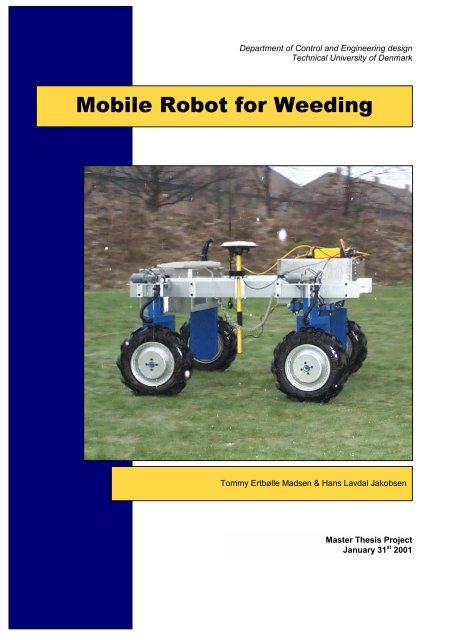
<strong>Mobile</strong> <strong>Robot</strong> <strong>for</strong> <strong>Weeding</strong><br />
Tommy Ertbølle Madsen & Hans Lavdal Jakobsen<br />
Master Thesis Project<br />
January 31 st 2001
Supervisor: Associate professor Ph.d. Torben Sørensen<br />
Tommy Ertbølle Madsen<br />
Student ID: c948429<br />
tommy@ertboelle.dk<br />
Mechanical and control engineering.<br />
Has participated in the development of<br />
the BinderWrap TM round bale wrapper.<br />
www.binderwrap.dk<br />
This project is made by<br />
Hans Lavdal Jakobsen<br />
Student ID: c928543<br />
hans@miditec.com<br />
Electro and control engineering.<br />
Has developed the musicians software<br />
EarMaster TM in his company MidiTec.<br />
www.earmaster.com
Agricultural robot<br />
Abstract<br />
The goal with this master thesis has been to develop an autonomous<br />
agricultural vehicle. The decisions regarding the design of mechanics,<br />
electrics and software are discussed and the experimental results are<br />
presented.<br />
The environmental impact of agricultural production is very much in<br />
focus, while the competition demands high efficiency. Some years<br />
ago, weeding was done manually without the use of pesticides. With<br />
the development of an autonomous agricultural vehicle with sensors<br />
<strong>for</strong> weed detection, it will again be possible to avoid the use of<br />
pesticides.<br />
The vehicle uses high precision GPS (RTK), encoders, compass, and<br />
tilt sensors, to position itself and follow waypoints.<br />
We have developed a module based software system and identified 12<br />
areas of the system (modules) that have each been enclosed in<br />
separate dll's with well defined interfaces. The modules include<br />
interfaces to sensors, low-level and high-level controllers and more.<br />
By using hardware timers, it has been possible to develop a real-time<br />
control system using Windows98.<br />
A vehicle suitable <strong>for</strong> research under field conditions has been<br />
developed. The vehicle has 4-WD and 4-WS, which makes it possible<br />
to test different steering strategies. The vehicle is specially designed<br />
<strong>for</strong> in-row driving; this has been achieved with the use of in-wheel<br />
motors. The vehicle can drive in row crops with a row distance down<br />
to about 250 mm and with 500 mm high crops.<br />
3
4<br />
Synopsis<br />
Agricultural robot<br />
Målet med dette speciale har været at udvikle et autonomt<br />
landbrugskøretøj. Beslutningerne omkring udviklingen af mekanik,<br />
elektronik og software er beskrevet og resultaterne er fremlagt og<br />
diskuteret.<br />
Landbrugsproduktionens miljøbelastning er meget i fokus i dag og<br />
samtidig øges kravene betydeligt til erhvervets konkurrenceevne. For<br />
år tilbage blev ukrudtet i marken fjernet manuelt uden brug af<br />
pesticider. Med udviklingen af et autonomt landbrugskøretøj med<br />
sensorer <strong>for</strong> detektering af ukrudt vil det igen blive muligt at undgå<br />
brugen af pesticider.<br />
Køretøjet er udstyret med højpræcisions GPS (RTK), enkodere,<br />
kompas og tiltsensorer <strong>for</strong> at kunne positionere sig selv og følge en<br />
specificeret rute.<br />
Vi har udviklet et modulbaseret softwaresystem og identificeret 12<br />
dele af systemet (moduler), som hver er placeret i en dll med en<br />
veldefineret grænseflade. Modulerne består af drivere til sensorer,<br />
lavniveau og højniveau regulatorer mm.<br />
Ved at bruge hardware timere har det været muligt at udvikle et<br />
realtidskontrolsystem under operativsystemet Windows98.<br />
Der er udviklet et køretøj specielt til <strong>for</strong>skning under mark vilkår.<br />
Køretøjet har firehjulstræk og styring på alle fire hjul, hvilket gør det<br />
muligt at undersøge <strong>for</strong>skellige styringsstrategier som f.eks. <strong>for</strong>- eller<br />
baghjulsstyring. Konstruktionen er lavet specielt med henblik på at<br />
kunne køre mellem afgrøderækkerne, dette er opnået ved brugen af<br />
navmotorer. Køretøjet kan køre i afgrøder med ned til ca. 250 mm<br />
mellem rækkerne og i ca. 500 mm høje afgrøder.
Agricultural robot<br />
Preface<br />
In this project we have focused on:<br />
- Making a vehicle with optimum design <strong>for</strong> agricultural use: crosscountry,<br />
large ground clearance and slim wheel and transmission<br />
design <strong>for</strong> in-row driving.<br />
- Making a flexible hardware and software design. The vehicle is<br />
designed <strong>for</strong> further experiments and not <strong>for</strong> commercial use. The<br />
design opens up possibility <strong>for</strong> testing sensors, new weeding<br />
technologies and high precision in-row field steering.<br />
- Getting experimental results with RTK/GPS, because we had the<br />
chance to borrow the (so far expensive) equipment. RTK/GPS is a<br />
promising new technology <strong>for</strong> high precision agriculture.<br />
During the development of mechanics, electronics and software we<br />
have focused on making the vehicle flexible. The choice of<br />
technology <strong>for</strong> the various functions has big impact on functionality,<br />
flexibility and per<strong>for</strong>mance.<br />
During the development process we have had safety in the back of our<br />
minds and put an ef<strong>for</strong>t in eliminating or reducing the risks concerning<br />
an autonomous vehicle.<br />
We have been under time pressure all the way; just to get the vehicle<br />
driving. This has <strong>for</strong>ced us to cut corners in some areas, especially the<br />
control engineering area.<br />
Thanks to:<br />
Associate Professor Torben Sørensen <strong>for</strong> your help with robotics and<br />
<strong>for</strong> not setting limits <strong>for</strong> our goal.<br />
Professor Christian Boe <strong>for</strong> your help with design methods and<br />
mechanical reviews.<br />
Associate Professor Nils Andersen <strong>for</strong> letting us draw on your<br />
experiences with autonomous vehicles.<br />
Deputy head of department Svend Christensen, head of research unit<br />
Martin Heide-Jørgensen and senior scientist Henning Tangen Søgaard,<br />
Department of Agricultural Engineering <strong>for</strong> ideas and encouragement.<br />
Ph.d. student Anna B.O. Jensen, National Survey and Cadastre <strong>for</strong><br />
borrowing us the GPS equipment and giving valuable support.<br />
MSc Henrik Holm, Department of Product Development <strong>for</strong> help with<br />
electronics.<br />
Thomas Thriges foundation <strong>for</strong> economical support.<br />
Our wives Karen and Birgitte <strong>for</strong> support and understanding (!)<br />
5
6<br />
Agricultural robot<br />
1. Introduction 8<br />
1.1. PROJECT DESCRIPTION............................................................. 8<br />
1.2. STATE-OF-THE-ART................................................................. 10<br />
1.3. ANALYSES AND PRODUCT SPECIFICATION ........................... 12<br />
2. THE OVERALL PRINCIPAL CONCEPT............................ 15<br />
2.1. TRACTION ............................................................................... 15<br />
2.2. STEERING ................................................................................ 16<br />
2.3. DIMENSIONS............................................................................ 17<br />
2.4. CONTROL ARCHITECTURE .................................................... 19<br />
2.5. MOTORS AND POWER SUPPLY................................................ 25<br />
2.6. SUMMARY OF THE OVERALL CONCEPT CHOSEN .................. 26<br />
3. THE MECHANICAL DESIGN............................................... 27<br />
3.1. STEERING AND DRIVE GEAR................................................... 27<br />
3.2. WHEEL MODULE..................................................................... 31<br />
3.3. CHASSIS................................................................................... 49<br />
3.4. ASSEMBLY............................................................................... 63<br />
3.5. SUMMARY................................................................................ 65<br />
4. COMPUTER AND INTERFACE ........................................... 66<br />
4.1. ELECTRICAL POWER WIRING................................................. 66<br />
4.2. CONTROL CONNECTIONS ....................................................... 67<br />
4.3. HARDWARE HANDLING OF ERRORS....................................... 72<br />
4.4. COMPUTER INTERFACE.......................................................... 76<br />
4.5. COMPUTER POWER SUPPLY ................................................... 78<br />
4.6. COMPUTER MONITOR............................................................. 80<br />
5. SOFTWARE MODULES ........................................................ 82<br />
5.1. SOFTWARE MODULES OVERVIEW.......................................... 82<br />
5.2. MAIN APPLICATION ................................................................ 87<br />
5.3. ENCODERS MODULE ............................................................... 89<br />
5.4. THE GPS MODULE ................................................................. 95<br />
5.5. ORIENTATION MODULE........................................................ 100<br />
5.6. POSITION MODULE................................................................ 110<br />
5.7. VISION MODULE.................................................................... 113<br />
5.8. VISION TASK PLANNER ......................................................... 119<br />
5.9. WAYPOINT MODULE............................................................. 120<br />
5.10. PATH MODULE .................................................................... 121<br />
5.11. CONTROLLER...................................................................... 123<br />
5.12. MOTOR CONTROLLER MODULE......................................... 128<br />
5.13. THE MOTOR OUT MODULE................................................. 134<br />
5.14. TIMER MODULE .................................................................. 137<br />
6. TEST RESULTS ..................................................................... 139<br />
6.1. LOW LEVEL CONTROLLER ................................................... 139<br />
6.2. HIGH LEVEL CONTROLLER .................................................. 143
Agricultural robot<br />
7. RECOMMENDATIONS ....................................................... 151<br />
7.1. HARDWARE........................................................................... 151<br />
7.2. SOFTWARE ............................................................................ 152<br />
7.3. CONTROL ENGINEERING...................................................... 152<br />
8. CONCLUSION ....................................................................... 154<br />
9. LITERATURE........................................................................ 156<br />
9.1. PRIMARY LITERATURE......................................................... 156<br />
9.2. SECONDARY LITERATURE.................................................... 156<br />
9.3. PATENTS................................................................................ 158<br />
9.4. PRODUCT MANUALS ............................................................. 158<br />
9.5. PRODUCT SALES MATERIAL................................................. 158<br />
APPENDIX 1-5 IN SEPARATE VOLUME<br />
CD-ROM WITH VIDEO, CAD MODEL, SOURCE CODE AND OTHER<br />
MATERIAL IN THE BACK OF THIS VOLUME.<br />
7
8<br />
Figure 1.1 Precision farming<br />
1. 1. Introduction<br />
Agricultural robot<br />
1.1. Project description<br />
This project is based on ideas from Svend Christensen, DJF, proposed<br />
at the conference "Technology in the Primary Agriculture" 1999<br />
arranged by the Danish Agricultural and Veterinary Research Council<br />
[HIGHTECH].<br />
Motivation<br />
Today the environmental impact of agricultural production is very<br />
much in focus and the demands to the industry is increasing. The<br />
production of agricultural products is growing and the competition is<br />
getting bigger, there<strong>for</strong>e the farmer has to be very efficient to be able<br />
to compete. At the same time the demands, <strong>for</strong> less use of pesticides<br />
and fertilizers, from the consumer and the legislation are increasing.<br />
There<strong>for</strong>e the farmers have to use high technology in the fields <strong>for</strong><br />
weeding, spraying, etc., earlier weeding were done manually but today<br />
it is neither profitable or possible to get a sufficient number of<br />
labourer <strong>for</strong> this job.<br />
In this project, an autonomous agricultural vehicle, <strong>for</strong> test and<br />
development of sensors, tools and in<strong>for</strong>mation technology in the field,<br />
is going to be developed.<br />
Problem statement<br />
Development and construction of an autonomous robot <strong>for</strong> weed<br />
control in row crops e.g. sugar beets or maize. The robot can be<br />
divided into four main modules:<br />
1. A vehicle as a plat<strong>for</strong>m <strong>for</strong> carrying e.g. weeding tools <strong>for</strong> inrow<br />
weeding. The vehicle could be equipped with the control<br />
modules described below.<br />
2. A control unit, with input from Vision, GPS, and other<br />
necessary sensors, are providing the vehicle and the tools with<br />
the necessary control signals.<br />
3. A GPS module that provides the vehicle with its global<br />
position in real time.<br />
4. A vision system detecting the position of the crop relative to<br />
the vehicle position.<br />
The main goal of this project is the development of the vehicle and the<br />
control unit, with possibility of using different sensor technologies.<br />
We want to test the vehicle and control unit and show that the robot is<br />
capable of following a path under field conditions.<br />
The vehicle<br />
The autonomous vehicle should be developed to test different sensor<br />
systems and tools in the field. The vehicle should be able to work<br />
under field conditions, where the vehicle can be disturbed by<br />
irregularities, when following a specified path.
Agricultural robot<br />
Figure 1.2 Timetable <strong>for</strong> the<br />
project.<br />
The control unit<br />
The control software is intended to be executed on a PC physically<br />
attached to the vehicle. Interface cards, the serial and parallel ports<br />
will be used <strong>for</strong> communication with the peripherals.<br />
The control software is going to be developed with a high level<br />
programming language and is going to work on a Windows operating<br />
system. This is chosen because of our expertise in this area, the<br />
flexibility, and the large number of available interface cards with<br />
drivers.<br />
The control of motors and the higher-level path control are intended to<br />
be solved with classical methods as e.g. PID control.<br />
The GPS module<br />
From the National Surveys and Cadastre, Denmark we were offered<br />
the possibility of borrowing RTK/GPS equipment, which is able of<br />
giving a precision on 1 to 5 cm with a 5 Hz frequency. This sensor<br />
method had earlier been abandoned because of the very high price, but<br />
with the possibility of borrowing the equipment, testing RTK/GPS is<br />
made one of the main goals.<br />
Vision<br />
The development of the vision system is not a primary goal.<br />
There<strong>for</strong>e, we want to make the vision system simple and it should<br />
just be able to recognize spots on the ground with good contrast to the<br />
ground. It should be possible to replace this simple module with more<br />
advanced modules <strong>for</strong> crop recognition in the field.<br />
Related topics<br />
Many interesting topics, like alternative energy sources, power<br />
consumption, data collection, surveillance of the robot from the farm,<br />
etc., can be investigated related to the development of an agricultural<br />
weeding robot. Each of these topics can be subject to years of research<br />
and will there<strong>for</strong>e not be dealt with in detail in this project. The<br />
different problems and tasks, which we will not have the time to<br />
investigate, will be listed in “Recommendations”, page 151.<br />
Project plan<br />
To be able to reach our goal, it is necessary to plan the activities<br />
carefully. The time <strong>for</strong> the project is 3/4 of a year distributed over one<br />
year. The first 6 months are on half time and the last 6 months on full<br />
time. A timetable is made <strong>for</strong> the project, were the start points and<br />
durations of the main activities are listed, see appendix 1.1.1 and<br />
Figure 1.2.<br />
The analysis stage started with brainstorming, literature study and<br />
meetings with people, who have know-how about and interest in the<br />
topic <strong>for</strong> this project. Then the project statement is detailed and a<br />
specification <strong>for</strong> the robot were made and the synthesis is started. The<br />
search <strong>for</strong> principle concepts is made parallel with the vision software.<br />
In August the first CAD drawings are made and the control<br />
architecture is determined. The workshop starts making the parts in<br />
September and the vehicle is ready <strong>for</strong> assembly in late October.<br />
The first tests should have begun primo November. Un<strong>for</strong>tunately, the<br />
assembly and tests of the robot was delayed because we had<br />
9
10<br />
Criteria's<br />
Overall<br />
design<br />
Analysis<br />
Main<br />
functions<br />
Part<br />
functions<br />
and means<br />
Principle<br />
structure<br />
Quantitative<br />
structure<br />
Part design<br />
-Material<br />
-Dimensions<br />
-Finish<br />
Figure 1.3 Product synthesis<br />
model [TJALVE]<br />
Figure 1.4 Advanced Tool Control<br />
from Eco-Dan (between the tractor<br />
and the cultivator)<br />
Agricultural robot<br />
underestimated the time necessary in the workshop. There<strong>for</strong>e, more<br />
of the documentation has been made parallel with the development of<br />
the robot and the first outdoor tests did not begin until primo January.<br />
Because the test started so late, we have not had time <strong>for</strong> optimising<br />
the controllers, which we had chosen.<br />
Means (Tools and resources)<br />
Tools<br />
In the project we have mainly used methods <strong>for</strong> systematically design<br />
of industrial products (Figure 1.3) and classical control methods<br />
lectured at IKS.<br />
Most of the design has been done with help from different computer<br />
tools. The software is developed in Delphi and the mechanical design<br />
is detailed with Pro-Engineer. For calculations Matlab, Excel and<br />
Win-Beam have been used.<br />
Resources<br />
From the start, we had identified different departments and people,<br />
who could help us with know how. The Department of Control and<br />
Engineering Design (IKS), the IKS-workshop, the Department of<br />
Agricultural Engineering (DJF), Department of Automation (IAU),<br />
the Department <strong>for</strong> Product Development (IPU), National Cadastre<br />
and Survey (KMS), see appendix 1.1.2.<br />
The budget <strong>for</strong> master projects is very limited, but because this project<br />
can be used <strong>for</strong> further research, it has been possible to get the<br />
necessary economical resources. The robot is the property of IKS,<br />
who has paid most of the robot, in addition Thomas B. Thriges<br />
Foundation has given 22.000,- kr to the project (Appendix 1.2.2-3).<br />
1.2. State-of-the-art<br />
This paragraph will describe the current technological level <strong>for</strong><br />
precision farming in row crops. The content is based on a literature<br />
study (appendix 1.2.1.d and literature list), internet study and<br />
in<strong>for</strong>mation from DJF.<br />
State-of-the-art commercial products<br />
So far autonomous in-row vehicles <strong>for</strong> weed control have not been<br />
commercialised, but control systems <strong>for</strong> controlling the implements<br />
towed by the tractor are available. Some products can also control the<br />
tractor in the row, but it still needs to be monitored carefully by the<br />
driver. The technology used in these commercial products is computer<br />
vision and ultrasonic sensors.<br />
Vision and ultrasonic sensors<br />
The first company to launch vision control is Eco-Dan A/S, who has<br />
developed a system called Advanced Tool Control (ATC), see Figure<br />
1.4. The system consists of two dedicated vision cameras and a<br />
dedicated microprocessor <strong>for</strong> manipulating the pictures and generating<br />
the control signal <strong>for</strong> positioning the implement sideways. The system<br />
makes it possible <strong>for</strong> one man to manoeuvre a cultivator with a<br />
precision of +/- 3 cm with speeds up to 8 – 10 km/h in the field.
Agricultural robot<br />
Figure 1.5 John Deere Pilot<br />
System<br />
Figure 1.6 The Fieldstar<br />
precision farming concept.<br />
John Deere and Danfoss/Reichardt have developed a system using<br />
ultrasonic sensors. We do not know the precision of this system, but it<br />
is mainly <strong>for</strong> relieving the driver when following swaths and not <strong>for</strong><br />
high precision control in row crops, see Figure 1.5.<br />
DGPS in precision farming<br />
The last few years DGPS with a precision of 1 – 2 m has become quite<br />
popular <strong>for</strong> yield monitoring. The concept is that the combine<br />
equipped with DGPS makes a yield map and this in<strong>for</strong>mation together<br />
with soil analyses from the field helps the farmer to differentiate the<br />
amount of fertilizer used in the field. In this way the farmer can<br />
optimise the use of fertilizer. He also gets a better overview of his<br />
production, which can help him to make the right decisions about the<br />
use of his fields.<br />
RTK/GPS<br />
So far, high precision GPS like RTK has not been used commercially<br />
in the agricultural industry <strong>for</strong> controlling the position of vehicles or<br />
implements.<br />
The development of a RTK/GPS reference system in Denmark is<br />
going very fast at the moment. Already now it is possible to subscribe<br />
to a service delivering the reference signals via the GSM net, then it is<br />
not necessary to set up a local base station (www.gpsnet.dk). This is a<br />
large step towards commercial agricultural use of high precision GPS.<br />
Crop sensors<br />
Hydro has developed a sensor to detect the amount of nitrogen in the<br />
crop. The sensor is an optical sensor that can measure the amount of<br />
chlorophyll in the crop, which gives a good estimate of the nitrogen<br />
level. The sensor is mounted on the roof of the tractor and connected<br />
to a computer, which controls the amount of fertilizer to be spread.<br />
Research results<br />
This paragraph only describes the most relevant research result we<br />
have found in relation to our project. An exhaustive list of the<br />
literature studied can be found in the literature list.<br />
Vision<br />
Test results from Cali<strong>for</strong>nia research on spot spraying and<br />
identification of weeds and crops are not very convincing. 24.2% of<br />
the tomatoes were sprayed and 52.4% of the weeds were not sprayed<br />
[TOMATO]. It is very difficult to identify the different species and it<br />
will take years of research to make a satisfactory identification.<br />
DGPS<br />
At Stan<strong>for</strong>d University an automatic tractor guidance system using<br />
carrier-phase differential GPS has been developed [GPSTRAC]. They<br />
use four GPS antennas on the roof of a tractor to measure both the<br />
position and attitude of the tractor. Very good results have been<br />
achieved in the field following non-linear trajectories with a controller<br />
using a priori in<strong>for</strong>mation about the trajectory.<br />
11
12<br />
Figure 1.7 Identify the life stages<br />
of a product.<br />
Figure 1.8 Cornfield sown with<br />
double distance (250 mm) between<br />
the rows <strong>for</strong> mechanical weeding.<br />
Agricultural robot<br />
At the Institute of Agricultural and Environmental Engineering,<br />
IMAG-DLO, the Netherlands researchers have experimented with<br />
controlling the lateral movement of the implement using RTK/DGPS.<br />
The tests showed an average error of 1 cm at an average speed of 3.6<br />
km/h [GPSIMP].<br />
Off-road and agricultural vehicles<br />
Analogies and comparable products can often provide useful<br />
in<strong>for</strong>mation and give ideas <strong>for</strong> generating concepts. There<strong>for</strong>e, other<br />
off-road and agricultural vehicles have been examined to see if this<br />
could give some help. In appendix 1.2.1.a-c some of the examined<br />
products can be seen.<br />
1.3. Analyses and Product<br />
Specification<br />
In this paragraph the different life stages of the product are identified<br />
and analysed and the demands, criteria’s and comments are<br />
summarized in a product specification, appendix 1.3.5.a-b.<br />
In the product specification solutions are delimited from not solutions<br />
(demands) and a yardstick <strong>for</strong> the solution is specified (criteria’s). It is<br />
important to go through all life stages and remember all the<br />
stakeholders to specify the product right. The product specification is<br />
a management tool <strong>for</strong> controlling, that the right product is designed.<br />
On the other hand, the product specification should only set the<br />
relevant and necessary constraints <strong>for</strong> the product. The specification is<br />
not a static paper, but can be altered during the design process in<br />
dialogue with the relevant persons.<br />
As the solution is designed in detail, it can be necessary to add<br />
additional demands and criteria’s to the specification or make a sub<br />
specification. If e.g. a modular design is chosen, it can be necessary to<br />
make individual specifications <strong>for</strong> each module, because the other<br />
modules sets additional demands and criteria’s to the design.<br />
Identification of life stages<br />
This product is only <strong>for</strong> research purposes and is there<strong>for</strong>e not going<br />
through all the life stages of a "normal" product. The life stages of this<br />
product are: design, industrial design, production, service, use,<br />
transport, destruction. Use is divided into: input, output, users,<br />
environment and safety.<br />
Background material <strong>for</strong> the Product Specification<br />
The product specification is based on input from literature, DJF and<br />
our own knowledge about agriculture and particularly field conditions.<br />
Some of the demands and criteria's have been determined from the<br />
beginning (appendix 1.3.1-1.3.4) others have been identified but have<br />
not been answered until later in the project.<br />
The paragraphs below are comments referring to the product<br />
specification in appendix 1.3.5.a-b.<br />
Design<br />
The 3/4-year available <strong>for</strong> this project is the main constrain on the<br />
design stage.
Agricultural robot<br />
Figure 1.9 Very low turning<br />
radius.<br />
Figure 1.10 The ideal soil<br />
structure.<br />
Industrial design<br />
This is not a commercial product, which should appeal to a customer.<br />
However, future students could also be seen as customers and it is<br />
important that the robot will make students enthusiastic and wanting<br />
to work in this area. There<strong>for</strong>e, the robot should appear as a<br />
functional, high tech and innovative product.<br />
Production<br />
This robot is a prototype <strong>for</strong> research and the budget is limited,<br />
there<strong>for</strong>e many processes and materials are not economical to use. The<br />
robot should be built at the IKS workshop, which is specialized in<br />
making prototypes and small batch production. The main<br />
qualifications are:<br />
• High precision metalwork<br />
• Mass reducing processes (several high precision CNC<br />
machines)<br />
• Welding<br />
• Press brake bending in sheet metal<br />
Service<br />
The robot should be easy to service and parts should be easy to<br />
replace. Students, researchers and technical staff at the institute will<br />
carry out the work.<br />
Use<br />
The robot is <strong>for</strong> research in methods <strong>for</strong> sustainable weed control and<br />
control engineering.<br />
The vehicle should be able to operate at a speed about 0.5 – 1 m/s and<br />
drive <strong>for</strong> about 2 – 4 hours between recharging.<br />
The precision of the vehicle must be within ±5 cm to drive without<br />
damaging crops in cornfields. In crops with bigger row distance the<br />
demand is not so high. But if the vehicle is driving precisely, then it<br />
will be easier to control the tool or maybe it will not even be necessary<br />
to control the tool relative to the vehicle.<br />
The dimensions of the vehicle should make it capable of driving in<br />
row crops with 500 mm between the rows. The clearance between the<br />
vehicle chassis and the ground should be 500 mm to allow corn to<br />
pass below the vehicle.<br />
The vehicle should be able to turn with a small turning radius on the<br />
headlands. It is not a demand that it should be able to turn as sharply<br />
as on Figure 1.9.<br />
-Input<br />
The vehicle should be able to use RTK/GPS position <strong>for</strong> steering in<br />
rows in e.g. cornfields or beet fields. It is also wanted to test the<br />
vehicle using vision.<br />
-Output<br />
The vehicle should be capable of carrying different tools <strong>for</strong> weed<br />
removal or data collection in the fields.<br />
-Users<br />
The users are primarily students and researchers with expert<br />
knowledge. It should be easy to access the different components and<br />
test different tools and sensors. The software should be modular, so<br />
that test of different controllers and sensors does not require changing<br />
all the software.<br />
13
14<br />
Figure 1.11 The vehicle will be<br />
exposed to different weather<br />
conditions.<br />
Agricultural robot<br />
-Environment<br />
The vehicle should be able to operate in fields after sowing. The<br />
machine is made <strong>for</strong> Danish conditions and <strong>for</strong> test purposes, there<strong>for</strong>e<br />
the fields are assumed nearly level with maximum gradients on about<br />
10%. The ideal field is shown on Figure 1.10, but the conditions can<br />
vary a lot.<br />
The vehicle should be able to operate both in rainy and sunny weather.<br />
It is there<strong>for</strong>e important to enclose parts, which can be damaged by<br />
water and dust.<br />
-Safety<br />
It is very important, that the vehicle is safe to work with, so that<br />
people are not injured. Secondary it is important that the vehicle is not<br />
damaged or is causing damage to the surroundings.<br />
There is no special rules concerning the use of mobile robots and since<br />
this robot is not <strong>for</strong> commercial use the general rules do not have to be<br />
meet [DEMKO]. We do however want to look at the general safety<br />
problems of autonomous vehicles and to make the developed vehicle<br />
as safe as possible.<br />
Transport<br />
It should be possible to transport the robot on a car trailer or in a van.<br />
Destruction<br />
Electronics should be removed disposed separately, but the disposal<br />
does not give rise to any special demands to the vehicle design.
Agricultural robot<br />
Figure 2.1 Ground pressure of<br />
tracked vehicle<br />
Figure 2.2 Ground pressure of<br />
wheeled vehicle.<br />
Figure 2.3 Climbing capability of<br />
vehicles with FWD, RWD and All-<br />
WD.<br />
A<br />
Figure 2.4 A towed wheel passing<br />
an obstacle.<br />
2. The overall principal<br />
concept<br />
This chapter will document the considerations made about the<br />
principles of the vehicle and the choice of concept <strong>for</strong> the mobile<br />
robot. The principles considered is: traction, steering, dimensions,<br />
power supply and control architecture.<br />
2.1. Traction<br />
The traction methods have big influence on the steering and terrain<br />
properties, cost and power consumption of the vehicle.<br />
Wheels, tracks, feet or air cushion<br />
Feet would not be feasible <strong>for</strong> this robot; hence, the technology is not<br />
mature.<br />
An air cushion will damage the crop and raise a lot of dust, which will<br />
cover the crop and set very high demands to the dust tightness of the<br />
vehicle.<br />
Tracked tractors are quite common on big farms with big fields and<br />
little need <strong>for</strong> road transportation, because of low ground pressure and<br />
very good drawbar pull per<strong>for</strong>mance on soft and loose soil. These<br />
properties are not so important <strong>for</strong> the mobile robot, where important<br />
properties are steering precision, low power consumption and low<br />
cost. To develop tracks <strong>for</strong> the robot would also be too big a task <strong>for</strong><br />
this project.<br />
Wheels are inexpensive and because of the little need <strong>for</strong> drawbar pull<br />
and load carrying capacity the bigger sinkage and ground pressure is<br />
of little importance. The soil conditions in fields after sowing are also<br />
normally good <strong>for</strong> wheeled vehicles and there<strong>for</strong>e wheels are chosen<br />
<strong>for</strong> traction (appendix 2.1.1).<br />
FWD, RWD or All-WD<br />
The choice of which wheels should be driving depends on the steering<br />
strategy, which will be discussed in following passage. In this<br />
passage, some general things about front, rear and all wheel drive will<br />
be addressed.<br />
The diagram on Figure 2.3 shows the possible climbing versus the<br />
friction coefficients and it can be seen that 4-WD gives the best grip.<br />
This is because the whole weight of the vehicle creates traction<br />
between wheels and road. The second best is rear 2-WD, because a<br />
part of the weight on the front wheels is on the rear wheels, when<br />
driving up hill. [AB86]<br />
On Figure 2.4 a towed wheel is shown being towed over an obstacle.<br />
The momentum equation around the point A shows that it is necessary<br />
with a big <strong>for</strong>ce Ft to lift the normal <strong>for</strong>ce on the wheel Fg. As it can be<br />
seen the <strong>for</strong>ce will be infinite, when the height of the obstacle is as<br />
high as the wheel radius. The maximum <strong>for</strong>ce <strong>for</strong> a driving wheel is<br />
equal to the <strong>for</strong>ce Fg, when the obstacle is higher than the wheel<br />
radius. However, if the obstacle is so high, the wheel will have no grip<br />
unless it is pushed against the obstacle. To get the best terrain<br />
15
16<br />
Figure 2.5 Skid steer loader.<br />
Figure 2.6 Principle of All-WD<br />
differential steering.<br />
Figure 2.7 <strong>Robot</strong> with 2WD<br />
differential steering.<br />
Figure 2.8 Principle of 2WD<br />
differential steering.<br />
Agricultural robot<br />
per<strong>for</strong>mance it is necessary with 4-WD, were all wheels helps the<br />
vehicle to overcome obstacles. (Appendix 2.1.3.c and 2.3.3.a)<br />
2.2. Steering<br />
It is important <strong>for</strong> the vehicle to be able to steer very precisely in the<br />
crop rows and also to make as little damage as possible to the crop. In<br />
the following advantages and disadvantages of different steering<br />
strategies will be discussed.<br />
Differential steering<br />
The principle of differential steering is to make a difference between<br />
the speeds of the wheels on the left hand side compared to the speeds<br />
of the wheels on the right hand side. The difference in speed will<br />
make the vehicle turn. It makes a big difference to use this method on<br />
an all-wd vehicle compared to a 2WD vehicle, which will be<br />
discussed in the following paragraph.<br />
All-wd<br />
Differential steering is often used <strong>for</strong> vehicles that should be very<br />
maneuverable in difficult terrain. A vehicle using this steering method<br />
can turn on the spot and the method is often seen on earth moving<br />
equipment like skid steer loaders Figure 2.5. The transmission is also<br />
simple to construct, because the wheels in one side is turning at the<br />
same speed and the position and orientation of the wheels are fixed.<br />
This indicates that it could be a possible solution <strong>for</strong> a weeding robot,<br />
but the method also has some major disadvantages. In a turn the<br />
vehicle also turns around a vertical axis through the center of the<br />
vehicle, which means that the wheels have to slide sideways. This<br />
uses a lot of power to turn the vehicle. The method is also unsuitable<br />
<strong>for</strong> dead reckoning because of the excessive slip, which makes<br />
odometer data useless. Damage to the crop is also likely to happen.<br />
The wheels will dig out viable weed seeds, which will germinate.<br />
Because of these disadvantages we have chosen not to use differential<br />
steering all-wd (skid steering). (Appendix 2.1.2.a-d)<br />
2-wd<br />
When using 2WD differential steering one or more castor wheels<br />
support the vehicle. A vehicle using this steering method can turn on<br />
the spot. The method is often used in robotics <strong>for</strong> e.g. AGV´s because<br />
of the very good maneuverability. But because of the castor wheels it<br />
is not suitable <strong>for</strong> off-road driving.<br />
When the vehicle is turning, it has to drag the castor wheels. Even a<br />
small obstacle will demand a big <strong>for</strong>ce from the driving wheels,<br />
because of the momentum arm from the turning center to the castor<br />
wheel.<br />
We have made some tests with a small trolley with castor wheels on a<br />
lawn and on paved ground, see appendix 2.1.3.d. The tests showed<br />
that it is necessary with a <strong>for</strong>ce 2 – 3 times bigger than the normal<br />
<strong>for</strong>ce from the driving wheels, to drag the castor wheels in a turn.<br />
This steering method is not chosen because of its poor off-road<br />
characteristics. (Appendix 2.1.3.a-d)
Agricultural robot<br />
Figure 2.9 Tractor with articulated<br />
steering and the steering principle.<br />
Figure 2.10 Principle of Ackerman<br />
steering.<br />
Figure 2.11 Placement of wheels<br />
on the robot.<br />
Articulated steering<br />
The principle of articulated steering is to change the angle between the<br />
front axle and the rear axle of a vehicle. The disadvantage of this<br />
method is that there is little space <strong>for</strong> tools between the front and rear<br />
axle. Poor stability in turns can also be a problem, because of the<br />
transversal movement of the center of gravity. An advantage is the<br />
simplicity of the construction and good capability of following rows,<br />
see appendix 2.1.4.<br />
Changing heading of wheel(s)<br />
This is the principle that most road vehicles use <strong>for</strong> steering. When the<br />
<strong>for</strong>ces on a vehicle are ignored, Ackerman describes the ideal relation<br />
between the angles of the outside and inside wheel in a turn. If the<br />
relation between the wheel angles follows the Ackerman equation,<br />
geometrically induced tire slippage will be eliminated. (Centripetal<br />
<strong>for</strong>ces are ignored and there<strong>for</strong>e this only apply <strong>for</strong> very low turning<br />
speeds in practice) The low geometrically induced tire slippage is<br />
important to get good odometer data and steer precisely.<br />
The Ackerman criterion is very difficult to implement mechanically,<br />
because it is highly non linear. There<strong>for</strong>e on most vehicles the steering<br />
angles only approximate the Ackerman criterion <strong>for</strong> small steering<br />
angles. However, deviations from Ackerman do not necessarily mean,<br />
that the steering geometry is not optimal under real driving conditions<br />
at higher speeds.<br />
If the vehicle is not all-wd, it has the same problems as the model with<br />
castor wheels. It is necessary with big <strong>for</strong>ces to turn, when a towed<br />
wheel hits an obstacle. If the wheels, which are used <strong>for</strong> steering, are<br />
towed, they can have problems with getting a grip in loose soil <strong>for</strong><br />
turning the vehicle. This will give wheel slippage a low steering<br />
precision.<br />
If the vehicle has all-wd it will have very good off-road properties.<br />
The vehicle can steer on just one axle or all axles. If the weeding robot<br />
can steer on all axles it will be possible to obtain a very small turning<br />
radius. The wheels will in a stationary turn follow the same tracks if<br />
the steering of the rear and front wheels are symmetric about the<br />
middle of the vehicle (Figure 2.11). There<strong>for</strong>e, the vehicle needs very<br />
little space between the rows to follow the rows precisely.<br />
The disadvantage of steering on all wheels is that the construction and<br />
control become more complex.<br />
Because of the possibility of good odometer data, precise steering and<br />
small turning radius, all-wheel Ackerman steering have been chosen.<br />
2.3. Dimensions<br />
Four wheels placed in each corner of a rectangle with the length<br />
parallel to the crop rows have been chosen <strong>for</strong> the vehicle. This<br />
configuration gives a good stability and the rear wheels can run in the<br />
tracks of the front wheels, which decreases the rolling resistance. The<br />
configuration can be seen on Figure 2.11.<br />
Other possible wheel configurations are shown in appendix 2.3.1.d.<br />
The symmetric placement of the wheels and the choice of 4WS and<br />
4WD, give the possibility of making transmission and steering gear in<br />
four identical modules. This will make the mechanical design faster<br />
and especially the construction in the workshop will be faster and less<br />
expensive because of fewer different parts. Planning, interpretation of<br />
17
18<br />
Figure 2.12 Necessary wheel<br />
gauge <strong>for</strong> in-row driving in corn<br />
and beet fields.<br />
Figure 2.13 Possible areas <strong>for</strong><br />
attaching tools<br />
Figure 2.14 Spot sprayer<br />
Figure 2.15 Rotating hoe<br />
Agricultural robot<br />
drawings and adjustment of machines is time consuming in the<br />
workshop and there<strong>for</strong>e it is important to keep the number of different<br />
parts low. This modular concept will then consist of a chassis with 4<br />
identical "wheel modules".<br />
Gauge<br />
There are several constraints on the dimensions of the vehicle. It<br />
should be able to drive in crop rows, with 500 mm between the rows<br />
e.g. sugar beet. There is also focus on weeding in cornfields. <strong>Weeding</strong><br />
is possible when the row distance is increased to 250 mm There<strong>for</strong>e it<br />
would be advantageous that the vehicle could drive in cornrows, with<br />
250 mm between the rows. Beets are broad-leaved and there<strong>for</strong>e the<br />
wheels should not get too close to the row centre and damage the<br />
beets.<br />
This means that the gauge should be either 500 mm or 1000 mm. If<br />
the gauge is 750 mm or 1250 mm the wheels will get to close to the<br />
row centre in beets, a even bigger gauge will make the vehicle too<br />
difficult to transport and handle in general. The ground clearance on<br />
500 mm makes it necessary to make the gauge 1000 mm, because the<br />
centre of gravity else will be placed very high compared to the gauge<br />
and make the vehicle unstable.<br />
Another possibility is to make the gauge adjustable, but we have<br />
judged, that a fixed gauge on 1000 mm. will cover the necessary row<br />
widths sufficiently.<br />
Placement of tools and loads<br />
The tools should be placed in the most stable position with the bestdefined<br />
distance to the ground. The best position is in the middle of<br />
the wheelbase, where obstacles and irregularities will cause minimum<br />
movement of the tool.<br />
Tools<br />
This test vehicle should be able to be tested, with a big variety of tools<br />
<strong>for</strong> weeding, spraying, collection of crop data and soil samples, etc.<br />
This type of vehicle is not intended <strong>for</strong> cultivating etc., which is much<br />
more efficient with conventional tractors. There<strong>for</strong>e this vehicle is not<br />
designed <strong>for</strong> big drawbar pull, but just to be able to transport itself,<br />
tool and a load of e.g. herbicides, under the conditions given in the<br />
field.<br />
DJF has proposed some tool concepts, which the vehicle should be<br />
able to operate with.<br />
Spot sprayer<br />
The idea is to identify the individual weeds and spray the weed leaves,<br />
without polluting the bare ground or the crop. This principle has also<br />
been used <strong>for</strong> spraying railway tracks <strong>for</strong> weeds, which is a simpler<br />
task, because all vegetation must be sprayed.<br />
Rotating hoe<br />
As shown on Figure 2.15 this tool consist of a rotating hoe, which is<br />
synchronized with the <strong>for</strong>ward speed and the position of the crop.<br />
The tool will be able to remove weed between the crops without the<br />
use of herbicides. The disadvantage is the power consumption of the<br />
tool and possible influence on the steering of the vehicle.
Agricultural robot<br />
Figure 2.16 Dimensions<br />
Wheelbase<br />
A short wheelbase improves the manoeuvrability of the vehicle, but<br />
also makes it harder to control. Our goal is to make the vehicle<br />
flexible, there<strong>for</strong>e the wheelbase is chosen so, that it will just leave<br />
room <strong>for</strong> the tools and give the best manoeuvrability.<br />
The rotating hoe and the space <strong>for</strong> rotation of the wheels limit the<br />
wheelbase to minimum 1000 mm, see Figure 2.16. This wheelbase<br />
also allow <strong>for</strong> leave raisers on the wheels to prevent damage to the<br />
crop.<br />
Ensuring ground contact<br />
The wheels should always have contact to the ground to improve<br />
traction and steering and to make the tools follow the ground in a<br />
better defined way. On road vehicles, different spring-damper systems<br />
are used <strong>for</strong> this purpose. On this low speed off-road vehicle, it is not<br />
necessary with more damping than the tyres can provide. However, to<br />
make the wheels follow the ground there has to be a longitudinal pivot<br />
joint between the front and the rear axle. On Figure 2.16 the front axle<br />
can turn about a longitudinal axis, because of the rotational joint in the<br />
middle of the front axle.<br />
2.4. Control Architecture<br />
Sensors<br />
GPS system<br />
During our initial investigations, we found that an af<strong>for</strong>dable GPS<br />
system was not precise enough (the precision of DGPS is 1-5m). To<br />
get a satisfactory precision of 1-5 cm it would require a carrier-phase<br />
differential GPS (also called RTK) equipment priced at about DKK<br />
300.000.<br />
There<strong>for</strong>e we decided not to use GPS, but later we got the possibility<br />
to borrow such equipment from the National Survey and Cadastre<br />
Denmark. Read more in “The GPS Module”, page 95.<br />
Orientation<br />
It is very important to know the orientation of the vehicle, not only the<br />
heading but also the tilt in both directions. For example, the GPS only<br />
returns the position of the GPS antenna. We need to know the roll,<br />
pitch, and compass angles to convert the antenna position to the<br />
control point. The compass angle (yaw) is also important to steer the<br />
vehicle.<br />
To find the orientation of the vehicle different sensors can be used.<br />
We have considered various technologies with various technical pros<br />
and cons, but as our budget is limited, the price is also an important<br />
factor:<br />
Gyroscope.<br />
A gyro can measure the orientation of all three axes. A gyro is<br />
sensitive to the rotation of earth (unless they have build-in<br />
compensation) and they all have to be initialized in a known<br />
orientation. The advantage is that it is not sensitive to accelerations.<br />
19
20<br />
Agricultural robot<br />
The cheapest solution we could found was the electronic dual-axis<br />
“Micro gyro 100” from www.gyration.com which in the spring 2000<br />
was priced US$450.<br />
Accelerometers<br />
There are various technologies to measure acceleration. By measuring<br />
the angular rate on three axes, it can find the orientation relative to the<br />
orientation when it was initialised. This is similar to a gyro and some<br />
manufacturers market accelerometers as electronic gyros.<br />
GPS<br />
With a GPS antenna we get the position in three dimensions. Having<br />
three GPS antennas it is possible to calculate the orientation of all<br />
three axes. It requires several meters between the antennas and high<br />
precision GPS such as carrier-phase differential GPS with a precision<br />
of 1-5 cm. The price <strong>for</strong> this solution is extremely high. Results with 4<br />
antennas on an autonomous guided tractor can be found in<br />
[GPSTRAC].<br />
Magnetometer<br />
The field of the earth can be measured with a 3-axis magnetometer.<br />
The measurement is influenced by the magnetic declination and<br />
deviation caused by local magnetic fields. (Read more about these<br />
errors on page 100). We were recommended to use products from the<br />
companies Billingsley and Bartington by people connected to the<br />
“Ørsted” project. Their products were however quite expensive and<br />
we found other solutions <strong>for</strong> example the Vector 2x from<br />
www.precisionnav.com at only US$ 50.<br />
To calculate the heading from a magnetic field it is required to have<br />
data from an inclinometer (tilt-sensor).<br />
Inclinometer<br />
An inclinometer measures the angle of gravity on two axes. We found<br />
an optical inclinometer from www.usdigital.com priced at US$ 75. It<br />
is based on a damped pendulum with a quadrature encoder and<br />
measures an absolute angle of gravity.<br />
Solution<br />
From Precision Navigation (www.precisionnav.com) we also found<br />
another module than the one mentioned above. It is an all-in-one<br />
product that perfectly suits our needs. It was priced at a reasonable<br />
$345 that with academic discount became $245. It contains a 3-axis<br />
magnetometer and a fluid based tilt-sensor. It compensates <strong>for</strong> tilt<br />
internally, and via the RS232 interface we can read compass and 2<br />
axis tilt data. Read more in the “Orientation module”, page 100.<br />
Vision<br />
So far the most successful way to find plants it is to use a camera.<br />
Usually it would look at the infrared spectrum in which plants show<br />
up clearly from the background. There are already systems in use that<br />
can detect plants but the technology to separate weed from crop is not<br />
yet convincing.<br />
At the “Department of Control and Engineering Design” they already<br />
had a cmos camera used in previous vision projects so there was not<br />
very much <strong>for</strong> us to decide. It does however not look at the infrared
Agricultural robot<br />
spectrum and there<strong>for</strong>e it can only detect “paper plants” with good<br />
contrast to the background.<br />
However, a cmos camera is the best technology <strong>for</strong> use in control<br />
applications. Read more in the “Vision module” on page 113.<br />
Motor feedback<br />
We need to get speed and position feedback from the motors to<br />
control them.<br />
Tachometer<br />
A tachometer returns the current speed and is there<strong>for</strong>e useful <strong>for</strong><br />
speed control. To get the position of the motor we need to integrate<br />
the tachometer output. As the speed output is an analogue signal, it is<br />
sensitive to noise. The noise will also be integrated and the result is a<br />
position error. The integration will typically be done with a computer<br />
sampling the analogue signal through an AD converter. The sample<br />
and hold and quantification of the signal will also introduce a position<br />
error.<br />
Encoders<br />
An alternative is encoders, which read the current position of the<br />
motor. An absolute encoder always knows its position i.e. it does not<br />
have to be initialised. An incremental encoder sends pulses to a<br />
counter and thus the position is always relative. This can be solved by<br />
using an index marking that resets the counter at a certain position. An<br />
encoder is excellent to get the position, but deriving speed from<br />
counter values introduce a quantification error. Especially at low<br />
speed and at high sample rates there might only be a few counter<br />
values between two samples to derive the speed from.<br />
For the steering motors, we need to know the absolute position. An<br />
absolute encoder from www.usdigital.com is US$ 270 while an<br />
incremental encoder with index from the same company is US$ 48.<br />
However when including the cost to interface four of them with the<br />
PC it is US$275 <strong>for</strong> the absolute encoder and US$136 <strong>for</strong> the<br />
incremental encoder.<br />
For the drive motors a tachometer could be used, as we are mainly<br />
interested in controlling speed and not the position. For the dead<br />
reckoning system, we do however need to know the travelled distance<br />
and with the integration errors described above we have chosen<br />
incremental encoders. From www.usdigital.com we found an<br />
incremental encoder that could produce 8192 counts per revolution<br />
which is enough to get a good precision when deriving speed. Read<br />
more about this in the “Encoders module” on page 89.<br />
Hardware<br />
Distributed control<br />
For data communication in commercial or industrial applications, the<br />
CAN-Bus is often used when having a large number of sensors<br />
supplying data <strong>for</strong> a large number of units. The CAN-bus is a<br />
distributed network system. All units connected to the bus have access<br />
to all data on the bus. A sensor will send data on the bus with a<br />
priority and a unique ID. All other receivers can then decide if they<br />
21
22<br />
Agricultural robot<br />
will use this data or not. The advantage is that the cabling is simple as<br />
only one set of cables will connect all units. The disadvantage is that<br />
you need a microcontroller <strong>for</strong> all units interfacing to the bus. This<br />
makes it expensive unless you buy a large quantity.<br />
Centralized control<br />
A cheap and flexible solution is to wire all control signals to interface<br />
cards in a PC. All connections between sensors and the users of sensor<br />
data are made by the PC and all calculations are made in the software.<br />
In this way it is very easy to make modifications as they only have to<br />
be changed in one place. The PC also gives great possibilities to make<br />
an in<strong>for</strong>mative interface to the user.<br />
We have chosen to use a PC as this vehicle is going to be used as a<br />
base <strong>for</strong> many future projects.<br />
Navigation<br />
Manual control<br />
The vehicle should be easy to manoeuvre manually. A cheap, simple<br />
and well-known solution is to use a PC game joystick. The keyboard<br />
could also be used, but as the keys only offer on/off position it is<br />
difficult to control the speed and turning rate precisely. We have<br />
there<strong>for</strong>e chosen to use a joystick. In addition a modern PC joystick<br />
often offers extra sliders and buttons that can be used by the user to<br />
control and activate special functions such as turning sensitivity,<br />
sideways driving, etc.<br />
Automatic control<br />
Position<br />
We borrow the GPS equipment and there<strong>for</strong>e the vehicle must be able<br />
to drive without that. A typical way of getting the position when no<br />
absolute position sensor is available is to use encoder and compass<br />
data in a dead reckoning system. The dead reckoning continuously<br />
calculates the position of the vehicle by summating wheel distances<br />
and vehicle headings. With a well designed dead reckoning system we<br />
are able to use and test the vehicle no matter if the GPS is present or<br />
not. The only difference will be the actual precision of the position.<br />
Path<br />
The robot should be able to follow a list of waypoints. It could <strong>for</strong><br />
example be a list of crop positions generated when sowing. The<br />
waypoints could however also be generated by the on-board vision<br />
system the calculates the position of the plants it sees on the fly.<br />
The vehicle should not necessary drive the direct way between two<br />
waypoints. Especially it might not be possible <strong>for</strong> it to turn sharp<br />
enough to go directly to the next waypoint. This could happen at the<br />
end of a crop row where it should turn 180° and go back with the next<br />
row.<br />
Position control<br />
There are many methods to let a vehicle follow a path. We have<br />
chosen to use a simple solution to start with. The method is often used<br />
when an AGV should follow a line on the ground using optical<br />
sensors.
Agricultural robot<br />
Motor control<br />
We need to control the absolute position of the steering motors. As the<br />
friction to the ground vary a lot there must be an integrator in the<br />
controller to be sure that it can reach the wanted position. We have<br />
decided to use PI controllers<br />
For the Honda drive motors we need a speed control and as the rolling<br />
resistance (including climbing hills) varies a lot there must be an<br />
integrator to use its power potential.<br />
Software<br />
The software should be as flexible as possible and it should be easy<br />
<strong>for</strong> other projects to continue our work without having to start from<br />
the beginning. Software code made by others is especially difficult to<br />
understand and to develop further, because all people have their own<br />
programming style and preferred programming language. Especially<br />
when considering the risk of hidden errors in the code, few people<br />
would there<strong>for</strong>e wish to develop new code directly in the code from<br />
previous projects.<br />
To avoid this problem we decided to make a module based software<br />
system. All the software functionality should be divided into a number<br />
of logical modules that are each compiled into separate DLL’s. The<br />
DLL’s should have a standardized interface just like all Windows<br />
drivers. Each DLL can there<strong>for</strong>e be replaced by another DLL with the<br />
same interface, without affecting the functionality of the rest of the<br />
system. A replacement DLL can even be programmed in any<br />
programming language.<br />
It is there<strong>for</strong>e easy to modify and develop the system without needing<br />
to consider and understand completely what is going on in the other<br />
modules.<br />
Identifying modules<br />
In the first phases of the development we had divided the software<br />
system into 5 modules. The overview of the structure is shown in<br />
appendix 5.0b modules. We soon realized that this was not enough<br />
and we there<strong>for</strong>e added 7 more modules.<br />
In the following sections we will argue <strong>for</strong> the choice of the final set<br />
of modules.<br />
Hardware<br />
It should be possible to replace the attached hardware (sensors and<br />
DA converters) without affecting the other parts of the system.<br />
There<strong>for</strong>e there should be a module functioning as the driver <strong>for</strong> each<br />
hardware part. This requires the following modules to be made:<br />
Hardware Module Input Output<br />
DA<br />
converter<br />
IO card<br />
MotorsOut.dll Control signals<br />
(values)<br />
Encoders Encoders.dll Counter values<br />
from quadrature<br />
decoder<br />
interface cards<br />
GPS GPS.dll Data from GPS<br />
on the RS232<br />
Control voltages and<br />
directions to motors<br />
Steering motor angles<br />
Drive motor speeds<br />
Drive motor<br />
distances<br />
Global position of<br />
vehicle origin.<br />
23
24<br />
Compass<br />
port.<br />
Orientation.dll Data from the<br />
Tilt<br />
electronic<br />
compass on the<br />
RS232 port.<br />
Camera Vision.dll Images from<br />
camera<br />
Agricultural robot<br />
Orientation and<br />
rotation matrix from<br />
vehicle frame to<br />
global frame.<br />
Position of objects in<br />
the image.<br />
Position<br />
The current position of the vehicle could be relevant to use by several<br />
other parts of the system. There<strong>for</strong>e we have made a module that<br />
calculates the position of the vehicle based on data from the encoders,<br />
compass and GPS modules. The position module handles the dead<br />
reckoning calculations and it should also work if GPS is not present:<br />
Module Input Output<br />
Position.dll Sensor data from<br />
Encoders.dll, GPS.dll<br />
and Orientation.dll<br />
Current position of the<br />
vehicle.<br />
Task planning<br />
The vision module needs a task planner to handle what should happen<br />
when it no longer sees objects (crops) that the vehicle should follow.<br />
This has been placed in a separate module.<br />
Waypoints should be handled by a database; we have placed that in its<br />
own module.<br />
The calculation of a path based on waypoints is a task that can be<br />
complex and it has there<strong>for</strong>e also been placed in its own module. The<br />
following modules have been identified:<br />
Module Input Output<br />
Visiontask.dll Position of objects on<br />
the ground from<br />
Vision.dll and the<br />
vehicle position from<br />
Position.dll<br />
Waypoints.<br />
Waypoints.dll Waypoints added by the<br />
user or by the vision<br />
task-planner, or from a<br />
database.<br />
Waypoints in sequential<br />
order.<br />
Path.dll Waypoints Path segments<br />
Controllers<br />
The control of the vehicle can be divided in two areas: the low level<br />
control of the motors and the high level control of the vehicle position<br />
and direction. There<strong>for</strong>e we have placed this functionality in two<br />
modules:<br />
Module Input Output<br />
Controller.dll Reference: Path<br />
segments that the<br />
vehicle should follow<br />
Drive motor speeds and<br />
steering motor angles.
Agricultural robot<br />
Figure 2.17 The chosen<br />
mechanical modular concept with<br />
4-WD and 4-WS. 4 identical wheel<br />
modules (red ring).<br />
Feedback: Position and<br />
orientation of vehicle.<br />
MotorCTRL.dll Reference: Drive motor<br />
speeds and steering<br />
motor angles from<br />
Controller.dll<br />
Feedback: Drive motor<br />
speeds and steering<br />
motor angles from<br />
Encoders.dll<br />
Control signals <strong>for</strong><br />
MotorOut.dll<br />
Timing<br />
The timing of the controllers and task planners and the sharing of<br />
processor resources should be handles centrally and not by the<br />
modules individually. There<strong>for</strong>e we have made a module that takes<br />
care of this:<br />
Module Input Output<br />
Timer.dll The user specify what<br />
modules should be<br />
controlled, the rate (Hz)<br />
and the priority.<br />
Calls the specified DLL’s<br />
A graphical overview of all the modules and their connections can be<br />
found in appendix 5.0. The detailed description of the modules can be<br />
found in chapter 5 (page 82 ff.)<br />
2.5. Motors and power supply<br />
Motors<br />
The motors <strong>for</strong> the vehicle must be easy to control, supply and to<br />
install. It is also preferred, that they can be used indoors <strong>for</strong> test. DCmotors<br />
best meet the above demands. DC-motors can be used indoors<br />
and be supplied by battery. Power amplifiers and gears <strong>for</strong> DC-motors<br />
are off-the-shelf products, which makes it a flexible and easy to install<br />
solution.<br />
Power supply<br />
The vehicle should be completely autonomous and there<strong>for</strong>e have its<br />
own power supply. The power supply should be able to drive DCmotors<br />
and the computer. Batteries where chosen <strong>for</strong> the vehicle,<br />
because it is the easiest to install and should be able to deliver power<br />
<strong>for</strong> 2 – 4 hours of testing, without getting to heavy<br />
25
26<br />
Figure 2.18 Focus will be on<br />
RTK/GPS <strong>for</strong> position data and a<br />
3-axis magnetometer with roll and<br />
pitch sensor <strong>for</strong> attitude data.<br />
Agricultural robot<br />
2.6. Summary of the overall concept<br />
chosen<br />
The modular vehicle concept is based on:<br />
• 4WS<br />
• 4WD<br />
• Capable of overcoming obstacles<br />
• DC motor technology<br />
• Batteries <strong>for</strong> power supply<br />
The vehicle will be designed with 4 identical corners consisting of a<br />
wheel module connected to the chassis.<br />
The control architecture is based on:<br />
• 12 software modules placed in separate DLL’s<br />
• RTK/GPS <strong>for</strong> position data<br />
• 3-Axis magnetometer with roll and pitch sensor<br />
• Vision
Agricultural robot<br />
Figure 3.1 Ackerman steering.<br />
Formula 3.1<br />
Figure 3.2 Each wheel is<br />
controlled by separate motors (top<br />
view).<br />
Figure 3.3 Conventional steering<br />
mechanism.<br />
3. The mechanical design<br />
In this chapter, the mechanical design will be done on basis of the<br />
principal decisions made in the previous chapter. First, the steering<br />
and drive gear principal <strong>for</strong> implementing 4-WD and 4-WS on the<br />
vehicle will be determined. In the second paragraph, the wheel module<br />
will be designed. Then the chassis will be designed and finally the<br />
assembly of the mechanical parts of the vehicle will be discussed.<br />
Overall demands and criteria's <strong>for</strong> the mechanical design:<br />
• In-row driving in fields with a ground clearance on minimum<br />
500 mm<br />
• Space <strong>for</strong> different types of tools and sensors<br />
• Possible to implement and design within this project.<br />
• Protection of electronics etc.<br />
• Flexibility<br />
3.1. Steering and drive gear<br />
In this paragraph, the principles <strong>for</strong> mechanically implementing the<br />
overall principle of 4-WS and 4-WD will be determined.<br />
Ackerman steering<br />
The principal steering concept chosen is 4-ws and Ackerman steering,<br />
because of flexibility, possibility of good odometer data, good steering<br />
precision and a small turning radius.<br />
The Ackerman steering geometry is shown on Figure 3.1 and the<br />
relation between the wheel angles are given in the <strong>for</strong>mula below.<br />
B<br />
cotδ − cotδ<br />
= , B ≈ 1000mm,<br />
L ≈ 1000mm<br />
u<br />
i<br />
L<br />
Formula 3.1 shows that the relation between the wheel angles is nonlinear<br />
and a function of the wheel base (L) and the kingpin gauge (B).<br />
The dimensions of the vehicle have been chosen and the very large<br />
width compared to the length makes the difference between the wheel<br />
angles big even at minor steering angles, see Figure 3.1. This makes it<br />
difficult to design the steering gear to avoid geometrically induced tire<br />
slippage, which will result in poor odometer data and inaccurate<br />
steering.<br />
Implementing 4-WS Ackerman steering<br />
The demands and criteria's <strong>for</strong> a good solution <strong>for</strong> the steering gear is:<br />
• Good compliance with the Ackerman theorem.<br />
• Acceptable play or backlash.<br />
• Safe and reliable.<br />
The following principles have been investigated (Appendix 3.1.3 –<br />
3.1.4.b).<br />
Motor to position each wheel<br />
A motor and a gear or a linear actuator can be placed on each wheel to<br />
change the wheel heading.<br />
27
Inner wheel in turn [radians]<br />
28<br />
Figure 3.4 Matlab plots showing<br />
the results <strong>for</strong> the conventional<br />
steering gear.<br />
Figure 3.5 Mechanism <strong>for</strong><br />
Ackerman steering.<br />
/2<br />
Outer wheel in turn [degrees]<br />
Agricultural robot<br />
Advantages:<br />
With closed loop computer control it should be possible to get very<br />
good compliance with Ackerman. Changes of steering strategy e.g.<br />
sideways steering or change of dimensions, is easily done in software.<br />
If the construction allows it, it will be possible to rotate the steering<br />
angle 360 O . The flexibility of this method would be a big benefit <strong>for</strong><br />
research in field steering. The mechanical design will not be very<br />
complicated and time can be saved in the workshop. The solution is<br />
very compact and connections are made with electrical wires. This<br />
makes it less complicated to design the chassis, because there are<br />
fewer constraints on the design.<br />
Disadvantages:<br />
There is no mechanical link between the steering wheels, but because<br />
it is working in the field at low speed, the safety risk is considered<br />
very small. It is expensive to buy all the electronic and mechanical<br />
components. There can be problems with getting the wheels to follow<br />
the Ackerman in real time and then geometrically induced tire<br />
slippage will not be avoided [BERN].<br />
Steering rod<br />
A conventional steering gear, which is used on most road vehicles,<br />
where a steering rod connects the steering wheels, Figure 3.3.<br />
Advantages:<br />
Driving <strong>for</strong>ward, the wheels are always well aligned and the<br />
geometrically induced slip is very small. Only one input is necessary<br />
to control the steering.<br />
Disadvantage:<br />
The steering gear has good compliance with Ackerman <strong>for</strong> small<br />
steering angles on vehicles with a typical length/width ratio around 2.<br />
In appendix 3.1.5.a-d different structures of this type of steering gear<br />
is investigated. A typical result is shown on Figure 3.4 and it can be<br />
seen, that <strong>for</strong> this vehicle, the steering gear have very poor compliance<br />
with Ackerman. The outer wheel angle VR and the geometrical angle<br />
ϕ is the input and the inner wheel angle VL is the output. Different<br />
geometries have been calculated in Matlab, but a fairly simple<br />
solution, with good compliance with Ackerman, have not been found.<br />
It is though possible to get good compliance with Ackerman, see<br />
Figure 3.5 [MECH99]. These mechanisms are however very complex<br />
and takes up a lot of space.<br />
Guide way or special designed guide wheels<br />
A guide way with the wanted path is moved linear by an actuator, so<br />
that the wheel angle will be correct, see Figure 3.6; a. This could also<br />
be done with a wheel designed to make the steering wheels assume the<br />
right angles, see Figure 3.6; b.<br />
Advantages:<br />
It is possible to get good compliance with Ackerman.<br />
Disadvantages:<br />
It is difficult to design and to make the mechanism operate properly<br />
with little friction and little play or backlash.
Agricultural robot<br />
a. b.<br />
Figure 3.6 Guide way and guide<br />
wheel.<br />
Figure 3.7 Ackerman compliance<br />
achieved with differential gear.<br />
Figure 3.8 Connection of the front<br />
and rear wheels with steering rods.<br />
Differential gear<br />
It is possible to design a differential gear, to give the rotation wanted<br />
to steer each wheel according to Ackerman, see Figure 3.7 [DIFF98]<br />
Advantages:<br />
Good compliance with Ackerman and good alignment of the wheels.<br />
The wheels are also connected mechanically.<br />
Disadvantages:<br />
The mechanical design is very complicated and a project in itself. It<br />
will be difficult and time consuming to make in the IKS workshop.<br />
This could prevent us from reaching our objective.<br />
Connection of front and rear axle steering gear<br />
The following principles have been investigated.<br />
Connection by steering rods<br />
Rods connect the rotation of the kingpin of the front and rear wheels,<br />
see Figure 3.8.<br />
Advantages:<br />
Can be made of standard components.<br />
Disadvantages:<br />
The joints must be placed so that the steering angle is not changed,<br />
when the front axle turns a little because of obstacles. The connections<br />
will take up a lot of space.<br />
Steering motors <strong>for</strong> each wheel<br />
Each wheel has its own steering wheel connected to the kingpin.<br />
Advantages:<br />
Sideways movement will make it possible to position and orientate the<br />
vehicle more precisely in the rows. The method is very flexible,<br />
because the steering strategy is implemented in software. Electrical<br />
wires are very flexible to place.<br />
Disadvantages:<br />
The component price will be high and the control of the vehicle will<br />
be more complex.<br />
Wire connection<br />
Wires connect the kingpins.<br />
Advantages:<br />
Big flexibility of placement of connection and simple to implement<br />
Disadvantages:<br />
Might give problems with backlash and play.<br />
Hydraulic connection<br />
Hydraulic motors or actuators are used to control the steering.<br />
Advantages:<br />
The play could be very small and the hoses are very flexible to place.<br />
29
30<br />
Figure 3.9 The dashed lines<br />
indicate the necessary ground<br />
clearance.<br />
Agricultural robot<br />
Disadvantages:<br />
Hydraulic components are quite expensive and it will be necessary to<br />
have a pump running to give oil to the system.<br />
Choice of 4 wheel steering principle<br />
After having investigated the different possibilities of implementing<br />
Ackerman and to connect the steering of the front and rear wheels, we<br />
have chosen to use 4 motors <strong>for</strong> steering. This gives the best possible<br />
flexibility, because all the options are in software. This will give<br />
opportunity <strong>for</strong> a large variety of tests of steering methods in the field.<br />
It will be possible to test front, rear and all-wheel steering. The point,<br />
which the wheels turns around, can be placed anywhere and not just<br />
on a line including the front axle, rear axle or the centre point of the<br />
vehicle.<br />
This will be a very good possibility <strong>for</strong> the control department to gain<br />
experience with control of autonomous terrain vehicles.<br />
Design of the driving transmission<br />
Transmission and motor<br />
Because of the big ground clearance on 500 mm and the wheel<br />
diameter on 350 mm to 500 mm, it is complicated to make a<br />
transmission to a common motor, see Figure 3.9. A common motor<br />
will also make it necessary with differential gears between the front<br />
wheels, the rear wheels and the front and rear axle. This will be very<br />
expensive, heavy, complicated and decrease the efficiency of the<br />
transmission.<br />
Another possibility is to use a motor to drive each wheel and then,<br />
with closed loop computer control, control the speed of each wheel<br />
according to its turning radius. This principle has been chosen <strong>for</strong><br />
transmission and motor.<br />
Wheel module<br />
The wheel module now have its own steering motor and drive motor,<br />
which makes the system very flexible. With both drive and steering<br />
gear in the same unit, we will have very few constraints on the chassis<br />
design and better opportunities <strong>for</strong> optimising it <strong>for</strong> experimental use.
Agricultural robot<br />
Figure 3.10 Placement of kingpin<br />
with zero offset.<br />
Figure 3.11 Forces reacting on the<br />
wheel module.<br />
3.2. Wheel module<br />
In this part, the mechanical concept of the wheel module will be<br />
designed in detail. The overall principal and quantitative structures of<br />
the vehicle have been determined. Now the modules (wheel modules<br />
and chassis module) should be detailed and the interface between the<br />
modules must be determined.<br />
Quantitative structure<br />
The wheel module consists of a wheel with drive motor, steering<br />
motor and sensors <strong>for</strong> both motors.<br />
Because of the demand <strong>for</strong> a big ground clearance and a very slim<br />
wheel construction to drive between the crop rows, the kingpin have<br />
been placed above the wheel centre, the steering mechanism is said to<br />
have zero offset, see Figure 3.10.<br />
This structure has many advantages. There is minimum feedback of<br />
<strong>for</strong>ces into the steering system. The steering movement on one wheel<br />
have minimum influence on the steering of the other wheels. Zero<br />
kingpin offset also leads to minimum power requirement <strong>for</strong> steering,<br />
see page 40. If the kingpin was placed on the side of the wheel, the<br />
steering motors would have to deliver a constant moment to hold the<br />
direction, which would lead to failure of the motors.<br />
The disadvantage is that the big distance between the bearings and the<br />
load attack point will give bigger bearing <strong>for</strong>ces, but this is not a<br />
significant problem.<br />
Forces on the wheel module<br />
When designing a mechanical system, it is necessary to look at two<br />
scenarios; the normal operating conditions and the worst-case<br />
conditions.<br />
Under normal conditions, the system should be able to per<strong>for</strong>m as<br />
specified and it can be important to look at deflections and dynamics.<br />
Under worst-case conditions, it is important to realize, that it is<br />
impossible or not economical to avoid failure under all conditions. It<br />
is important to <strong>for</strong>esee, what can happen to the system and design the<br />
system to fail in the best way. The most important thing is to try to<br />
avoid danger to people and secondary to design the system to have<br />
inexpensive parts fail, e.g. a screw.<br />
Mechanical design is always a trade-off between conflicting interests,<br />
<strong>for</strong> example low weight and high strength. This vehicle has to have<br />
low weight to minimize the energy consumption and cost <strong>for</strong> motors<br />
and batteries.<br />
On Figure 3.11 the <strong>for</strong>ces acting on the wheel module are shown. In<br />
the next two paragraphs, the normal and worst-case <strong>for</strong>ces are<br />
estimated and then in the third paragraph the <strong>for</strong>ces are updated<br />
because the choice of motors limits the allowable <strong>for</strong>ces.<br />
31
32<br />
Figure 3.12 De<strong>for</strong>mation of the<br />
tyre, when hitting an obstacle with<br />
1 m/s.<br />
Figure 3.13 Forces if the vehicle is<br />
tilted.<br />
Agricultural robot<br />
Normal working conditions<br />
The <strong>for</strong>ces under normal working conditions are mainly due to the<br />
weight of the vehicle, the traction from motors and the steering of the<br />
wheels.<br />
The <strong>for</strong>ce Fx is mainly due to traction, µ is the estimated rolling<br />
coefficient:<br />
m 300kg<br />
= × g × µ ≈ × 9.<br />
81<br />
4<br />
4<br />
F m<br />
x<br />
2<br />
s<br />
× 0.<br />
25 ≈184<br />
N<br />
The <strong>for</strong>ce Fy is mainly due to the centripetal <strong>for</strong>ce during turning. As<br />
the centripetal <strong>for</strong>ce increases the resulting <strong>for</strong>ce is coming closer to<br />
the outside wheels in the turn. There<strong>for</strong>e, the whole <strong>for</strong>ce will be on<br />
the outside wheels just be<strong>for</strong>e the vehicle will turn over. Below the<br />
<strong>for</strong>ces are assumed to be equally distributed between all 4 wheels:<br />
2<br />
m V kg m 2<br />
312 ( 2 s)<br />
Fy<br />
= × ≈ × ≈ 312 N<br />
4 r 4 1m<br />
turn<br />
The <strong>for</strong>ce Ft is mainly due to the gravity:<br />
m×<br />
g 312kg<br />
× 9.<br />
81<br />
Ft<br />
= ≈<br />
4 4<br />
s<br />
m<br />
2<br />
≈ 765 N<br />
Worst-case conditions<br />
We have estimated the worst-case condition the vehicle should be able<br />
to manage, without damage.<br />
Fx, worst case<br />
If the vehicle hits an obstacle with a velocity of 1 m/s, see Figure 3.12.<br />
We assume, this will lead to a de<strong>for</strong>mation of the tyre ∆s = 25 mm and<br />
a linear decrease of speed, which will give an average speed Vave = 0.5<br />
m /s. This is just an estimate and will depend a lot on the inflation rate<br />
of the tyre and the tyre material. The time to decelerate the vehicle<br />
would then be:<br />
∆s<br />
0.<br />
025m<br />
t = ≈ ≈ 0.<br />
05s<br />
V 0.<br />
5<br />
ave<br />
m<br />
s<br />
The deceleration:<br />
∆V<br />
1m<br />
s<br />
a = ≈ ≈ 20<br />
∆t<br />
0.<br />
05s<br />
m<br />
2<br />
s<br />
The resulting <strong>for</strong>ce:<br />
Fx, worst case = m×<br />
a ≈ kg × 20 m<br />
s<br />
300 2<br />
≈ 6kN<br />
(This could also have been found by an energy approach)<br />
This assumption is not very accurate and depends a lot on the inflation<br />
rate of the tyres, but it gives a hint about the size of the <strong>for</strong>ces.<br />
Fy, worst case<br />
The vehicle is lifted up in one side or tilting, see Figure 3.13. The<br />
maximum static <strong>for</strong>ce will be:
Agricultural robot<br />
Figure 3.14 Maximum allowable<br />
impact shock on the Honda motors<br />
a. b.<br />
Figure 3.15 Design using motors<br />
with worm gears.<br />
m 300kg<br />
= × g ≈ × 9.<br />
81<br />
2 2<br />
F m<br />
y,<br />
worst case<br />
2<br />
s<br />
≈1.<br />
5kN<br />
It is unlikely, that the vehicle will be exposed to big <strong>for</strong>ces in the Fy<br />
direction.<br />
Ft, worst case<br />
The vehicle is lifted and dropped.<br />
The <strong>for</strong>ces when falling from h = 0.25 m height is calculated using an<br />
energy approach, but with the same assumptions as <strong>for</strong> Fx, worst case.<br />
m 300kg<br />
× g × h × 9.<br />
81m<br />
2 × 0.<br />
25m<br />
s<br />
F 4<br />
4<br />
t,<br />
worstcase = ≈<br />
≈ 7.<br />
4<br />
∆s<br />
0.<br />
025m<br />
Honda, maximum impact<br />
Later in the design process, we have chosen to use in-wheel motors<br />
from Honda, on page 34. The maximum allowable impact shock on<br />
the motors is shown on Figure 3.14 [HONDA]. The motor can nearly<br />
handle the <strong>for</strong>ces calculated earlier, but it will be the motor maximum<br />
impact shock <strong>for</strong>ces, that the vehicle should be designed <strong>for</strong>. The<br />
working area <strong>for</strong> this vehicle is in the green field on Figure 3.14.<br />
Because the dynamic <strong>for</strong>ces are difficult to estimate, the vehicle will<br />
be designed <strong>for</strong> a worst-case <strong>for</strong>ce: Ft, worst case = Fx, worst case = 4 kN.<br />
Drive transmission<br />
Demands and criteria's <strong>for</strong> a good drive system:<br />
• DC motor power: the vehicle should be able to drive in a field<br />
with loose soil, at 1 m/s.<br />
• Slim construction capable of driving in row crops<br />
• Capable of driving outdoors. Protected against rain and dust,<br />
minimum IP54 1<br />
• Little play or backlash<br />
• Low complexity<br />
A lot of research has been done to investigate the possible drive<br />
solutions, which are available on the market and suitable <strong>for</strong> this<br />
vehicle. We have made inquiries to many distributors of drives, but<br />
also to users as e.g. wheelchair manufacturers (see “Literature” on<br />
page 159). In appendix 3.2.3 a number of different principles are<br />
listed. Two principles have been investigated further and are described<br />
below. The rest of the principles would require too much work both to<br />
design and to produce in the workshop.<br />
DC-motor with worm gear<br />
The motor construction principle is shown on Figure 3.15.<br />
On Figure 3.15; a, the wheel is carried from one side, which makes the<br />
bearing <strong>for</strong>ces bigger. However, it is easier to align the bearings.<br />
On Figure 3.15; b, the wheel is carried by a <strong>for</strong>k, this gives a better<br />
distribution of <strong>for</strong>ces in the frame and lower bearing <strong>for</strong>ces. The <strong>for</strong>k<br />
solution will spoil the look of the vehicle.<br />
1 Appendix 3.2.32<br />
33<br />
kN
34<br />
Figure 3.16 Look at the inside of a<br />
Honda in-wheel motor.<br />
Figure 3.17 Part of the motor is<br />
placed inside the wheel rim(top<br />
view).<br />
Agricultural robot<br />
Common <strong>for</strong> the two solutions are that the gear bearings cannot<br />
handle the radial <strong>for</strong>ces and there<strong>for</strong>e two bearings have to be used.<br />
This makes it necessary with a coupling between the wheel axle and<br />
the gear axle, because they cannot be aligned perfectly. Misalignment<br />
courses big internal <strong>for</strong>ces and leads to failure. Another possibility is a<br />
special bracket <strong>for</strong> the motor, which will allow the motor to move a<br />
little.<br />
The dc-motor with worm gear can be supplied by UB-Let, who<br />
manufacture wheel chairs and other lightweight transportation<br />
equipment (www.ublet.dk). UB-let can also supply the power<br />
amplifier to drive the 24V dc-motor, which will make this choice<br />
fairly inexpensive.<br />
Worm gears have a preferred direction of rotation, which make them<br />
less suitable <strong>for</strong> the robot, where two motors always will rotate against<br />
the preferred direction. Another disadvantage is the very low<br />
efficiency of motor and worm gear.<br />
There are no standard velocity sensors <strong>for</strong> this type of motor and gear,<br />
so a bracket must be made <strong>for</strong> a sensor.<br />
Honda in-wheel motor<br />
From Honda we found an in-wheel brushless dc-motor, with build in<br />
gear and brushless dc-motor controller, see Figure 3.16. With the<br />
Honda motor, it is possible to design a very slim and compact<br />
construction, see Figure 3.17. Below is a list of additional features:<br />
• Speed controlled by a 0-5V signal.<br />
• Overall battery-to-shaft efficiency exceeds 85% (Honda),<br />
which is important on a battery-powered vehicle.<br />
• Support loads up to 400 kg.<br />
• Sealed against all kinds of weather.<br />
• Fits into 8" wheel rims<br />
The fewer parts will allow us to design the drive faster and save work<br />
in the workshop.<br />
The disadvantages of the Honda solution are the price and that we<br />
need to mount an external velocity sensor. The total solution with 4<br />
motors will cost about 8.000 DKK more than the worm gear dc-motor<br />
solution, but the work saved in the workshop and the better overall<br />
solution can easily justify the choice of the Honda in-wheel motor.<br />
Choice of motor size and gear ratio<br />
To find the necessary motor size we have to estimate the weight of the<br />
vehicle and the rolling resistance in the field.<br />
The gross weight of the vehicle is estimated to approximately 312 kg<br />
including a tool weight on 25 kg, a 100 kg payload and 60 kg<br />
batteries, see appendix 3.3.2.<br />
The rolling resistance is very hard to determine. In the Honda manual<br />
a rolling resistance coefficient on µ = 0.085 is suggested <strong>for</strong> off-road<br />
(unpaved surface) applications. Some literature [KØRTEK] suggest<br />
rolling resistance coefficients as high as 0.35 <strong>for</strong> 0.5 m diameter tyres<br />
on sand and 0.1 to 0.15 on firm soil. In agricultural notes rolling<br />
coefficients <strong>for</strong> tractors on up to 0.15 to 0.25 under very difficult<br />
conditions are found [KVL96].<br />
The shaft torque can be calculated by Formula 3.2, which do not<br />
consider gradients. In the table below the maximum rolling<br />
coefficients possible, <strong>for</strong> the different interesting models of the Honda<br />
motor, are calculated.
Agricultural robot<br />
1.<br />
2.<br />
1.<br />
Formula 3.2<br />
Figure 3.18 Encoder <strong>for</strong> the<br />
Honda motor shaft.<br />
Formula 3.3<br />
Figure 3.19 Encoder mounted on<br />
the output shaft by means of the<br />
aluminium bracket (1) and bushing<br />
(2).<br />
Shaft torque<br />
0 . 085×<br />
weight ( kg)<br />
× tiredia.<br />
( m)<br />
× 9.<br />
8<br />
=<br />
2<br />
The tire diameter used is 0.48 m.<br />
Motor Shaft torque [Nm] Weight [kg] µmax<br />
DDW 2015 J Rated: 18 312 0.098<br />
Max: 42 312 0.22<br />
DDW 2020 J Rated: 50 312 0.27<br />
Max: 101 312 0.55<br />
The Honda DDW 2015 should be able to do the job, because the need<br />
<strong>for</strong> a payload on 100 kg is uncertain and could be used only under<br />
good conditions. The DDW2020 is also 38 mm longer which will<br />
make it more difficult to drive in crop rows. Tima A/S, the importer of<br />
the Honda motors, can deliver the DDW 2015 J and it is chosen to buy<br />
this model.<br />
Wheel<br />
The wheels <strong>for</strong> the vehicle should have a good grip under field<br />
conditions on bare soil. The wheel rim must be minimum 8" to fit the<br />
Honda motor.<br />
With an 8" rim the outside diameter of the wheel of approximately<br />
420 mm and a rated speed of 80 rev/min, we get the following vehicle<br />
speed:<br />
−1<br />
km shaft speed (min ) × tiredia.(<br />
m)<br />
× 3.<br />
14×<br />
60<br />
V ( ) =<br />
= 6.<br />
3km<br />
h<br />
1000<br />
h<br />
The vehicle speed is 6.3 km/h at rated output shaft speed. This is<br />
much more than the wanted 3.6 km/h and there<strong>for</strong>e the smallest<br />
diameter wheels should be chosen to give the biggest tangential <strong>for</strong>ce.<br />
From Texas, who manufacture garden equipment, we were offered 4<br />
8" rim wheels with tractor tyres at a very low price. The ledges on the<br />
tyres make the tyre diameter 480 mm. and the width is 110 mm.<br />
Sensor <strong>for</strong> the drive motor<br />
To control the speed of the Honda motors and to get odometer data <strong>for</strong><br />
the position of the vehicle, we need a sensor on the motors. The<br />
Honda motor has a pulse signal, which gives 4 pulses/revolution x<br />
reduction ratio. The reduction ratio <strong>for</strong> the DDW 2020 J is 1:9.3,<br />
which leads to 37.2 pulses/revolution. This gives to little position<br />
in<strong>for</strong>mation (40.5 mm/pulse) and far to little in<strong>for</strong>mation <strong>for</strong> deriving<br />
velocity feedback. There<strong>for</strong>e an encoder from US-Digital is chosen,<br />
see Figure 3.18. US-Digital has a big selection of low cost encoders<br />
with computer interface cards <strong>for</strong> the ISA-BUS. We cannot get an<br />
encoder, which will fit the 20 mm diameter output shaft on the motor<br />
and there is no access to the motor shaft on the back of the motor.<br />
There<strong>for</strong>e a 1" encoder is chosen and a bushing is made <strong>for</strong> installing<br />
the encoder to the output shaft, see Figure 3.19 2 . The bushing has an<br />
easy running fit and is normally clamped between a flange on the<br />
motor shaft and the hub, see Figure 3.22. It is also secured with a<br />
2 Appendix 3.2.7.c-d and drawing 1.1.3.3.<br />
35
36<br />
Figure 3.20 New rim plate design.<br />
Figure 3.21 Section drawing of the<br />
hub.<br />
Agricultural robot<br />
screw, so that the bushing with the encoder cannot move if the hub is<br />
removed.<br />
The encoder is without index and gives 8192 pulses/rev., which makes<br />
it possible to get good position measurements and derive good speed<br />
measurements. Read more in “Encoders module” on page 89.<br />
The encoder is fitted to the Honda motor, with an aluminium bracket,<br />
see Figure 3.19 3 .<br />
Wheel rim<br />
The wheel rim delivered by Texas have a centred rim plate, which will<br />
make the motor with encoder and hub wide and not make the best<br />
possible use of the in-wheel design. We have chosen to make a new<br />
rim plate, which will allow us to make a very slim and optimal design<br />
<strong>for</strong> driving in narrow crop rows.<br />
Special demands and criteria's <strong>for</strong> the wheel rim design:<br />
• Easy access to the encoder and the air valve on the inner tube.<br />
• High stiffness<br />
• Good alignment<br />
• Protection of the encoder<br />
Attaching the wheel rim to the shaft<br />
To get easy access to the encoder and the air valve, we have chosen to<br />
fit a hub to the shaft to easily screw the wheel on and off, see Figure<br />
3.20 4 .<br />
The motor has a splined shaft with a thread in the end. This makes it<br />
simple to attach the hub with a key and a screw in the shaft end, to<br />
prevent the wheel from falling off. To use a key length on 33 mm is<br />
enough to transmit the maximum shaft torque to the wheel 5 . Because<br />
of reversing of the rotation direction, there is a risk that the screws can<br />
loosen [Decker]. Putting loctite on the thread be<strong>for</strong>e assembly<br />
prevents this.<br />
An alternative solution is to use a Taperlock clamp element to attach<br />
the wheel instead of using a hub. This solution is good <strong>for</strong> reversing<br />
applications, but is more expensive and difficult to fit..<br />
Hub<br />
The hub hole is designed with an easy running fit (H7/f8) to fit the<br />
motor shaft, see Figure 3.21. Tolerances from the Danish Standard<br />
[DS96] are used <strong>for</strong> the key/spline and the spline measure is 5H9.<br />
The wheel rim is aligned with the hub with an easy running fit<br />
(H7/f7). The wheel rim is screwed on by M10 x 16 screws 6 .<br />
The hub is made out of one piece in st37 by turning, drilling and<br />
broaching.<br />
Design of the wheel rim plate<br />
The new wheel rim plate has the shape of hollow truncated cone, see<br />
Figure 3.22 7 . This design is chosen to make space <strong>for</strong> the hub and the<br />
encoder and to give the rim good stiffness. In collaboration with the<br />
workshop, we have chosen to make the rim plate of two parts, which<br />
3 Appendix 3.2.7.c-d and drawing 1.1.3.2.<br />
4 Appendix 3.2.7.a-d<br />
5 Appendix 3.2.7.b<br />
6 Appendix 3.2.7.g and drawing 1.1.3.1<br />
7 Appendix 3.2.7.e-f and drawing 1.1.3.4 – 1.1.3.4.2
Agricultural robot<br />
Figure 3.22 The final solution.<br />
Figure 3.23 Reactions and<br />
moments in the motor frame.<br />
Figure 3.24 Motor attached in a<br />
U-profile (cut out side view).<br />
are welded together. An alternative solution could be to use a press,<br />
but this would require a special tool.<br />
The part with the shape of a truncated cone is made by rolling. The<br />
centre hole in the plate has a H7 fit to align the rim and the hub. The 4<br />
holes <strong>for</strong> screwing the rim to the hub have big clearances, because<br />
they are not used <strong>for</strong> alignment.<br />
The rims were originally made of two parts spot-welded together.<br />
Welding the parts on the outside makes the new rim and then the old<br />
rim plate is removed by turning. The new rim plate is welded on and<br />
surfaced on a lathe to align the wheel.<br />
The new rim plate is 4 mm thick and the material is st37, the plate are<br />
know subjected to bigger bending moments, because it is not in the<br />
centre of the rim. There<strong>for</strong>e, the thickness is increased with one mm<br />
and the plate has no holes like the old rim plate. The rolling of the<br />
plate welded to the centre plate also increases the strength<br />
significantly.<br />
It is necessary to protect the encoder against sand and small stones.<br />
When the rim is attached to the hub, it is only necessary to put a strip<br />
of foam rubber around the circumference of the motor to make a<br />
complete seal, between the motor and the rim.<br />
Motor frame, Part design<br />
The motor frame is the part connecting the Honda motor and the<br />
kingpin.<br />
Demands and criteria's <strong>for</strong> the motor frame design in addition to those<br />
mentioned on page 33:<br />
• High stiffness<br />
• Little deflection<br />
• Suitable <strong>for</strong> wiring<br />
Forces<br />
On Figure 3.23 the moments M and the reactions R in the frame,<br />
caused by the <strong>for</strong>ce Fx, is shown. The <strong>for</strong>ce Fx, worst-case is the <strong>for</strong>ce<br />
causing the biggest moments in the frame, because of the distance<br />
from the kingpin to the point of attack. Since Fx, worst case is a worst-case<br />
<strong>for</strong>ce, we assume, that it will not occur at the same time as any of the<br />
other worst-case <strong>for</strong>ces. The normal <strong>for</strong>ce from the weight of the<br />
vehicle is small compared to Fx, worst case and is ignored.<br />
The vertical frame beam is exposed to both torsional loading τ,<br />
bending loading M and shear loading R.<br />
Structure<br />
When looking at Figure 3.24 it is obvious to make a U-profile<br />
(channel cross-section) to attach the motor to. The U-profile makes<br />
the construction very slim and the profile with round edges will not<br />
easily damage the crop.<br />
Attaching the motor frame to the kingpin<br />
On Figure 3.26 8 three different solutions <strong>for</strong> connecting the motor<br />
frame to the kingpin are shown.<br />
8 Appendix 3.2.9.a-c<br />
37
38<br />
Figure 3.25 Motor frame solution.<br />
Figure 3.27 Screw connection of<br />
kingpin and motor frame.<br />
Figure 3.28 Open channel.<br />
Agricultural robot<br />
Solution (a) uses a taper-lock, which can handle big <strong>for</strong>ces and<br />
moments and is good <strong>for</strong> aligning. The solution will be quite heavy<br />
and not leave much room <strong>for</strong> wiring.<br />
Solution (b) is assembled with screws and a small tap is made <strong>for</strong><br />
aligning the parts. This solution is not so complicated, easy to<br />
assemble and the screws could be dimensioned <strong>for</strong> overload<br />
protection. The solution does not leave room <strong>for</strong> the wires.<br />
Solution (c) is the final solution, where the motor frame is bolted to a<br />
flange on the kingpin. The top of the motor frame is made of a 5 mm<br />
plate, which is supported by a bended plate, see Figure 3.25. This<br />
solution is easy to assemble and leaves good room <strong>for</strong> wiring. A hole<br />
is made in the centre of the plate to align it with a tap in the centre of<br />
a. b. c.<br />
the kingpin.<br />
After welding the motor frame it is machined on a lathe, were it is<br />
going to be assembled with the kingpin, so the motor frame can be<br />
fitted straight.<br />
Screw dimensions<br />
The screws should be able to handle the worst-case <strong>for</strong>ces on the<br />
wheel and the pretension of the screws. The <strong>for</strong>ce contribution from<br />
the worst-case <strong>for</strong>ce is calculated on Figure 3.27. By taking the<br />
momentum around point A the <strong>for</strong>ce Fx can be found. It is found that it<br />
is necessary with M10 screws and that the flange on the kingpin has to<br />
have a 14 mm long thread to avoid damage to the thread 9 .<br />
Dimensions<br />
To find the dimensions of the motor frame, we have used beam theory<br />
to estimate the stresses.<br />
First, it was tried to design the U-profile as an open channel, see<br />
Figure 3.28. The load P does not go through the elastic axis of the<br />
beam and hence the beam is subjected to torsion as well as bending<br />
[ROARK].<br />
Resolving the load P into an equal and parallel load P´ and a twisting<br />
couple T solve the problem. The load P’ passes through the flexural<br />
centre Q. The twisting couple T is equal to the moment of P about Q.<br />
The flexural stresses due to P´ is found and the stresses due to T are<br />
found and superimposed giving the stresses due to the actual loading.<br />
The <strong>for</strong>mulas were written in a Matlab *.m file and it was found, that<br />
it is necessary with a thickness on 6 mm 10 . An open channel section is<br />
not very good, when the beam is subjected to torsion, which gives the<br />
biggest contribution to the stresses.<br />
9 Appendix 3.2.11.d<br />
10 Appendix 3.2.11.a-c<br />
Figure 3.26 Assembly solutions <strong>for</strong> motor frame and kingpin.
Agricultural robot<br />
Figure 3.29 Closed channel<br />
Figure 3.30 A metal tube is<br />
screwed to the motor frame and<br />
bend around the wheel to push the<br />
corn to the sides, to avoid the corn<br />
being run over by the wheel.<br />
Figure 3.31 Assumed tire print.<br />
The channel section is closed by a plate from the top plate to the<br />
motor, this makes the top part a closed section, see Figure 3.25; 2. The<br />
beam is calculated as a thin-walled rectangular tube, see Figure 3.29.<br />
A thin-walled rectangular tube with 3 mm thick walls is found to have<br />
a normal stress on 8 N /mm 2 under worst-case conditions. Because the<br />
bottom part of the beam still have a channel section and to be safe, it<br />
is decided to have a thickness of 3 mm.<br />
At the bottom corners of the frame, some metal plates are welded on<br />
to improve the stiffness, make the frame look better and to protect the<br />
motor, see Figure 3.25; 1. The frame is open in the bottom to allow<br />
dirt to fall out.<br />
The top plate Figure 3.25; 4 is made of 5 mm. steel plate, because the<br />
section is not closed at the bottom.<br />
The drawings <strong>for</strong> the motor frame are 1.1.2 – 1.1.2.5. A drawing with<br />
dimensions of the sheet metal plates be<strong>for</strong>e bending are generally not<br />
made because the machining allowances are not well defined. The<br />
dimensions are based on the knowledge of the technicians in the IKS<br />
workshop. Drawing 1.1.2.2.1 are however, an attempt to make such a<br />
drawing based on data from "Hoischen Technisches Zeichnen"<br />
[HOISCHEN], but the drawing were not to much use in the workshop.<br />
Wiring<br />
The wires from the Honda motor and encoder should go up through<br />
the closed frame and out through a 21 mm hole, with rubber<br />
protection, in the plate to rein<strong>for</strong>ce the channel section, Figure 3.25; 2.<br />
The wires will then come out through the hole (3), where the wires<br />
will go into a flexible conduit to protect the wires.<br />
Avoid damage to crop leaves<br />
If the vehicle is going to drive in cornrows, a lot of corn will be<br />
damaged and driven over by the wheels. This can be avoided if a<br />
metal tube is bend around the wheels to push the corn to the sides, see<br />
Figure 3.30. Such a device can easily be made and mounted to the<br />
motor frame.<br />
Steering mechanism<br />
The principle <strong>for</strong> the steering mechanism is shown on Figure 3.10.<br />
Demands and criteria's <strong>for</strong> a good implementation of the steering<br />
principle:<br />
• DC motor power: the vehicle should be able to steer in a field<br />
with loose soil, at 1 m/s.<br />
• Low cost<br />
• Capable of driving outdoors. Protected against rain and dust,<br />
minimum IP 54<br />
• Little play or backlash<br />
• Low complexity<br />
Transmission and control loop<br />
In this paragraph the machine elements <strong>for</strong> implementing the steering<br />
mechanism will be chosen and the right dimensions will be calculated.<br />
39
40<br />
Figure 3.32 Steering motor<br />
dimensions<br />
Figure 3.33 Motor characteristics<br />
Agricultural robot<br />
Power requirements<br />
It is necessary to estimate the torque needed to steer the vehicle. Many<br />
parameters influence the power requirements as <strong>for</strong> example caster<br />
angle and camber angle. However, here the kingpin is vertical and just<br />
above the wheel centre and this removes many of the normal<br />
parameters. A convenient method, <strong>for</strong> calculating the maximum<br />
torque required <strong>for</strong> steering, is to calculate the torque necessary to<br />
steer on dry and clean concrete under stationary conditions<br />
[TRACTORS]. This is usually the heaviest steering load.<br />
2<br />
I 0 2<br />
( 0.<br />
1m)<br />
T = Wf + e ≈ 750 N × 0.<br />
7 ≈19<br />
Nm<br />
A<br />
8<br />
f = 0.7, effective friction coefficient<br />
I0 = polar moment of inertia of tire print<br />
e = 0, kingpin offset<br />
A = tire print area<br />
The exact shape of the tire print is not known and are there<strong>for</strong>e<br />
assumed to be circular, with a diameter equal to the nominal tire<br />
width, see Figure 3.31.<br />
Steering motor<br />
Demands and criteria's <strong>for</strong> choosing steering motors.<br />
• Price<br />
• Power requirement 19 Nm<br />
• Intermittent service<br />
• 24 V DC power supply, because the Honda motors have made<br />
it necessary to have 24 V power supply.<br />
• The steering response (velocity) should be minimum 90 degrees /s<br />
with a 19 Nm load<br />
• Output shaft, which is easy to attach the kingpin to.<br />
• Possibility of attaching encoder to the motor or gear<br />
From NLB we have got at catalogue of inexpensive gear motors used<br />
<strong>for</strong> mechanical engineering in general e.g. in the automotive and<br />
agricultural industry. The motors have worm gears and are protected<br />
up to IP 40, see Figure 3.32.<br />
The disadvantages of these motors are the low efficiency, preferred<br />
direction of rotation and that only torque loads are allowed on the<br />
gears.<br />
The worm gears are self-locking, which can be both good and bad <strong>for</strong><br />
this application. The advantage is that it might make the control less<br />
sensitive to terrain irregularities. The disadvantages are, that it can<br />
cause stability problems, but the risk should be small <strong>for</strong> relatively<br />
slow control systems [SERVO]. Another problem is, that the strength<br />
of the gear is not very high and the gear could be damaged by big<br />
torque loads on the kingpin.<br />
To control the motors it is necessary with a power amplifier and a<br />
sensor to give position feedback. Some of the motors have a feedback<br />
option, but the resolution is only 4.6 degrees/pulse and there is no<br />
index to initialise the system.<br />
A list of possible solutions is shown in appendix 3.2.14.<br />
The motor 403 939 AR from the 0277(SW2K) series is chosen;<br />
because it meets the above demands, see the motor characteristics on
Agricultural robot<br />
a:<br />
b:<br />
Figure 3.34 The adaptation<br />
possibilities.<br />
Figure 3.35 Motor diagram.<br />
Figure 3.36 Curtis 1228 amplifiers<br />
Figure 3.33. The gear strength of this motor is specified to 25 Nm.<br />
This solution have some drawbacks, but have been chosen because of<br />
the very low price at 357,- DKK. We will then try to compensate <strong>for</strong><br />
the drawbacks in the mechanical and electrical design and in the<br />
software. The motor should be built in, so that it can be easily<br />
replaced if the gear breaks or problems occur with the self-locking<br />
worm gear.<br />
The shaft is splined and is easy to make adaptations <strong>for</strong>, see Figure<br />
3.34; a. Opposite the main drive, there is a additional drive possibility,<br />
which can be used <strong>for</strong> sensors, see Figure 3.34; b.<br />
The wiring diagram <strong>for</strong> the motor is shown on Figure 3.35. The two<br />
capacitors are used as interference suppression filters, but when<br />
connected to a pulse width modulated amplifier the capacitors will get<br />
very hot and melt. After having melted the capacitors on one motor,<br />
they were removed on the 3 other motors.<br />
Steering motor power amplifier<br />
To control the steering motors it is necessary to amplify the control<br />
signal from the computers D/A converter to the power level required<br />
<strong>for</strong> driving the motors.<br />
Our demands and criteria's <strong>for</strong> choosing power amplifier are:<br />
• Linear<br />
• 4-quadrant control<br />
• Min. 12 Amps<br />
• Low power consumption<br />
• Low cost<br />
• Motor protection, current limitation<br />
For power requirements up to a few hundred watts, transistor<br />
amplifiers are widely used, but the power losses are significant. To<br />
minimize the power loss PWM (Pulse Width Modulation) amplifiers<br />
are used, these amplifiers can be used <strong>for</strong> very high powers. The<br />
principal of the PWM method is to switch battery voltage on and off<br />
with a high frequency (kHz sampling rate). The average output DCvoltage<br />
is controlled by adjusting the pulse width [SERVO].<br />
Because of our requirement <strong>for</strong> low power consumption, we have<br />
chosen to use PWM amplifiers <strong>for</strong> controlling the steering motors.<br />
UB-Let can supply inexpensive 70A PWM 4-quadrant amplifiers from<br />
Curtis Instruments Inc., dedicated <strong>for</strong> wheelchairs, which seem<br />
suitable <strong>for</strong> this vehicle, see Figure 3.36.<br />
The amplifier can be programmed to be linear and to limit the current<br />
to max. 20A. The 20A current limit is a little to high, but in the<br />
software we also have the capability to check whether the motor is<br />
turning or not, when it should. This in<strong>for</strong>mation can also be used <strong>for</strong><br />
protection of the motors. The amplifier is easy to build in and is<br />
protected by a rugged die-cast housing. The amplifier seems ideal <strong>for</strong><br />
the vehicle and 4 amplifiers are bought from UB-Let.<br />
Coupling<br />
The gear bearings can only handle torques and can there<strong>for</strong>e not be<br />
used to support the kingpin. Since it is not possible to align the motor<br />
shaft and the kingpin perfectly, it is necessary to use a coupling<br />
between the motor shaft and the kingpin.<br />
Demands and criteria's <strong>for</strong> choosing the right type of coupling:<br />
• Little backlash<br />
• Able to transmit a torque on 25 Nm<br />
41
42<br />
a<br />
b<br />
Figure 3.37 a; Oldham coupling,<br />
b; jaw coupling<br />
Figure 3.38 Assembly of encoder<br />
to the kingpin.<br />
Agricultural robot<br />
• High torsional stiffness<br />
• Low price<br />
• Compact<br />
• Parallel misalignments up to 0.25 mm<br />
• Easy to adapt<br />
Different coupling principles are investigated, see appendix 3.2.16.a-c<br />
and two types are chosen as the best <strong>for</strong> this application, see Figure<br />
3.37.<br />
The Oldham coupling is chosen because it has zero backlash, smaller<br />
dimensions, higher torsional stiffness and very small restoring <strong>for</strong>ces,<br />
which leads to low bearing loads.<br />
Clamp style shaft attachment is chosen because it is best <strong>for</strong><br />
applications with reversing torque and vibrations. The discs are of<br />
acetal, because this gives higher torsional stiffness and long backlashfree<br />
life, compared to nylon discs. “Thro' bored” hubs are chosen,<br />
because they have 2-3 times longer backlash-free life, due to a<br />
protective coating, with lower abrasion factor.<br />
It is difficult to follow the selection guide in the Oldham coupling<br />
documentation totally because the duty time and the reversing torque<br />
are very difficult to estimate, see appendix 3.2.17. If the maximum<br />
torque (19 Nm) and a duty time on 3 hours are estimated, it will be<br />
necessary with a size 57 coupling, which is very expensive. There<strong>for</strong>e,<br />
we have only looked at the static break torque and the peak torque and<br />
estimated, that a size 33 will be able to do the job. The properties of a<br />
size 33 coupling are static break torque on 53 Nm and a peak torque<br />
on 9.0 Nm (The coupling should sustain minimum 10 6 peak torque<br />
reversals). This size of coupling might also give a better overload<br />
protection of the gear even though the static break torque is twice the<br />
strength of the gear. Another possibility of overload protecting the<br />
gear is to tighten the clamps so that torques higher than 25 Nm will<br />
make the gear shaft slide in the coupling clamp [OLDHAM].<br />
Sensor <strong>for</strong> the steering motors<br />
To control the steering angle of each wheel, it is necessary to have<br />
position feedback on the kingpin, gear or motor. Encoders are optimal<br />
<strong>for</strong> position feedback. The most common are incremental quadrature<br />
encoders, which can only give a relative position and the direction.<br />
Here we want to measure the absolute steering angle and there<strong>for</strong>e we<br />
need an encoder with an index. US-digital, who also supplies the drive<br />
motor encoders, has an encoder with index and a resolution of 2048<br />
counts per revolution. The encoders are quick and easy to assemble<br />
and protected by a rugged housing, see Figure 3.38. They can be<br />
supplied <strong>for</strong> shafts diameter from 2 mm. to 1" and are easy to align.<br />
They can also supply a PC ISA-BUS interface card <strong>for</strong> 4 encoders,<br />
which will make the implementation simple. We had first made a<br />
layout <strong>for</strong> a prototype card <strong>for</strong> interfacing the encoders, but this is<br />
nearly as expensive and could cause many problems.<br />
The solution from US-Digital is the best and cheapest solution we can<br />
find and the encoders and interface cards are chosen. See “Encoders<br />
module” on page 89.
Agricultural robot<br />
3.<br />
4.<br />
5.<br />
2.<br />
6.<br />
Figure 3.39 Placement of encoders<br />
Figure 3.40 Bearing <strong>for</strong>ces<br />
Figure 3.41 Self lubricating slide<br />
bearings.<br />
1.<br />
Placement of the encoders<br />
The placement of motor, gear, coupling and kingpin with bearings are<br />
given by the nature of the machine elements, we are using. There are<br />
several possibilities <strong>for</strong> building in the encoders, which can be seen on<br />
Figure 3.39. Position 1, 2 and 3 have some common disadvantages.<br />
• The possibilities of replacing the motor and gear are<br />
constrained.<br />
• Because of backlash in the gear and elasticity in the gear and<br />
the coupling, there will be errors on the steering angle<br />
feedback to the controller.<br />
The advantages of position 1 and 2 are easy access to the encoder and<br />
simple wiring.<br />
Positions 5 and 6 also have common disadvantages:<br />
• Difficult access to the encoder.<br />
• It is necessary with a very big diameter encoder, which will be<br />
more expensive.<br />
Position 4 has the advantage, that an inexpensive encoder can be used<br />
with only 10 mm diameter through hole. The encoder will be<br />
measuring directly on the kingpin, which will give the best<br />
measurement. A drawback is that the construction has to be designed<br />
to give good access to the encoder and possibility of suitable wiring.<br />
The encoders are built in at position 4 and are ordered with a 10 mm<br />
diameter through shaft hole, 2048 counts/rev, index and centring tool.<br />
Bearings<br />
The kingpin has to be fitted in two bearings.<br />
Forces<br />
The radial <strong>for</strong>ces acting on the kingpin bearings are shown on Figure<br />
3.40. The worst case loads must be transmitted to the chassis through<br />
the kingpin bearings.<br />
The worst-case horizontal load on the wheel module is Fx, worst-case = 4<br />
kN and the worst case axial load is Ft, worst-case = 4 kN.<br />
The radial bearing <strong>for</strong>ces is calculated by using the <strong>for</strong>mulas <strong>for</strong><br />
momentum equilibrium. The length from the wheel centre to the lower<br />
bearing is estimated to l = 250 mm. and the length between the<br />
bearings is s = 100 mm. The sign of the horizontal reactions F1 and F2<br />
is not important.<br />
Fx<br />
× l 4kN<br />
× 0.<br />
25m<br />
F1 = ≈<br />
≈10kN<br />
s 0.<br />
1m<br />
F<br />
2<br />
Fx<br />
× ( l + s)<br />
4kN<br />
× ( 0.<br />
25m<br />
+ 0.<br />
1m)<br />
= ≈<br />
≈ 14kN<br />
s<br />
0.<br />
1m<br />
The vertical load Ft, worst-case is only going to be carried as axial load of<br />
one of the bearings.<br />
a t worst case F F = , −<br />
If the vehicle is lifted, the axial load on the bearings, from the weight<br />
of a wheel module, must be carried.<br />
43
44<br />
Figure 3.42 Deep grove ball<br />
bearing<br />
Figure 3.43 Two ways (left and<br />
right half) of implementing the<br />
kingpin bearings.<br />
F m g kg m<br />
a,<br />
weight = wheel module<br />
× ≈ × 9.<br />
81 s<br />
23 2<br />
Agricultural robot<br />
≈<br />
0.<br />
23<br />
Bearing type<br />
Different types of bearings can be used as kingpin bearings. We have<br />
found two suitable types of bearings <strong>for</strong> closer examination: selflubricating<br />
slide bearings and ball/roller bearings.<br />
The inexpensive slide bearings can take big static loads and can easily<br />
handle the small velocities, see Figure 3.41 11 . The only drawback is<br />
the relatively high static friction coefficient, which is about 6 times<br />
bigger than <strong>for</strong> ball or roller bearings. This kind of non-linearity<br />
should be avoided or minimized in control systems. The friction in the<br />
bearings is though of minor importance compared to the wheel –<br />
ground friction.<br />
Ball or roller bearings have very low friction coefficient and good<br />
carrying capacity. It is a very common and durable solution. We made<br />
inquiries about bearing properties and prices to SKF and found some<br />
bearings, which could be used. The kingpin is loaded both axial and<br />
radial. Many different bearing configurations can handle this, but if<br />
deep grove ball bearings are used both the upper and the lower bearing<br />
can be the same type and size.<br />
The best way to ensure the alignment of the bearings is to make the<br />
bearing house out of one piece on a lathe or milling machine. To get<br />
the lowest weight, good strength and encapsulation of the bearings it<br />
is best <strong>for</strong> this application to make a thin-walled part, which is<br />
symmetric around its axis of rotation.<br />
On Figure 3.43 two solutions <strong>for</strong> the bearing design is shown. On the<br />
left half a deep grove ball bearing is used <strong>for</strong> carrying the axial (Fa,<br />
worst-case) and the radial load (F2) a smaller diameter roller bearing is<br />
used <strong>for</strong> the radial <strong>for</strong>ce (F1) and the small axial <strong>for</strong>ce (Fwheel module).<br />
The roller bearing has a smaller diameter because it can carry bigger<br />
radial <strong>for</strong>ces and the actual axial <strong>for</strong>ce (Fwheel module) is small. On the<br />
right solution two deep grove ball bearings are used and there<strong>for</strong>e the<br />
blank <strong>for</strong> machining can have a bigger inner diameter. There<strong>for</strong>e, the<br />
part can be lighter and less material must be removed.<br />
For the kingpin bearing house it is chosen to use two deep grove ball<br />
bearings and make a thin walled part, which can be machined from a<br />
blank tube.<br />
Bearing size<br />
Be<strong>for</strong>e searching <strong>for</strong> a suitable bearing the diameter of the kingpin<br />
must be calculated. The criteria are that yielding must not occur, when<br />
the part is subjected to the worst-case load Fx, worst-case. This load is<br />
causing a maximum bending moment Mb just below the lower<br />
bearing.<br />
32×<br />
M b 32×<br />
4kN<br />
× 0.<br />
25m<br />
d = 3 ≈ 3<br />
≈ 0.<br />
035m<br />
π × σ 0.<br />
2 π × 235MPa<br />
• d is the diameter of the kingpin just below the bearings<br />
• 0.2 is the yield stress<br />
A trade-off is made between the bearing cost and weight and the<br />
criteria above and the kingpin shaft diameter is chosen to 30 mm.<br />
11 Appendix 3.2.18<br />
kN
Agricultural robot<br />
Hole<br />
Shaft<br />
Fwheel module<br />
Ft, worst case<br />
Figure 3.44 Bearing arrangement<br />
and <strong>for</strong>ce flow<br />
Figure 3.45 Bearing tolerances<br />
The bearing 6306-RS1 is chosen from the SKF General Catalogue,<br />
this particular bearing is made in big numbers and is there<strong>for</strong>e quite<br />
inexpensive. The bearing has one seal and should be built in so the<br />
seals prevent dirt from damaging the bearings. The dynamic load<br />
rating is C = 28.1 kN and the static load rating is C0 = 16 kN. C0 is<br />
higher than the radial worst-case <strong>for</strong>ce F2 = 14 kN, which can occur<br />
when the kingpin is not turning, and can there<strong>for</strong>e cope with the worst<br />
case static conditions radial. The axial load carrying rate of deep grove<br />
ball bearings are: Fa = 0.5 x Fr and there<strong>for</strong>e can the maximum axial<br />
<strong>for</strong>ce Fa = Ft, worst-case = 4 kN easily be coped with.<br />
A calculation of the life time of the bearing shows, that the bearing<br />
even under the worst normal conditions will have a very long life, see<br />
appendix 3.2.20.<br />
Radial location of the bearings<br />
The bearing arrangement is cross-locating, which means, that the shaft<br />
is located with a Seeger ring in the top and a flange on the shaft in the<br />
bottom. The axial <strong>for</strong>ce Fwheel module is carried by the top bearing and<br />
the axial <strong>for</strong>ce Ft, worst-case is carried by the lower bearing, see Figure<br />
3.44<br />
The load on the inner ring of the bearings is stationary, because<br />
normally the radial <strong>for</strong>ce will be perpendicular to the wheel shaft and<br />
the inner ring of the bearing rotates with the wheel. SKF recommends<br />
a clearance fit g6 <strong>for</strong> the kingpin and the inner ring of the bearing,<br />
which makes axial displacement possible, see Figure 3.45.<br />
The load on the outer ring is rotating and SKF recommends a N7<br />
interference fit <strong>for</strong> the housing. Because the loads normally are small<br />
and to make the mounting easier, the fit is changed to N6 in cooperation<br />
with the workshop.<br />
Steering mechanism, Part design<br />
The function of the housing is to get a good flow of the <strong>for</strong>ces from<br />
the wheel frame to the chassis and to make it possible to give a<br />
rotational steering input to the kingpin.<br />
Demands and criteria's <strong>for</strong> the housing:<br />
• Adequate strength and stiffness<br />
• Protection of the electrical and mechanical components,<br />
minimum IP54<br />
• Easy to assemble and do service<br />
• Low price<br />
• Easy wiring<br />
Installation of motor, coupling and encoder<br />
To install the motor to the kingpin, it is necessary to make a special<br />
rack, which can support the torque load from the motor and protect the<br />
coupling and encoder from dirt and moisture.<br />
The rack can either be made as a solid on a lathe (Figure 3.46) or as a<br />
stay solution with a separate shield as protection (Figure 3.47)<br />
Solid part symmetric about its axis of rotation<br />
The benefits of this solution are, that the part to support the motor also<br />
protects the coupling and the encoder. After having worked with the<br />
solution, some major drawbacks are found and the solution is rejected.<br />
The problems are to get access to the encoder and coupling in an easy<br />
way, which can be very useful on test equipment like this vehicle. The<br />
45
1.<br />
46<br />
3.<br />
Figure 3.46 Solid alu. part,<br />
symmetric about its axis of<br />
rotation.<br />
2.<br />
Figure 3.47 Stay solution: 1;<br />
motor bracket, 2; Stay, 3; Kingpin<br />
bearing housing.<br />
Agricultural robot<br />
assembly will also be difficult and require that holes are made to get<br />
access to the screws, <strong>for</strong> tightening the coupling clamp. The part<br />
would also be very difficult to machine and require the purchase of<br />
new tools in the workshop, see Figure 3.46 12 .<br />
Stay solution<br />
A very simple time saving solution to make in the workshop is to<br />
make some stays to carry the motor, see Figure 3.47 13 . If the motor<br />
bracket has countersunk holes <strong>for</strong> the screws to assemble the motor<br />
bracket and the stays, the parts will be automatically aligned. If,<br />
countersunk screws are also used <strong>for</strong> assembling the stays to the<br />
kingpin bearing housing, the kingpin and the gear shaft will be easily<br />
aligned. Good alignment of the kingpin and the gear shaft will give<br />
less wear and friction in the coupling. Another advantage of the stay<br />
solution is very easy assembly and access to watch and adjust the<br />
encoder and the coupling.<br />
The disadvantage of the solution is that a separate shield must be<br />
made.<br />
Three stays are made <strong>for</strong> each wheel module. The stays are made in<br />
aluminium with a relatively big cross-section to give a good surface of<br />
support and to give the construction good stiffness.<br />
Motor bracket<br />
The motor bracket is aligned with the kingpin, because of the<br />
countersunk screws in each end of the stays, see Figure 3.47. The<br />
three stays on the steering motors are machined at the ends <strong>for</strong><br />
alignment with the application.<br />
The motors are the same and we want the parts from each wheel<br />
module to be interchangeable, but because the left and the right wheel<br />
modules are mirrored, the motor brackets have to fit stay<br />
arrangements, which also are mirrored, see Figure 3.48 14 .<br />
There<strong>for</strong>e, there is made 6 holes in the motor bracket with 60 ° between<br />
the holes, so that in the left side of the vehicle 3 holes are used and in<br />
the other side the other 3 holes. A reason <strong>for</strong> this is that we want the<br />
vehicle to look symmetrically about its longitudinal axis and not have<br />
the motors in one side point <strong>for</strong>ward and backward on the opposite<br />
side.<br />
The centre hole <strong>for</strong> the gear shaft is placed on the centreline of the<br />
motor bracket to have the steering motors with enclosure look the<br />
same on each side. This placement of the stays is also chosen to make<br />
it easy to screw the stays to the flange on the kingpin housing.<br />
Wiring<br />
The wires coming from the drive motor and out of the hole in the<br />
motor frame is guided to the motor bracket. The idea is that all the<br />
wires from the wheel module are going to be gathered in the enclosure<br />
<strong>for</strong> the steering motors. All the wires from one wheel module is then<br />
put into a flexible conduit and connected to the power supply and<br />
electronics on the chassis. The purpose of the conduit is to protect the<br />
wires from damage and to prevent the steering motor from turning<br />
more than about 145 ° to each side. If an error happens which will<br />
make the steering motor continue to turn the wires would be damaged,<br />
12 Appendix 3.2.22-24<br />
13 Appendix 2.2.25-26 and drawing 1.1.1 and 1.1.1.1<br />
14 Appendix 3.2.26-27 and drawing 1.1.1 and 1.1.1.4
Agricultural robot<br />
Figure 3.48 The wheel modules<br />
are mirrored on the vehicle.<br />
a.<br />
b.<br />
Figure 3.49 a; 90 ° elbow, b; swivel.<br />
Figure 3.50 The wires are going<br />
through a conduit to the motor<br />
bracket.<br />
if precautions are not made. From the company Bagger-Nielsen we<br />
found a conduit, which should offer excellent flexibility and be ideal<br />
<strong>for</strong> robotics. A inside diameter on 16.4 mm. should be enough <strong>for</strong> the<br />
wires. At the end where the conduit is connected to the motor frame, it<br />
would be best with a 90 ° elbow and a swivel to allow the elbow to turn<br />
a little. This would make it easier <strong>for</strong> the steering motors to turn and<br />
reduce the necessary bending radius of the conduit.<br />
When we received the conduit and connectors, we found that the<br />
inside diameter of the 90 ° elbow and the swivel were decreased to<br />
only 10 mm., which is too little <strong>for</strong> the wires. There<strong>for</strong>e the conduit is<br />
used from the motor frame to the motor bracket, without the swivel<br />
and the 90 ° elbow, see Figure 3.50. From the motor bracket to the<br />
front and rear module it was found that the inside diameter of the<br />
conduit was too small and the cables are only protected here, with a<br />
rubber ring in the motor bracket. This can accepted because the cables<br />
is in a position, were they are well protected.<br />
Protection of motor, coupling and encoder<br />
We have decided not to cover all the parts with one shield or<br />
enclosure, because the wheel module and the chassis should be<br />
independent modules, which could be replaced or changed. There<strong>for</strong>e,<br />
the wheel module should have its own enclosure. The motor, coupling<br />
and encoder could either be in one box or the motor could have its<br />
own box and a cylindrical enclosure could be made <strong>for</strong> the encoder<br />
and the coupling.<br />
We have chosen the last solution. The solution with the motor bracket<br />
has made it easy to make an enclosure to fit to the motor bracket. The<br />
coupling and encoder are enclosed with a thin aluminium plate, rolled<br />
to fit around the stays 15 .<br />
Interface between the wheel module and the chassis<br />
The kingpin bearing housing is bolted to the chassis. A plate with 6<br />
low clearance holes are welded to the bearing housing, which is used<br />
<strong>for</strong> assembling and aligning the wheel module and the chassis.<br />
Different methods <strong>for</strong> assembling the wheel module and the chassis<br />
are sketched in appendix 3.2.28, but the method chosen was estimated<br />
to be the simplest and easiest method, see Figure 3.50.<br />
Kingpin bearing housing<br />
The bearing housing is made out of cylindrical blank with a flange<br />
welded to it and then machined. Then the plate <strong>for</strong> bolting it to the<br />
chassis is welded to it. The flange has three countersunk holes <strong>for</strong><br />
assembly with the stays. To protect the bearings from water and to<br />
make the wheel modules look better, the housing is covering <strong>for</strong> the<br />
flange on the kingpin, see Figure 3.52 16 . The strength is ensured by<br />
calculating stresses in critical areas like screw connections and<br />
bearing supports 17 .<br />
To prevent corrosion and to get a good finish of the vehicle all the iron<br />
parts must be painted. The parts are painted blue, because we think,<br />
15 Appendix 3.2.21-22 and 3.2.31<br />
16 Appendix 3.2.19-29 and drawing 1.1.1.5 –1.1.1.5.4<br />
17 Appendix 3.2.29<br />
47
48<br />
Figure 3.51 Wheel module and<br />
chassis mechanical interface (top<br />
view)<br />
a<br />
Figure 3.52 Cut-away projection<br />
of the kingpin bearing housing. a;<br />
encoder plate, b; encoder.<br />
Figure 3.53 The wheel module<br />
b<br />
Agricultural robot<br />
that the blue colour and the aluminium surface match very well, see<br />
Figure 3.50.<br />
Bracket <strong>for</strong> the encoder<br />
An aluminium plate is made <strong>for</strong> mounting the encoder to the bearing<br />
housing, see Figure 3.52 18 . A recess in the plate is aligning it radial<br />
with the kingpin. Ensuring that the encoder is mounted so that the<br />
shaft eccentricity and the radial play are below 0.10 mm.<br />
Originally, the bearing housing with flange should have been made<br />
out of one blank, but the workshop did not have a suitable blank and<br />
made it by welding a flange to a cylindrical blank. This caused a<br />
welding where the threaded holes <strong>for</strong> the encoder plate were going to<br />
be made. This caused some difficulties with making the holes<br />
precisely and the plates had to be corrected a little to be assembled.<br />
The kingpin<br />
The tap on the kingpin is made to make it easy to align and assembly<br />
the motor frame and the kingpin, see page 37. The diameter of the<br />
flange is limited by the diameter of the bearing housing, which is<br />
made to fit the bearings chosen.<br />
The screws and the thickness of the flange are dimensioned to handle<br />
the worst-case <strong>for</strong>ce. The screws can be prestressed to also have the<br />
function of overload protection. The screws will then be overload and<br />
break.<br />
The kingpin has a little collar above the flange to support the bearing.<br />
Summary of the wheel module<br />
With the design of the wheel module, we have achieved our<br />
objectives.<br />
• Narrow design optimal <strong>for</strong> driving in row crops.<br />
• Making it possible to have a ground clearance between the<br />
wheels on 500 mm<br />
• Allows the wheels to be turned ± 145 ° making it possible to<br />
drive the vehicle sideways and make very narrow turns.<br />
• The protection rate of the steering motors, encoders and<br />
couplings are not achieved yet. The enclosures <strong>for</strong> these parts<br />
have not been designed.<br />
• Very stiff frame construction, with nearly no play in the<br />
bearing arrangement.<br />
• Little play or backlash in the gear and coupling arrangement.<br />
• During testing the couplings have slipped from time to time,<br />
but because the steering encoders are placed on the king pins<br />
it is not necessary to adjust the encoders again.<br />
18 Appendix 3.2.19 and drawing 1.1.1.2
Agricultural robot<br />
b<br />
a<br />
Figure 3.54 Overall principle and<br />
quantitative structure, a; kingpin<br />
joint, b; longitudinal pivot joint<br />
Figure 3.55 Dryfit batteries from<br />
Exide, red ring around the chosen<br />
type.<br />
3.3. Chassis<br />
In this part, the mechanical concept <strong>for</strong> the chassis will be designed in<br />
detail.<br />
Summary of overall principle and overall quantitative<br />
structure<br />
On Figure 3.54 the principal structure of the vehicle is shown. The<br />
kingpin (Figure 3.54.a) is just above the wheel centre and the distance<br />
between the kingpin centres is 1000 mm both lengthwise and<br />
crosswise. Either the front or the rear axle should be attached to the<br />
chassis with a longitudinal pivot joint (Figure 3.54.b) to allow rotation<br />
about the longitudinal centre axis of the vehicle. This is made to make<br />
all the wheels follow the ground. In the middle there is made room <strong>for</strong><br />
different types of tools. The ground clearance should be 500 mm<br />
between the wheel modules.<br />
Quantitative structures<br />
As summarized above the overall principles, structures and<br />
dimensions have been determined and here the placement and shape<br />
of the parts <strong>for</strong> the chassis are going to be determined.<br />
Components which must be placed<br />
The first step is to find the dimensions and special requirements<br />
regarding the placement of the different components.<br />
Batteries<br />
The batteries <strong>for</strong> this application have to be able to deliver a nearly<br />
constant current <strong>for</strong> 2 to 4 hours. Normal car batteries can only give a<br />
big current <strong>for</strong> a very short time. There<strong>for</strong>e, we need to use traction<br />
batteries, which can deliver a constant current <strong>for</strong> a longer period.<br />
The batteries should be able to supply the vehicle <strong>for</strong> about 2 to 4<br />
hours, which should be long enough <strong>for</strong> research and test conditions.<br />
Consumption:<br />
Equipment Comments Consumption<br />
Honda motors 4 x 6A (Unpaved) 24 A<br />
Steering motors 4 x 2A (Min. current) 8 A<br />
Computer and peripherals 1 x 4A 4A<br />
Total 36A<br />
The consumption, especially <strong>for</strong> the steering motors, is very difficult<br />
to estimate, because the consumption depends a lot, on how active the<br />
motors have to be to eliminate ground irregularities and other<br />
disturbances.<br />
To operate, <strong>for</strong> 2 to 4 hours the vehicle will need about 70Ah to<br />
140Ah. This is <strong>for</strong> driving on unpaved surfaces under changing<br />
conditions.<br />
A trade off is made between the weight and cost of batteries and the<br />
estimated power consumption and two dryfit batteries 12V, 70Ah/5h<br />
49
50<br />
Figure 3.56 High frequency<br />
battery charger from Exide.<br />
Figure 3.57 GPS Total Station<br />
4700<br />
Agricultural robot<br />
are chosen from Exide after having investigated other types and<br />
makes, see page 158 in “Literature”.<br />
Dryfit batteries are chosen because they do not require maintenance,<br />
which is good because the vehicle is going to be operated by different<br />
people, who then do not have to be concerned about the batteries, see<br />
Figure 3.55. Other advantages are no waste of acid and nearly no exit<br />
gasses. The disadvantages are that the batteries can only be discharged<br />
70% and the volume of the batteries is bigger than <strong>for</strong> standard<br />
batteries. The lifetime is also shorter than <strong>for</strong> standard batteries. The<br />
lifetime is 7 - 800 cycles at 70 – 60% discharge. If the batteries are not<br />
used <strong>for</strong> a longer period, they must be fully charged. The selfdischarging<br />
time of the batteries is about 1 – 1½ year.<br />
The dimensions of the chosen battery are: 330 x 171 x 236 mm and<br />
the weight is 30 kg.<br />
The batteries are the heaviest part of the robot and have big influence<br />
on the weight distribution of the vehicle and should be placed near the<br />
vehicle centre.<br />
Battery charger<br />
To charge the batteries we have a high frequency charger <strong>for</strong> dryfit<br />
batteries, see Figure 3.56. The charger is of the constant current type,<br />
which has the advantage that the battery is nearly fully charged when<br />
the gas point is reached. This leads to shorter charging time. It was<br />
initially considered to place the charger on the vehicle, so that it<br />
would be very easy just to plug the robot to 220V AC. However, this<br />
was later given up to make room <strong>for</strong> a monitor.<br />
The dimensions of the battery charger: 245 x 160 x 135 and the<br />
weight is 3.1 kg.<br />
RTK/GPS<br />
The RTK/GPS equipment from Trimble to be placed on the rover (the<br />
robot) is made <strong>for</strong> outdoor use and has good protection from water,<br />
dust, etc.<br />
The equipment <strong>for</strong> the rover is:<br />
• GPS Total Station 4700, integrated GPS receiver and radio<br />
modem, see Figure 3.57.<br />
• GPS antenna without ground plane<br />
• Radio antenna<br />
• Stand <strong>for</strong> the GPS antenna made of a 500 mm long aluminium<br />
tube with a diameter on 1" equal to 25.4 mm. The stand can<br />
be extended with more tubes.<br />
This equipment has only been borrowed from KMS and we cannot be<br />
sure to get the same equipment again. There<strong>for</strong>e, the 4700 will not be<br />
built in, but fastened to the vehicle in a convenient position.<br />
The GPS antenna should be placed so that no part of the vehicle can<br />
shadow <strong>for</strong> the GPS signal. The antenna must be placed in a stable<br />
position to avoid problems with the dynamics of the vehicle.<br />
Compass<br />
The compass is very sensitive to hard-iron distortion and magnetic<br />
fields from electrical equipment (Compass on page 61).
Agricultural robot<br />
Figure 3.58 Computer cabinet<br />
placed on the vehicle.<br />
Figure 3.59 Quantitative structure;<br />
constraints<br />
Figure 3.60 Estimated weight<br />
distribution<br />
Initially the difficulties with finding a proper placement of the<br />
compass where underestimated and it was placed on the GPS antenna<br />
stand.<br />
Computer<br />
The used computer provided by the department has a big cabinet with<br />
room <strong>for</strong> several disc drives. There is good room in the cabinet <strong>for</strong><br />
both the computer, power supply, error handling and interface,<br />
because the AC-to-DC power supply, cd-rom drive and floppy disk<br />
drive is removed, see Figure 3.58. The outside dimensions of the<br />
cabinet are: 520 x 390 x 185 and the weight is 9.6 kg. In addition, it is<br />
necessary with approximately 80 mm free space where the wires are<br />
going to be connected to the computer to get access to connecting and<br />
disconnecting cables.<br />
The computer takes up most space and should be placed centrally to<br />
avoid problems with the wiring, because all the control signals are<br />
connected to the computer.<br />
Monitor<br />
It was decided to buy a small monitor to build into the robot, because<br />
it would make it easier to work with the robot. Earlier we had decided<br />
to use a Notebook and a programme like PC-AnyWhere <strong>for</strong><br />
controlling the robot computer. A monochrome 5" monitor was found.<br />
The dimensions of the monitor are 224 x 110 x 153 mm and the<br />
weight is 1.5 kg.<br />
It is necessary to find a good position <strong>for</strong> the monitor, where it is easy<br />
to work with the keyboard and the mouse during tests.<br />
Camera<br />
The camera should be placed near the front axle and in the middle of<br />
the wheels. The camera is very small and the dimensions are about 40<br />
x 40 x 50 mm.<br />
Placement of components<br />
To place the components on the chassis some drawings is made with<br />
the constraints given. The constraints are the dimensions, wheel<br />
placement and functional areas <strong>for</strong> crops and tools, see Figure 3.59.<br />
The drawing is copied and different quantitative structures are made,<br />
see appendix 3.3.1.<br />
The quantitative structure on Figure 3.59 is chosen after having<br />
calculated the weight distribution of the structure; see Figure 3.60 19 .<br />
The weight distribution is without tools and payload, which should be<br />
placed at the centre of the vehicle:<br />
• The front axle load is about 96 kg<br />
• The rear axle load is about 135 kg<br />
The weight distribution is acceptable, because the biggest load is on<br />
the rear axle. It is an advantage, that the front wheels have the lowest<br />
axle load, because they will compact the soil and reduce the rolling<br />
resistance <strong>for</strong> the rear wheels. The batteries are placed in front of the<br />
rear axle to put the biggest load on the rear axle and to place the<br />
batteries as low as possible, but as close to the vehicle centre as the<br />
19 Appendix 3.3.2.a-c<br />
51
52<br />
Figure 3.61 Concept with clear<br />
tool area<br />
Figure 3.62 Concept with side<br />
members. (Rotating hoe tool<br />
attached to the left side member)<br />
Agricultural robot<br />
tool area can allow. The computer and the electronics are then placed<br />
above the front axle to distribute the weight more even. The<br />
longitudinal pivot joint is made on the front axle, because the<br />
computer can be raised without increasing the height of the centre of<br />
gravity much.<br />
Part design<br />
Now the main components of the vehicle is roughly in position and we<br />
can start to design the parts of the chassis.<br />
Structure of the frame<br />
Two principles or concepts <strong>for</strong> the structure of the frame will be<br />
discussed. The first concept is that the functional area <strong>for</strong> the tools<br />
should not be crossed by any disturbing elements and the second<br />
concept has side members crossing the tool area.<br />
At this stage of the design process the wheel module has been drawn<br />
in Pro-Engineer and some drawings like the one on Figure 3.61 20 is<br />
printed to support the sketching of alternative solutions.<br />
Concept with clear tool area<br />
It is tried to make a frame structure to support the concept of a clear<br />
tool area, see Figure 3.61 20 . This constraint makes it necessary to have<br />
beams lengthwise on the outside of tool area. To have long beams<br />
passing the wheel modules will give a fairly stiff construction.<br />
However, because of the wiring on the wheel module, it is not a good<br />
solution to have the beams pass the wheel modules on the outside.<br />
When looking at the <strong>for</strong>ce flow it is realized, that this concept will<br />
give poor stiffness or the vehicle will become very heavy.<br />
Concept with side members<br />
This concept has side members (beams lengthwise) going all the way<br />
through the construction and tools, front part and rear part can be<br />
bolted to it, see Figure 3.62 21 . In this way the side members can be<br />
replaced or modified if it should be required by a future tool solution.<br />
The solution with the side members makes it possible to make both a<br />
stiff and light construction.<br />
If the distance crosswise between the side members is 660 mm, there<br />
will be room <strong>for</strong> the batteries and good room <strong>for</strong> the computer and<br />
electronics. This distance is also convenient <strong>for</strong> attaching e.g. the<br />
rotating hoe directly to the side members. The side members is placed<br />
quite high to make it possible <strong>for</strong> the front axle to rotate enough about<br />
the longitudinal pivot joint to let the vehicle pass small obstacles, see<br />
Figure 3.63. This height also makes it possible to place e.g. a boom<br />
<strong>for</strong> a spot sprayer below the side members and still have 500 mm<br />
ground clearance.<br />
Materials<br />
It is chosen to use beams with rectangular thin-walled sections to<br />
build the chassis. Open-walled sections give very bad strength<br />
properties compared to close-walled beams, when the beams are<br />
subjected to torsion. To use plates to build the chassis will be very<br />
time consuming to design and make in the workshop.<br />
20 Appendix 3.3.3<br />
21 Appendix 3.2.4-5
Agricultural robot<br />
Figure 3.63 Passing an obstacle.<br />
Notice the rotation and movement<br />
of the front axle<br />
Figure 3.64 The <strong>for</strong>ces on the front<br />
axle.<br />
Figure 3.65 Rosta bearing<br />
properties; axial, radial and<br />
torsional spring with damping<br />
It is chosen to use aluminium to reduce the weight of the chassis. The<br />
workshop has big experience in working with aluminium and the<br />
material is good <strong>for</strong> beams. An aluminium beam can be made with a<br />
higher cross section and there<strong>for</strong>e have a bigger EI (modulus of<br />
elasticity x moment of inertia) modulus than a steel beam with the<br />
same weight.<br />
Front axle<br />
The design of the front axle is an iterative process, were both the front<br />
axle, the front module and the rear module is changed, until a<br />
satisfactory solution is found. This means that results, which have not<br />
yet been explained, will be shown because they have influence on the<br />
actual problem being explained.<br />
The front axle should be able to rotate about the longitudinal centre<br />
axis of the vehicle to make all the wheels follow the ground, when<br />
passing irregularities and obstacles. Figure 3.63 shows the movement<br />
of the front axle, when passing a 100 mm. high obstacle, see appendix<br />
3.3.7. The vehicle should be able to pass obstacles, which is about 150<br />
mm high, with all wheels following the ground.<br />
Load analysis<br />
It is assumed that both wheels are not subjected to the worst-case<br />
<strong>for</strong>ce Fx worst-case at the same time. To get acceptable bearing <strong>for</strong>ces it is<br />
necessary not to have too small a distance (L) between the bearings.<br />
The <strong>for</strong>ce Fx is causing both an axial and a radial bearing <strong>for</strong>ce. The<br />
radial <strong>for</strong>ce is both due to the moment about the axis1 and the axis2,<br />
see Figure 3.64. The <strong>for</strong>ce of gravity is small and hence neglected and<br />
there<strong>for</strong>e the total worst-case bearing <strong>for</strong>ces are:<br />
F F =<br />
a<br />
x worstcase<br />
Fx<br />
worstcase × 0.<br />
25m<br />
Ft<br />
=<br />
L<br />
Fx<br />
worstcase × 0.<br />
50m<br />
F2<br />
=<br />
L<br />
2 2<br />
Fr = Ft<br />
+ F2<br />
Choice of bearings<br />
To minimize vibrations and shock loads it would be good to use<br />
bearings with damping. Normal ball bearings and slide bearings have<br />
very little damping, but it is possible to make bearings with rubber as<br />
spring and damping material, see appendix 3.3.9. From Jens-S we<br />
have in<strong>for</strong>mation about Rosta bearings, see Figure 3.65.<br />
The Rosta elements are chosen because they are very easy to built in<br />
and do not need very fine fits and provides damping.<br />
Choice of Rosta bearing<br />
One of the described ways to install the Rosta bearings is to use<br />
friction [ROSTA]. Installing the bearings in this way means that they<br />
can be used as overload protection. The screws should be tightened to<br />
a level where the bearings will slide if the vehicle is subjected to the<br />
worst-case <strong>for</strong>ce.<br />
To be able to use as small and lightweight bearings as possible it is<br />
chosen to make the distance (L) between the bearings as big as<br />
53
54<br />
c.<br />
a. b.<br />
Figure 3.66 Placement of the<br />
Rosta bearings (Side view).<br />
a.<br />
b.<br />
Figure 3.68 Constraints on the<br />
turning angle of the front axle. a;<br />
side members, b; front axle, c;<br />
longitudinal pivot axis.<br />
Agricultural robot<br />
possible, see Figure 3.66. Bearing (a) is placed as close to the front<br />
axle as possible to get the camera close to the front axle. Bearing (b) is<br />
placed as close to the tool area as possible to increase the distance (L)<br />
between the bearings to decrease the bearing <strong>for</strong>ces. The big distance<br />
between the bearings will also make the unwanted deflections due to<br />
rotation about axis2 and axis3 smaller, see also Figure 3.64.<br />
Other types of Rosta bearing arrangement were also investigated, see<br />
appendix 3.3.10. The arrangement with two individual bearings was<br />
found to give the smallest deflections under normal conditions, to be<br />
easiest to install and to give the lightest construction. We have chosen<br />
to use the bearing DR-S 27 x 40:<br />
Force direction Max. load [N] max. pitch [mm]<br />
Radial 1300 0.5<br />
Axial 300 0.5<br />
The max axial load on 3 x 300 N can easily be exceeded, which will<br />
damage the bearing. There<strong>for</strong>e, some collars are placed on the front<br />
axle to make direct metal-to-metal contact if the 0.5 mm pitch is<br />
exceeded, see Figure 3.70;3;6. Radial the design of the Rosta bearing<br />
prevents overload by internal metal-to-metal contact.<br />
Design of the front axle<br />
For the vehicle to be able to pass obstacles the front axle have been<br />
chosen to be pivotally mounted. We have estimated, that it would be<br />
reasonable if the vehicle can pass 150 mm high obstacles. This means<br />
that the front axle should be able to turn 8.6 ° .<br />
The concept chosen puts some geometrically constrains on the way<br />
this 8.6 ° turn can be realized, see Figure 3.68. The distance between<br />
the side members is constrained by the room needed <strong>for</strong> the batteries.<br />
The longitudinal pivot axis lowest position is constrained by the<br />
demand <strong>for</strong> 500 mm ground clearance and the height of the front axle.<br />
The parameters that can be changed are the height of the side<br />
members above the longitudinal pivot axis and the height of the front<br />
axle.<br />
Figure 3.67 Placement of the front axle on the chassis<br />
It has been chosen to use rectangular aluminium beams <strong>for</strong> the side<br />
members with the dimensions 100 x 40 x 4. This beam is also used <strong>for</strong><br />
the rear axle, which is placed below the side members, see Figure<br />
3.67. This structure gives good possibilities <strong>for</strong> the front axle to turn.<br />
If the height of the front axle can be limited to 40 mm., there will be<br />
60 mm from the top of the front axle to the bottom of the side<br />
members. To make the front axle turn 8.6 ° it is necessary with<br />
minimum 58 mm., so this seems to be a good geometrical solution.
Agricultural robot<br />
Figure 3.69 Diagram from<br />
WinBeam, showing shear (blue),<br />
Moment (green), rotation (red)<br />
and deflection (purple)<br />
Figure 3.70 The final design of the<br />
front axle.<br />
Figure 3.71 Bolting the Rosta<br />
bearings to the front module.<br />
It is preferred to use some of the different beams available in the<br />
workshop and the available beams with a height of 40 mm. is: 40 x 40<br />
x 2, 40 x 40 x 3 and 70 x 40 x 2. With a small dimension used <strong>for</strong> the<br />
main beam (see Figure 3.70) the stresses due to bending and torsion<br />
are high and there<strong>for</strong>e support beams are added. The support beams<br />
make the construction much stiffer and increase the moment of inertia<br />
where the bending and torsional moments are biggest.<br />
Strength of the front axle<br />
The cross-section properties and stresses are calculated in Matlab and<br />
in the finite element programme WinBeam, the deflections and<br />
rotations are calculated.<br />
In appendix 3.3.11.a-c it can be seen that the stresses without support<br />
beams are on the limit of failure under the load Fx, worst-case, when a 40 x<br />
40 x 3 beam is used. The 40 x 40 x 2 beam is used <strong>for</strong> support beams,<br />
which give a better <strong>for</strong>ce flow to the bearings. This also reduces the<br />
deflection and rotation due to the <strong>for</strong>ce Fgravity about the longitudinal<br />
pivot axis (Figure 3.68) to:<br />
• Rotgravity = 0.05 °<br />
• Defgravity = 0.26 mm<br />
The rotation causes the gauge between the front wheels to be 0.9 mm<br />
longer at the ground, which is acceptable.<br />
The rotation about axis2 could cause an error on the encoder<br />
measurement of the steering angle. However, the rotation must be<br />
smaller than rottyngde, which is acceptable, because the <strong>for</strong>ce Fx, normal is<br />
smaller than Ftyngde. The moment of inertia is also much bigger due to<br />
the support beams.<br />
Bolting the wheel modules to the front axle<br />
The wheel modules are bolted to some flanges, which are welded to<br />
the ends of the front axle, see Figure 3.70. The flanges are 4 mm thick<br />
like the flanges on the wheel modules. In appendix 3.3.13, it is shown<br />
that the screw connection can easily handle the worst-case <strong>for</strong>ces and<br />
that the screws will break be<strong>for</strong>e the flanges are damaged.<br />
Bolting the Rosta bearings to the front axle<br />
The Rosta bearings have been chosen with a 20 mm through hole,<br />
because an axle with threads in the ends is the easiest way to assemble<br />
the front axle with the bearings, see Figure 3.70. Some 4.5 mm collars<br />
are welded to the front axle to prevent the Rosta bearings from being<br />
damaged by axial displacements bigger than 0.5 mm.<br />
Bolting the Rosta bearings to the front module<br />
The Rosta bearings are held in place by friction. Two bolts through a<br />
U-profile and the front module give the necessary pressure on the<br />
bearings, see Figure 3.71. In appendix 3.3.14, the necessary tightening<br />
torque is calculated to be 9 Nm. The strength of the U-profile is shown<br />
in appendix 3.3.14-15. When the screws are tightened with 9 Nm, the<br />
overload protection can handle Fx <strong>for</strong>ces up to about 4 kN. These<br />
calculations are only estimates, because the friction coefficients are<br />
very uncertain.<br />
A 10 mm thick aluminium plate is placed between the bearing and the<br />
front module to give the right distance and to rein<strong>for</strong>ce the front<br />
module and front axle assembly when tightening the screws.<br />
55
56<br />
Figure 3.72 Functional surfaces<br />
are marked with green and<br />
<strong>for</strong>bidden areas are marked with<br />
red.<br />
Figure 3.73 Structure to connect<br />
the front axle and the side<br />
members.<br />
Figure 3.74 The front module with<br />
computer enclosure and front axle.<br />
Figure 3.75 The front module as<br />
an independent box.<br />
Agricultural robot<br />
Design of the front module<br />
The front module should connect the front axle with the chassis,<br />
contain the computer and electronics and have a retainer <strong>for</strong> the<br />
compass and GPS antenna.<br />
Demands and criteria's<br />
• Enclosure <strong>for</strong> computer and electronics IP 54<br />
• Easy access to computer and electronics<br />
• Strength to handle the <strong>for</strong>ces<br />
Structure<br />
During the design of the front axle, more dimensions and structures<br />
have been determined <strong>for</strong> the side member concept. On Figure 3.72<br />
the functional surfaces and <strong>for</strong>bidden areas with relation to the front<br />
module are sketched. The red colour marks the space, which is<br />
occupied with crops, tools, the wheel modules, the box with computer<br />
and electronics and the front axle. The surfaces marked with green are<br />
the functional surfaces, which needs to be connected by the front<br />
module.<br />
The front module should connect the front axle bearings to the side<br />
members to support the weight of the vehicle and to support the front<br />
axle when loaded by driving and worst-case <strong>for</strong>ces. It should enclose<br />
the computer and electronics and have mounting possibilities <strong>for</strong> the<br />
camera and the retainer <strong>for</strong> the GPS antenna and the compass.<br />
It is decided to use two beams with a channel cross-section as the load<br />
carrying members of the front module. The Rosta bearings are<br />
mounted to the beams and the beams are mounted to the side members<br />
with a sheet metal bracket, see Figure 3.73 and Figure 3.74.<br />
The computer and the electronics must be protected from rain and<br />
dust; there<strong>for</strong>e, it is decided to make an enclosure in sheet metal. The<br />
dimensions of the computer is 520 x 390 x 185 mm and it is necessary<br />
with to add 80 mm to the 390 mm to make room <strong>for</strong> wiring and to<br />
connect cables to the computer. There is 680 mm between the side<br />
members so the computer can be placed with its long side across the<br />
vehicle, with the connectors pointing backwards.<br />
The sheet metal plate is welded to the two beams to increase the<br />
stiffness and the strength of the front module. To make a cover <strong>for</strong> the<br />
computer box, it is necessary that the sides of the box are higher than<br />
the side members, to prevent water from seeping into the enclosure,<br />
see Figure 3.75. To do this the front module is made as a box, which<br />
the side members are screwed to the sides of; see Figure 3.75 and the<br />
final result on Figure 3.76 22 .<br />
Force analysis and dimensions<br />
The box structure with the two beams (Figure 3.76; 3) welded to the<br />
box gives a good <strong>for</strong>ce flow from the front axle bearings to the side<br />
members.<br />
An aluminium beam with channel cross-section and the dimensions 70<br />
x 40 x 4 mm is on stock in the workshop. Because the beam is going<br />
to be welded to the bottom plate (Figure 3.76; 1) and the side plates<br />
(Figure 3.76; 2) it is calculated in WinBeam as a rectangular fixed<br />
beam. In appendix 3.3.19 the results are shown, the beam is loaded as<br />
22 Appendix 3.3.17-18 and drawing 1.2.3 – 1.2.3.3
Agricultural robot<br />
Figure 3.76 The final design of the<br />
front module. 1; bottom plate, 2;<br />
side plate, 3; channel cross-section<br />
beam.<br />
Figure 3.77 Front module with<br />
cover and with camera, Rosta<br />
bearings and antenna stand<br />
mounted.<br />
Figure 3.78 Cables entering the<br />
front module.<br />
if it is subjected to the total worst-case load. The load is assumed to go<br />
through the flexural centre of the beam and it is there<strong>for</strong>e only<br />
subjected to bending, which can be calculated in WinBeam. Under the<br />
given conditions shear can be disregarded and the stress due to the<br />
bending moment is about 50 N/mm 2 , which is below the yielding<br />
stress <strong>for</strong> aluminium. The beams on stock are chosen <strong>for</strong> the front<br />
module.<br />
The bottom plate is made of 2 mm thick aluminium and the side plates<br />
of 3 mm thick aluminium. The dimensions are chosen so it will not be<br />
too difficult to weld the plates and to give the plates adequate strength<br />
and stiffness.<br />
Front module details<br />
The front module has 4 holes <strong>for</strong> mounting the retainer <strong>for</strong> the<br />
compass and GPS antenna in the back, see Figure 3.76 and page 61.<br />
On the front beam of the front module there is two holes <strong>for</strong> mounting<br />
the camera, see page 60 23 .<br />
To make it possible to access the screws <strong>for</strong> mounting the retainer<br />
above, the camera and the front axle to the front module, 4 holes with<br />
50 mm. diameter is made in the bottom plate 23 .<br />
In the front a button to reset the system and 3 LED's are placed. The<br />
green LED is on when the system is OK. The red LED is on until the<br />
controller has started. The yellow LED is not yet in use (see page 74<br />
in “Computer and interface”).<br />
It has later been decided to place the man machine interface at the rear<br />
module and there<strong>for</strong>e, it would be a good idea to place the LED's and<br />
the enable button or an extra set at the rear module.<br />
Front module cover<br />
The cover <strong>for</strong> the front module should provide IP54 protection of the<br />
electronics inside the front module and give easy access to the<br />
electronics. It was in dialogue with the workshop decided to make<br />
cover of one aluminium plate, which was bended and welded in the<br />
corners to make it strong and tight. The cover is carried by the side<br />
members and can be secured with screws.<br />
The main problem is to get the wires to the electronics and still have<br />
IP54 protection. At the stage were the front module was designed, 2<br />
conduits with all the wires were going into the front module. Now the<br />
wires from the wheel modules are not in a conduit and the wires from<br />
the rear module are coming out of a cable trunking on top of the side<br />
members. This makes it difficult to make the entry of the cables tight,<br />
when it should be easy to remove the cover <strong>for</strong> servicing. A cutout is<br />
made in each side of the cover <strong>for</strong> the wires, see Figure 3.78. The<br />
entries with the bundles of wires going through are going to be<br />
tightened with a rubber plate glued to the outside of the cover. The<br />
edges will also be shielded with rubber to protect the cables 24 .<br />
The best solution would have been if the side plates on the front<br />
module had been higher so that a tight entry could have been made in<br />
the side plates and not in the sides of the cover, which is often<br />
removed.<br />
23 Appendix 3.3.18<br />
24 Appendix 3.3.18.a and drawing 1.2.3.4<br />
57
58<br />
Figure 3.79 Functional surfaces<br />
are marked with green and<br />
<strong>for</strong>bidden areas are marked with<br />
red.<br />
Figure 3.80 The basic structure of<br />
the rear module.<br />
a. b. c.<br />
Figure 3.81 3 ways of mounting a<br />
thin-walled rectangular beam.<br />
Figure 3.82 Plate welded to the<br />
rear axle <strong>for</strong> carrying the batteries<br />
and to be assembled with the left<br />
side member.<br />
Agricultural robot<br />
Details<br />
A stop switch is placed on top of the cover in the centreline of the<br />
vehicle as close to the middle of the vehicle as possible. The switch is<br />
connected to the error system and will stop the vehicle totally.<br />
Design of the rear module<br />
The rear module should connect the two rear wheel modules to the<br />
side members, carry the batteries and protect a few electronic<br />
components from water and dust.<br />
Demands and criteria's.<br />
• Enclosure <strong>for</strong> electronics IP54<br />
• Lightweight<br />
• Easy access to batteries and electronics<br />
Structure<br />
On Figure 3.79 the functional surfaces and <strong>for</strong>bidden areas are<br />
sketched with relation to the rear module. As mentioned on page 54,<br />
aluminium beams with the dimension 100 x 40 x 4 mm have been<br />
chosen <strong>for</strong> side members and rigid rear axle. Placing the side members<br />
on top of the rear axle gives room <strong>for</strong> tools and <strong>for</strong> the front axle to<br />
turn around the longitudinal pivot axis. This structure is also a<br />
convenient way to make a strong, stiff and lightweight rear module<br />
construction.<br />
Now we need to design a construction to carry the batteries placed in<br />
front of the rear axle, to enclose the electronics that are going to be<br />
placed on the rear module and to mount the rear axle to the side<br />
members, see Figure 3.80.<br />
In appendix 3.3.21.a-b there is sketched some different ways to<br />
assemble two rectangular beams with e.g. screws. It should be<br />
possible to disassemble the side members from the rear module to<br />
make the vehicle flexible. It was found that the best solution is to<br />
make some kind of mounting plate to assemble the beams.<br />
Thin-walled rectangular beams cannot just be bolted together with big<br />
pressure, because the sides of the beams will be deflect and can easily<br />
be overloaded. On Figure 3.81 three different ways of making screw<br />
assemblies are sketched. Solution (a) weakens the beam, (b) is not<br />
easy to use in long beams and there<strong>for</strong>e it is chosen to use solution (c),<br />
where the beam is rein<strong>for</strong>ced with an extra plate.<br />
It is found that the best solution would be to integrate both the<br />
construction to carry the batteries and the mounting plates necessary<br />
to assemble the rear module to the side members. On Figure 3.82 a<br />
mounting plate is shown, which is welded to the rear axle and can be<br />
used to carry a battery. On Figure 3.83 25 the rear module is shown<br />
with one of the batteries in place and with the two rear steering motor<br />
amplifiers and the battery charger placed on the back of the rear axle.<br />
A cover is also sketched and it can be seen, like on the front module<br />
that the sides have to be higher than the side members to prevent<br />
water from seeping into the electronics.<br />
The mounting plates are changed so that they will be the sides in a box<br />
enclosing the electronics on the back of the rear axle and the batteries<br />
25 Appendix 3.3.22-23 and drawing 1.2.2.1 – 1.2.2.7
Agricultural robot<br />
Figure 3.83 Draft of the rear<br />
module.<br />
Figure 3.84 The final design of the<br />
rear module.<br />
a. b.<br />
c. d. e.<br />
f.<br />
Figure 3.85 Placement of<br />
components in the rear module.<br />
in the front. The batteries are carried by the mounting plates (Figure<br />
3.84; 6) and a beam with a T cross-section (2) welded to the rear axle<br />
(3) and the front plate (1) welded between the mounting plates 26 .<br />
There is free access to the batteries from the bottom and the front to<br />
save weight and to give air-circulation around the batteries. When a<br />
cover is on the front module it is not possible <strong>for</strong> water to get pass the<br />
batteries to the electronics.<br />
Force analysis and dimensions<br />
The weight of the rear module is going through the rear axle to the<br />
wheel modules. The load due to the gravity is about 0.75 kN on the<br />
rear axle, but because of the upright position of the beam the moment<br />
of inertia is 146 cm 4 , which causes the beam to deflect only 0.04 mm<br />
and the stresses due to bending is only σM ≈ 4 N/mm 2 . The interesting<br />
part is the stresses and deflections due to the worst-case <strong>for</strong>ces. In<br />
appendix 3.3.25-29, the Matlab and the WinBeam results can be seen.<br />
The stresses are well below the yield stress <strong>for</strong> aluminium.<br />
To mount the wheel modules, 10 mm thick aluminium plates are<br />
welded to the ends of the rear axle. Here all the 6 holes in the<br />
mounting plate on the wheel module are used. It is found that with the<br />
maximum tightening torque of the screws the friction between the<br />
aluminium plates and the wheel module mounting plates cannot hold<br />
the worst-case load. However, with the 10 mm aluminium plates and 8<br />
mm screws the screws and mounting plates can hold the worst-case<br />
load, see appendix 3.3.24.<br />
The beam with the T cross-section and the front plate are also tested in<br />
WinBeam. The moment of inertia of the T-beam is found to 7.1 cm 2<br />
and the deflection is found to be 0.1 mm, if the beam is assumed to be<br />
a cantilever beam loaded with 300 N at the free end, see appendix<br />
3.3.28.a. The T-beam can easily handle the weight of the batteries, but<br />
the dimension is not decreased, because this dimension is available in<br />
the workshop and easy to weld.<br />
The front plate can also easily handle the vertical load of the batteries,<br />
because of its upright position and the resulting big moment of inertia<br />
about the longitudinal axis of the vehicle. The T-beam is supporting<br />
the front plate in the direction of the longitudinal axis of the vehicle<br />
and prevents the front plate from deflecting due to torsional loading<br />
from the T-beam.<br />
The holes in the mounting plates are placed in each end to minimize<br />
the transversal <strong>for</strong>ces on the screw connections.<br />
Rear module details<br />
The rear module is in the back closed with a bended plate screwed to<br />
the side plates. A power switch is placed in the middle of the back<br />
plate, see Figure 3.85; d 27 .<br />
On Figure 3.85 the placement of components can be seen. A DIN rail<br />
terminal (b) is placed in the right hand side <strong>for</strong> connecting the power<br />
from the batteries to the amplifiers <strong>for</strong> the rear steering motors and<br />
rear Honda motors. A fuse carrier <strong>for</strong> the fuseholders is fastened to the<br />
back plate (f). The steering motor amplifiers are screwed to the rear<br />
axle (e).<br />
26 Drawing 1.2.2 – 1.2.2.7<br />
27 Appendix 3.3.29 and drawing 1.2.2.8<br />
59
60<br />
Figure 3.86 The monitor is fitted to<br />
the back plate with 3 rubber<br />
vibration dampers.<br />
Figure 3.87 Rear module with<br />
back plate and cover.<br />
Figure 3.88 The chassis with the<br />
partly assembled wheel modules.<br />
Agricultural robot<br />
Monitor<br />
The monitor is placed vertically in the left hand side of the rear<br />
module. A cutout is made in the cover and a transparent plastic plate is<br />
fitted to the cutout to make the cover tight, so that the monitor can be<br />
seen with the cover in place.<br />
The monitor is mounted in three rubber vibration dampers to protect<br />
the monitor, see Figure 3.86. The weight is 1.5 kg and the maximum<br />
load carrying capability of the dampers are 3 kg (3 x 1 kg/damper). A<br />
special bracket is made <strong>for</strong> attaching the damper in the middle at the<br />
bottom.<br />
Since it has been decided to place the monitor on the vehicle instead<br />
of the battery charger, a proposal <strong>for</strong> safe and easy connection of the<br />
charger to the batteries can be seen on page 152 of<br />
“Recommendations”.<br />
Rear module cover<br />
The rear module cover is in principle similar to the front module<br />
cover, see Figure 3.87.<br />
Side members<br />
The height of the side members on 100 mm. have been chosen<br />
because it also could be used <strong>for</strong> the rear axle and it gives the chassis a<br />
big load carrying capability.<br />
Load analysis and strength<br />
The width has been chosen to 40 mm, because it gives the rear axle<br />
and the side member's adequate strength and good stiffness to the<br />
vehicle. In appendix 3.3.18 a rough estimate of the bending moment<br />
can be seen, it is assumed that the construction is stiff. With this<br />
assumption and a thickness of 4 mm, the beam will exactly have the<br />
right properties to avoid yielding. In reality, the <strong>for</strong>ces will be smaller<br />
due to the elasticity of the construction and it is chosen to use the<br />
beam with the dimensions: 100 x 40 x 4 mm.<br />
Bolting the front and rear modules to the side members<br />
The front and rear modules are screwed to the side member's using 10<br />
mm screws and nuts. To avoid damage to the side member's extra<br />
plates are used to rein<strong>for</strong>ce the side member's. 5 of the plates <strong>for</strong><br />
rein<strong>for</strong>cement can be seen on the right side member on Figure 3.88 28 .<br />
Camera mounting base<br />
The camera consists of a print with the CMOS camera chip and a lens<br />
system. It is necessary to make a mounting base <strong>for</strong> the camera, which<br />
will provide adequate protection from water, dust and impact from<br />
minor objects. The mounting base should make it possible to position<br />
the camera in different angles. The camera should be placed on the<br />
front module just in front of the front axle.<br />
Mounting base<br />
The lens system is the heaviest part and there<strong>for</strong>e it is chosen to clamp<br />
the round lens system to the mounting base. A small box (50 x 50 x 30<br />
mm) is used <strong>for</strong> enclosing the print. The camera angle can be adjusted<br />
in 5 angles: 20 ° , 45 ° , 60 ° , 70 ° and 80 ° , which makes it possible <strong>for</strong> the<br />
28 , Appendix 3.3.29 and drawing 1.2.6-7
Agricultural robot<br />
Figure 3.89 Camera mounting<br />
base (exploded view).<br />
Figure 3.90 Vision camera in<br />
mounting base.<br />
Figure 3.91 On-the-fly photo of<br />
RTK/GPS testing.<br />
camera to monitor the area from vertically down to straight ahead. The<br />
numbers of degrees between the angles above are smallest between<br />
the last angles to give the best possibilities to adjust the camera angle,<br />
when looking nearly vertically down, see Figure 3.89 and Figure<br />
3.90 29 .<br />
A recess is made in the mounting plate to give room <strong>for</strong> the nut to<br />
assemble the front axle to the Rosta bearings. The front bottom corner<br />
on the mounting plate is rounded off so that it will not be in the view<br />
of the camera, but still give some protection of the camera lens.<br />
RTK/GPS equipment<br />
The GPS antenna is delivered with a 500 mm long stand with a 25.4<br />
mm diameter. The GPS antenna must be placed so that other<br />
equipment cannot shade <strong>for</strong> the signals from the satellites to the<br />
antenna. It is decided to mount the stand to the backside of the front<br />
module, because the antenna is best protected in the middle of the<br />
vehicle, see Figure 3.92.<br />
Because the RTK/GPS equipment is borrowed, it is decided to just<br />
attach the radio antenna with straps to one of the side members. The<br />
4700 GPS Total Station and battery are just placed on top of the front<br />
module cover while doing RTK/GPS tests, Figure 3.91.<br />
Attachment<br />
The stand is clamped to the front module, see Figure 3.92, but is later<br />
moved to the right side member, see Figure 3.94 and next paragraph.<br />
We will also recommend making a possibility <strong>for</strong> attaching<br />
experimental equipment on the top of the front module cover with<br />
flexible straps or rubber bands.<br />
Compass<br />
Precision Navigation, Inc. delivers the compass called TCM2. There<br />
are several things, which must be considered be<strong>for</strong>e installing the<br />
compass.<br />
• The magnetometers should not saturate.<br />
• The TCM2 should be located away from local sources of<br />
changing magnetic fields.<br />
• The TCM2 should be mounted in a physically stable location.<br />
• The TCM2 should be mounted as close to level as possible.<br />
The compass should not be placed near large masses of ferrous metals<br />
such as trans<strong>for</strong>mers and vehicle chassis, large electric currents,<br />
permanent magnets such as electric motors, etc.<br />
Considering the design of the robot the above demands limits the<br />
possible locations of the compass considerably. The compass is<br />
however capable of making a deviation table <strong>for</strong> compensating <strong>for</strong><br />
hard-iron distortion fields, but the fields have to be static. (page 100 in<br />
“Orientation module”)<br />
Location<br />
It is decided to place the compass on the stand <strong>for</strong> the GPS antenna,<br />
because it is assumed that it will not be disturbed by electronics in that<br />
position, see Figure 3.92.<br />
29 Appendix 3.3.31-32 and drawing 1.3 – 1.3.4<br />
61
62<br />
Figure 3.92 Stand placed on the<br />
back of the front module.<br />
Figure 3.93 Compass sketch<br />
showing the clamps <strong>for</strong> mounting<br />
the compass to the 1" tube.<br />
Figure 3.94 GPS antenna and<br />
compass clamped to the right side<br />
member.<br />
Agricultural robot<br />
The bottom plate on the front module, which the stand is mounted to,<br />
should be rein<strong>for</strong>ced with a plate perpendicular to it, to make the<br />
construction stiff enough and minimize vibrations in the stand.<br />
Relocation<br />
During tests of the vehicle, it was found that the compass had a<br />
deviation up to about 10 ° even after calibration of the compass. The<br />
deviations are due to magnetic fields from the steering motor<br />
amplifiers in the front module.<br />
The stand could also start vibrating at certain speeds on paved or hard<br />
surfaces, which leads to tilt and roll overflow and compass readings<br />
with big fluctuating errors. The compass can be tilted up to about 24°,<br />
so the tilt overflow must be because the natural frequency on 20Hz of<br />
the fluid based tilt sensor is hit.<br />
It was found that a normal magnetic compass does not deviate on the<br />
right side member and there<strong>for</strong>e two plates are made <strong>for</strong> clamping the<br />
compass and the GPS stand to the right side member, see Figure 3.94.<br />
With the compass and GPS antenna clamped to the side member, it<br />
can easily be moved to the best position.<br />
Mounting and Enclosure<br />
The stand is clamped to the front module with special made<br />
aluminium clamps, which are made <strong>for</strong> 1" tubes.<br />
A little plastic box has been bought to protect the compass against<br />
damage during the initial testing. The plastic box <strong>for</strong> the compass can<br />
be screwed on a aluminium mounting plate, which can be clamped to<br />
a 1" tube with one of the above clamps, see Figure 3.93 30 .<br />
Summary of the chassis design<br />
With the design of the chassis, we have achieved our main objectives.<br />
• The chassis is very flexible and give opportunity <strong>for</strong> fitting<br />
different sensors and tools. Tools can be fitted to the side<br />
members between the rear and front module. If there is too<br />
little space <strong>for</strong> the tool, the side members can easily be<br />
replaced with longer side members.<br />
• The vehicle has been easy to assembly and it is easy to get<br />
access to the different parts, see next chapter.<br />
• The front and rear covers protect the electronics. However, the<br />
protection rate is not IP54, as it should because the entries <strong>for</strong><br />
cables and wires are not sealed yet.<br />
30 Appendix 3.3.30 and drawing 1.4 – 1.4.4
Agricultural robot<br />
Figure 3.95 Chassis and wheel<br />
modules assembled by the<br />
workshop technicians.<br />
Figure 3.96 Wiring the vehicle.<br />
3.4. Assembly<br />
We have assembled most of the robot, on Figure 3.95 it can be seen<br />
how much was initially done by the workshop technicians, in<br />
appendix 3.4.1 pictures of the assembly and comments can be studied.<br />
Later the technicians mounted the monitor and the front and rear<br />
covers.<br />
Some details as holes <strong>for</strong> fuse carriers, amplifiers, etc. where not<br />
designed on CAD, even though we had sketched and discussed<br />
possible placement solutions. There<strong>for</strong>e, we had to use some time with<br />
placing components, wires, etc.<br />
We had chosen to find the exact positions <strong>for</strong> the electronic<br />
components, when the vehicle was assembled. Even though we were<br />
using a 3D CAD tool, it can be difficult and time consuming to find<br />
the optimal positions, because wires and cables are flexible. It is a lot<br />
easier to discuss the placement standing beside the vehicle rather than<br />
sitting in front of the computer or making sketches. The drawbacks are<br />
that the optimal position cannot always be used because other<br />
components have been placed there, or it might be difficult to drill the<br />
hole were it is wanted.<br />
Mechanical<br />
We had very few problems with assembling the parts from the<br />
workshop. The hole in the hubs <strong>for</strong> the motor shaft had only been<br />
rough machined. One of the threaded holes <strong>for</strong> fitting the steering<br />
motor encoders were not in position and the hole in the encoder plate<br />
was made bigger (page 48).<br />
The rest of the parts were very easy to assemble.<br />
Mounting of the computer<br />
The computer is so far only placed on foam rubber, which give<br />
insufficient damping and the shocks can cause the computer to freeze.<br />
The computer should be mounted with vibration dampers like the<br />
monitor is. The temporary mounting of the computer do also cause the<br />
wiring in the front module enclosing to be a bit disorderly.<br />
Wiring<br />
Wiring of the wheel modules<br />
It was found that the centre hole in the motor bracket was not suitable<br />
<strong>for</strong> the steering motor encoder cable. There<strong>for</strong>e, an additional hole<br />
was drilled in each motor bracket <strong>for</strong> the encoder cable.<br />
To wire the wheel modules were easy and the wires from the Honda<br />
motor and encoders fitted well into the 21 mm diameter holes with<br />
rubber strips on the edges.<br />
63
64<br />
Agricultural robot<br />
Wiring of the chassis<br />
The cable trunking makes it easy to arrange the cables well. The<br />
wiring inside the front and rear module are not as well organized as it<br />
could be. Especially in the front module were the computer is just<br />
temporarily mounted on foam rubber.<br />
Vehicle<br />
Gross weight<br />
After assembly of the vehicle, it is weighed with a dynamometer<br />
hanging in a crane. The weight is measured to 200 kg, but the<br />
resolution of the dynamometer is 25 kg. We have earlier estimated the<br />
weight to 230 kg (Appendix 3.3.2.c), but the charger have been<br />
removed, the chassis weighs less than 30 kg and the wiring etc. do<br />
probably not weigh the earlier estimated 5 kg.<br />
Now we will estimate the weight to about 215 kg, which is very<br />
satisfactory considering the weight of wheels, motors and batteries.<br />
The low weight does also improve the per<strong>for</strong>mance of the vehicle.
Agricultural robot<br />
3.5. Summary<br />
With the use of in-wheel drive motors, it has been possible to make an<br />
ideal design <strong>for</strong> in-row driving in typical row distances in corn, maize<br />
and beet fields. The ground clearance is 500 mm and makes it possible<br />
to drive in cornfields to the stage of earing.<br />
The concept of making a modular design with 4 identical wheel<br />
modules and chassis has been very efficient. It has simplified the<br />
production, as fewer different parts are needed. The assembly of the<br />
vehicle has also been easier. The wiring can look very complex, but<br />
when dividing it all by four (four wheel modules) it becomes much<br />
easier to understand how the vehicle works and faster to start working<br />
with it.<br />
With 4WD the off road capabilities are good (in the field) and with the<br />
relatively low weight the overall per<strong>for</strong>mance have shown to be<br />
satisfactory during tests of the vehicle.<br />
Using DC motors to steer each wheel (4WS) makes it possible to<br />
make very sharp turns and still fulfill the Ackerman equation. This<br />
would not have been possible with a rack-and-pinion steering. The<br />
implementation of the steering control in software gives high<br />
flexibility <strong>for</strong> research.<br />
All the connections to the wheel modules are electrical which makes it<br />
very flexible to move a module or changing the wheel base. The side<br />
members can be replaced with longer or differently designed side<br />
members if it should be wanted to change the wheel base. This is<br />
fairly easy to do because the wires have a little extra length and it is<br />
only necessary to enter the new positions of the of the wheels in the<br />
software to make the steering follow Ackerman.<br />
65
66<br />
Figure 4.1 For maximum safety the<br />
main fuses are placed between the<br />
batteries.<br />
DIN rail<br />
24 V<br />
0 V<br />
60A<br />
24 V 0 V<br />
Main key switch<br />
20A<br />
Figure 4.2 Wiring of power<br />
electrics.<br />
15A<br />
S0<br />
20A<br />
15A<br />
S1<br />
15A<br />
20A<br />
H0 H1<br />
DIN rail<br />
S2<br />
Front vehicle compartment<br />
Computer<br />
Cooler fan<br />
DC/DC DC/DC<br />
±12V<br />
Rear vehicle compartment<br />
15A<br />
S3<br />
Agricultural robot<br />
4. Computer and interface<br />
4.1. Electrical power wiring<br />
The wiring of the power lines is shown on Figure 4.2.<br />
Batteries of this size can supply a frightening current that can melt any<br />
conducting material. There<strong>for</strong>e we have placed a 60 A fuse (2x30 A)<br />
between the two 12 V batteries, see Figure 4.1. In addition, the two<br />
middle terminals of the batteries that are connected to the fuse are<br />
wrapped up with adhesive insulation tape. This solution makes it<br />
impossible to make a short-circuit without having a fuse that can<br />
blow.<br />
The computer supply and all motors also have their own fuse.<br />
The 10mm 2 main power cable is connected to DIN rail terminals that<br />
are interconnected and mounted on a DIN rail. This is the 24 V<br />
terminal that supplies all other electrical equipment through 2.5mm 2<br />
cables. We have placed a DIN rail both in the front and rear<br />
compartment to make it easy to attach extra equipment.<br />
The Honda motors are denoted as H0, H1, H2 and H3 and the steering<br />
motors supplied from the Curtis motor power amplifier are denoted as<br />
S0, S1, S2 and S3.<br />
Curtis Curtis<br />
5A<br />
Curtis Curtis<br />
5 V<br />
Computer<br />
Compass<br />
Error system<br />
Power good<br />
20A<br />
H2 H3
Agricultural robot<br />
Pitch - Roll -Compass<br />
GPS<br />
Camera<br />
Joystick<br />
Wheel module x 4<br />
Steering motor encoder I<br />
A<br />
B<br />
5V<br />
0V<br />
Steering motor<br />
0-24V<br />
0-24V<br />
Drive motor encoder A<br />
B<br />
5V<br />
0V<br />
HONDA motor Speed 0-5V<br />
Direction 0/5V<br />
Error system reset<br />
Feedback LED’s<br />
Emergency stop<br />
Brake 0-5V<br />
Reset/Run 0/5V<br />
Halt 0/15V<br />
Overheat 0/15V<br />
4.2. Control connections<br />
An overview of the control connections is shown below:<br />
Amplifier<br />
Speed 2.5 ± 2 V<br />
Key switch<br />
Status OK<br />
Error system<br />
Status from computer (watchdog), 4x steering<br />
motor amplifier and 4x drive motor amplifier<br />
are combined to an error/ok signal that controls<br />
the key switch and reset/run input ports on the<br />
amplifiers.<br />
COMPUTER<br />
RS232<br />
RS232<br />
PCI<br />
Sound card<br />
ISA<br />
PC7266<br />
Steering motor (index)<br />
ISA<br />
PC7166<br />
Drive motor<br />
ISA<br />
8x 16bit DAC<br />
PCI<br />
64 bit I/O<br />
ISA<br />
Watchdog timer<br />
ISA<br />
0x330 – 0x33F<br />
++<br />
0x320 – 0x32F<br />
0x310 – 0x31F<br />
8x DAC<br />
Expand<br />
0x340 – 0x347<br />
0x308 – 0x309<br />
67
68<br />
Figure 4.3 Electrical input<br />
interface <strong>for</strong> Honda motor<br />
Vs<br />
Ib <br />
Rb<br />
Honda motor<br />
15 V<br />
15 kΩ<br />
Figure 4.4Interface between<br />
computer digital output and<br />
direction port on Honda motor<br />
Honda motors<br />
Agricultural robot<br />
Speed input<br />
The analogue voltage output from the DAC is connected with the<br />
Honda motor speed control input. The Honda electrical input<br />
specifications are shown on Figure 4.3.<br />
The Honda motor speed input resistance is 10 kΩ. As the DAC range<br />
is –10V to 10 V and the Honda motor internal control input voltage is<br />
secured by diodes to be 0-12 V then maximum possible current drawn<br />
is 22 V / 10 kΩ = 2.2 mA.<br />
The DAC has a voltage output driving capability of ± 5 mA max.<br />
Direction input<br />
The direction input port of the Honda motor is internally pulled up to<br />
15V as shown on Figure 4.3. In the specification <strong>for</strong> the 64 bit Digital<br />
IO card we could not find any data indicating a maximum sink current<br />
at high level (5V) i.e. how much current it will draw to try to keep the<br />
level at 5V even though the Honda motor tries to pull it to 15V.<br />
To avoid the risk of damaging the IO card we placed a transistor in<br />
between the IO card and the direction input. The transistor network is<br />
shown on Figure 4.4. The IO output is connected to Vs.<br />
When the transistor is saturated the collector current is 15V/15kΩ =<br />
1mA. To be sure that the transistor will be saturated in any situation<br />
we set its current amplification hfe = 10 (the specification <strong>for</strong> a BC547<br />
transistor is hfe= 100 – 400). We can calculate the basis resistor using<br />
the standard <strong>for</strong>mulas <strong>for</strong> a saturated transistor:<br />
Vs<br />
−Vbe<br />
Vs<br />
−Vbe<br />
5V<br />
− 0.<br />
7V<br />
Rb<br />
= = = = 43kΩ<br />
i ic<br />
0.<br />
001A<br />
b<br />
h 10<br />
Reset input<br />
When the reset input is pulled down to 0V the motor will stop.<br />
It is not clear <strong>for</strong>m the specifications why a diode has been placed in<br />
the input without a pull-up on the right side of the diode. There must<br />
be some kind of pull-up to make it work and this would affect how<br />
much current we need to sink to stop the motor. Since no supply has<br />
been shown on the right side, we expect that contribution to be<br />
insignificant. The sink current through the pull up on the left side of<br />
the diode is I=15V/47 kΩ = 0.32 mA.<br />
Brake input<br />
The brake is regenerative and charges the batteries while activated.<br />
Braking 50% at the rated speed will produce a 6A charging current.<br />
There is no specification on the brake input in the Honda manual<br />
except that it is in the range 0 to 5 V. They do however have a<br />
suggested wiring chart indicating that the brake specifications are<br />
identical to the speed input specifications.<br />
fe
Agricultural robot<br />
Honda #0<br />
15 V<br />
10K<br />
Figure 4.5 Overheat signal from<br />
the Honda..<br />
Overheat output<br />
The overheat goes low (0V) when the temperature of the core is close<br />
to become critical (80°C). When OK the voltage is 12.9 V and the<br />
output resistance is 10kΩ (see Figure 4.5)<br />
Halt output<br />
The halt output goes high whenever the motor is stopped either if the<br />
overheat of the core is critical (90°C) or if the speed signal is set to 0.<br />
The latter is a problem and prevent us from use it directly in the<br />
external error system. It has however been wired to the error system<br />
so it is easy to implement if necessary.<br />
The specifications are similar to the overheat output but internal it is<br />
pulled up to 15V through another 10kΩ resistor.<br />
Current output<br />
The current output is an analog signal that indicates how much current<br />
the motor draws. 1V = 10A and with an A/D converter it would be<br />
possible <strong>for</strong> the computer to log the current together with all other data<br />
and to avoid overheat.<br />
Wire colours<br />
The control wires from the Honda motor are gathered in two cables.<br />
The cables were not shielded and there<strong>for</strong>e we have cut them off close<br />
to the motor to extend them with shielded cables. There are 5 wires in<br />
each cable from the motor and we have connected them all except <strong>for</strong><br />
the control power supply that is only used if you want to generate the<br />
speed signal with a variable resistor.<br />
The cables are connected to the outside end of the terminal strip in the<br />
computer housing. They are labelled “Motor x cable y” (x = 0, 1, 2, 3<br />
and y = 1 or 2).<br />
Description<br />
Cable 1<br />
Wire color<br />
From<br />
motor<br />
Wire color<br />
Extension<br />
cable<br />
Input - Speed Orange Pink<br />
Input - Brake Yellow Yellow<br />
Input - Direction Brown Brown<br />
Input - Run/Reset Blue Grey<br />
Output - Halt Green Green<br />
Cable 2<br />
Output - Ground Black Brown<br />
Output - Overheat Red Yellow<br />
Output - Current Grey Grey<br />
Output – Pulse Purple Pink<br />
Curtis power amplifier<br />
We do not have any detailed data <strong>for</strong> the electrical interface to the<br />
Curtis power amplifiers, but we have a suggested wiring diagram <strong>for</strong><br />
use on electrical wheelchairs. From this diagram, shown on Figure<br />
4.6, we can estimate the specifications.<br />
In addition to the power input and output connections there is an 18<br />
pin connector with a lot of functionality. We only need to use the<br />
69
70<br />
Figure 4.6 Suggested wiring when<br />
using the Curtis amplifier with an<br />
electric wheelchair.<br />
Agricultural robot<br />
speed input, the key input and the status output. Un<strong>for</strong>tunately the<br />
Curtis unit includes a lot of security features made <strong>for</strong> wheel chairs:<br />
a) There must be a brake connected. If it has “fallen off” then the<br />
amplifier will not work. There<strong>for</strong>e we had to place a 470Ω power<br />
resistor from pin 6 to pin 14.<br />
b) The speed input is intended to be made as a variable voltage<br />
division between “Pot hi” (pin 3) and “Pot lo” (pin 13). If these<br />
connections have “fallen off” then the amplifier will not work.<br />
There<strong>for</strong>e we had to place a 5kΩ resistor between these two pins.<br />
c) The maximum allowed speed is intended to be adjusted with a<br />
potentiometer. We want the computer controller to decide what should<br />
be the maximum speed. There<strong>for</strong>e we had to connect the “Speed pot”<br />
(pin 18) with “Pot hi” (pin 3) to set the speed limit to maximum.<br />
For the connections that we do use, we have got (or calculated) the<br />
following specifications:<br />
Speed input<br />
The speed input recognize voltages in the range 0 to 5 V. From Figure<br />
4.6 we can see that in a wheelchair it would be generated from a<br />
voltage division in a 5kΩ potentiometer. The current through the<br />
resistor is 5V/5kΩ = 1mA. The input port must use much less than this<br />
to avoid affecting the voltage division. The DA converter has a<br />
voltage output driving capability of ± 5 mA max.<br />
Key input<br />
From Figure 4.6 we can see that 24 V = Run and 0 V = Stop. The<br />
input appears to be internal pulled down to 0V. By measurements we<br />
found that the voltage must be at least 19V to activate it.<br />
We tried to measure the key input resistance. It appeared to be about<br />
650Ω but it was not constant. This did cause some problems later (see<br />
“Reed relay welds” on page 74)<br />
Status output<br />
From Figure 4.6 we can see that the status output is capable of driving<br />
a LED with a current about 10 mA. It can there<strong>for</strong>e drive the CMos<br />
logic with no problems. Later we also added a LED and it has not<br />
caused any problems.<br />
Wire colors<br />
Out of 18 pins in the amplifier plug we have connected 5 that we<br />
either use or think could be useful in the future. The direction pin is<br />
not used, but the amplifier can be programmed to use it. The battery<br />
indicator could also be useful as we currently have no indication of the<br />
battery condition. The cables are connected to the outside end of the<br />
terminal strip in the computer housing.<br />
Description Wire color<br />
Status Green<br />
Direction Yellow<br />
Key switch Grey<br />
Speed White<br />
Battery indicator Brown
Agricultural robot<br />
D/A converter<br />
The DA PCI card has 8 channels of analogue output, 4 bits digital<br />
output and 4 bit digital input. We have divided this into 4 cables – one<br />
<strong>for</strong> each wheel module. From the plug in the DA PCI card goes 4<br />
cables that are numbered 0, 1, 2 and 3. There are one bit of digital<br />
input and output in each cable. The bit number is the same as the cable<br />
number. The speed signal <strong>for</strong> the Honda drive motors use channel 0 to<br />
3 in the DA i.e. the same as the cable number. The speed signal <strong>for</strong> the<br />
steering motor use channel 4 to 7 in the DA i.e. the cable number+4.<br />
The four cables are connected to the inside end of the terminal strips.<br />
Wire colours<br />
In each of the four cables, the following wires are connected:<br />
Description Wire color<br />
DO - direction out (not used) Yellow<br />
DI - digital in (not used) Green<br />
Va - Speed drive Pink<br />
Ga - Ground drive Grey<br />
Vb - Speed steer White<br />
Gb - Ground steer Brown<br />
Drive Encoder<br />
The cables that connect the Honda drive motor encoder with the<br />
PC7166 encoder interface has been extended with shielded cables.<br />
The length varies with the position of the wheel (1½m to 3½ m). The<br />
plug in both ends have one set of cable colours which did not exactly<br />
match the colours in the cable we used to extend it.<br />
Wire colours<br />
Description Wire color<br />
Plug<br />
(both ends)<br />
Wire color<br />
Extension<br />
cable<br />
1 - Ground Brown Brown<br />
2 - not connected Purple -<br />
3 - Quad input A Blue Grey<br />
4 - 5V supply to encoder Orange Pink<br />
5 - Quad input B Yellow Yellow<br />
71
72<br />
5V<br />
AR-B2201 64 CHANNEL TTL I/O CARD<br />
4.7K<br />
DI<br />
DO<br />
GND<br />
Figure 4.7 Interface to the I/O<br />
card.<br />
Agricultural robot<br />
4.3. Hardware handling of errors<br />
To help prevent accidents and damage to the vehicle, the vehicle is<br />
equipped with an error handling system. It is important to make the<br />
robot start up, run and shut down in a controlled way.<br />
Computers can lock or become unstable and the outputs during start<br />
up and shut down is not well defined. Because of these problems it is<br />
important to make an error system, which do not rely on the computer.<br />
Windows 98, which we are using as operating system, is not made <strong>for</strong><br />
real time control. This fact makes it especially important to design a<br />
good error system.<br />
Demands to the error handling system<br />
• Action on errors, which could cause safety problems or damage to<br />
the vehicle.<br />
• Must detect if the computer is locked or unstable<br />
• React on errors from the motors and amplifiers<br />
• React on output from obstacle detection<br />
• Have a stop button<br />
• The system should take a safe position if wires breaks or the<br />
system is damaged.<br />
• The computer must be able to react on the errors<br />
• Human machine interface, which make it possible <strong>for</strong> the operator<br />
to see the state of the system and reset it.<br />
• Additional inputs available <strong>for</strong> future developments<br />
All the above errors should make the vehicle stop and set the<br />
computer in a safe mode. Output from the obstacle detection system is<br />
on this level just an on/off signal. Obstacle detection could be<br />
developed to make the computer react intelligent to obstacles near the<br />
vehicle, but still it would be necessary with an input to the error<br />
handling system outside the computer.<br />
Inputs to the system<br />
• Honda motors: Overheat<br />
• Steering motor amplifiers: Status<br />
• Red emergency stop switch, placed on the outside of the vehicle.<br />
(Brake switch type).<br />
• Obstacle The system will be prepared <strong>for</strong> input <strong>for</strong> obstacle<br />
detection (on/off).<br />
• Watchdog. Timer, which the computer has to reset at a preset time<br />
interval. If the computer fails to do so a relay will be closed.<br />
• Error clearing. Reset button, which will enable the system after<br />
errors have been corrected.<br />
Outputs from the system<br />
• Honda motors: Reset<br />
• Steering motor amplifiers: Keyswitch<br />
• Computer: All input and output signals should be readable <strong>for</strong> the<br />
computer. A 64 channel TTL I/O card with 5V pull up have been<br />
chosen to interface to the computer, see Figure 4.7.
Agricultural robot<br />
Figure 4.8 Error system.<br />
0<br />
0<br />
&<br />
12K<br />
Figure 4.9 AND gate used as a<br />
latch. The pushbutton will enable<br />
the system.<br />
0<br />
5 V<br />
• Human interface: LED to indicate the state of the system.<br />
Design<br />
As it can be seen above a lot of the inputs and outputs are specified<br />
and the task is to react on the errors and make an output to the reset<br />
functions on the motors and amplifiers. It is also necessary to specify<br />
ways to connect to the error system, because tools and other features<br />
will be developed <strong>for</strong> the robot in the future.<br />
There are 2 possibilities <strong>for</strong> reaction on errors:<br />
1. Make an error system that includes the logic <strong>for</strong> all features<br />
and completely independent of the computer.<br />
2. Make the computer handle all errors. The only situation where<br />
the computer cannot handle an error is when it is locked or is<br />
instable. The external error system there<strong>for</strong>e only needs to<br />
check if the computer is running as it should.<br />
Solution 1 has been chosen, because it will be the safest and it is<br />
necessary to some logic <strong>for</strong> the watchdog anyway.<br />
The error system can be seen in appendix 4.7.<br />
Logic<br />
Because of the many inputs the system has to handle, we have chosen<br />
to use integrated circuits to implement the logic. CMOS logic from the<br />
HC74 family have been chosen, because they are capable of sourcing<br />
or sinking up to 25mA and have low power consumption at low<br />
switching frequencies. Because of the high sourcing capability the<br />
devices can be used to drive relays and LED's.<br />
All the signals from the motors and amplifiers are 0V when okay and<br />
there<strong>for</strong>e NOR gates are chosen. AND gates are used to AND the 5V<br />
signals from the NOR gates to a 5V OK signal from the logic system.<br />
The last AND gate is used as a latch, where the output is feedback as<br />
one of the two inputs of the gate, see Figure 4.9. A pushbutton is<br />
connected to the gate to set the input high and enable the system,<br />
when the errors have been corrected. To protect the output on the gate<br />
when the enable button is pushed a diode is used. The voltage after the<br />
diode is still above the 3,7V necessary to drive the reed relay on<br />
Figure 4.10; b.<br />
Input interface<br />
The Honda overheat signal is interfaced by inverting NPN transistors,<br />
which mean that 0V is OK. The steering motor amplifiers are pulled<br />
down to 0V, when the amplifier is OK. If a connection breaks the<br />
signal will be pulled up to 5V.<br />
RS-Components could only deliver quadruple 2-input positive-and<br />
gates and triple 3-input NOR gates, there<strong>for</strong>e it was necessary with 2<br />
of each IC to have additional inputs <strong>for</strong> future features.<br />
Output interface<br />
Reed relays were used to control the 4 Honda reset inputs and the 4<br />
steering motor amplifier keyswitches, these relays have low power<br />
consumption and give us high flexibility compared to a solution using<br />
transistors. The CMOS logic can source up to 25mA and the reed<br />
73
74<br />
From<br />
latch<br />
Honda brake<br />
d.<br />
24 V<br />
Omron<br />
24 VDC<br />
relay<br />
Omron<br />
24 VDC<br />
relay<br />
Reed<br />
relay<br />
a.<br />
1K<br />
Reed<br />
relay<br />
Figure 4.10 Output system<br />
Figure 4.11 Green, yellow and red<br />
LED and pushbutton to enable the<br />
system.<br />
c.<br />
b.<br />
Steering<br />
keyswitch<br />
1K5<br />
Honda<br />
Reset<br />
Agricultural robot<br />
relay has a resistance on 500Ω, which gives a current consumption on<br />
only 10mA at 5V.<br />
Relay (b) on Figure 4.10 can handle a cut-in current on 0.5A and relay<br />
(a) can handle a cut-in current on 0.3A. The current consumption from<br />
the 4 steering motors has been calculated to 0.15A and from the 4<br />
Honda motors to 1.3mA. There<strong>for</strong>e the relays should be able to be<br />
coupled to more devices. It is likely that future features can use one of<br />
the outputs from one of the 2 relays to reset/operation functions.<br />
Changes to the output system<br />
During testing of the error system the changes below were made.<br />
Reed relay welds<br />
Be<strong>for</strong>e dimensioning the relays <strong>for</strong> supplying 24V to the steering<br />
motor keyswitch, we had measured the resistance in the steering<br />
motor amplifiers to 650Ω and calculated the current consumption to<br />
0.15A. The max. cut-in current <strong>for</strong> the 1-pole relay is 0.5A and<br />
there<strong>for</strong>e we believed it to be working. But it showed that the cut-in<br />
current welded the switch in the relay and prevented the relay from<br />
switching back. The current could not be limited enough by a resistor,<br />
without getting to big a voltage drop, which would prevent the<br />
amplifiers from being enabled. There<strong>for</strong>e we choose to let the 1-pole<br />
relay control a bigger mechanical relay Figure 4.10; c.<br />
Instead of the 1-pole reed relay a bigger solid-state relay should have<br />
been used. To let the reed relay control the mechanical relay is<br />
working, but it is not so nice a solution.<br />
Connection of Honda brake signal<br />
Even though the Honda motor brake signal was wired to the error<br />
system we did not use it in the beginning. We did however soon<br />
discover that if an error occurred on a slope, the vehicle would begin<br />
to roll on free wheel. By activating the electrical regenerative brakes,<br />
the speed is significantly reduced when the controller is not working.<br />
A mechanical relay was available and easy to connect to the output to<br />
the steering motor amplifiers. The relay connects the brake signal to<br />
0V, when everything is working, and to 5V (max. brake signal) if an<br />
error occurs, see Figure 4.10; d.<br />
Computer interface<br />
The computer reads all the input error signals and the state of the error<br />
system. The error system is connected to four 8 bit I/O ports on the<br />
I/O interface card with a single multi-wire ribbon, see appendix 4.8.<br />
Port 2 and 3 are used <strong>for</strong> monitoring the error system. 4 bits on port 0<br />
are used <strong>for</strong> setting the direction of the Honda motors and 2 bits on<br />
port 1 are used <strong>for</strong> driving status LED’s.<br />
Man Machine Interface<br />
The red LED (Figure 4.11) is turned on and off by the motor<br />
controller software module. When all errors has been cleared and the<br />
controller starts to run it will turn off and then the reset push button<br />
can be released.<br />
The yellow LED is not yet in use.<br />
The green LED indicates that the error system is in OK state and that<br />
the steering and drive motors are enabled.
Agricultural robot<br />
Steering #0<br />
Steering #1<br />
Steering #2<br />
Steering #3<br />
Figure 4.12 Noise on the error<br />
signal from the steering motor<br />
amplifiers. The vertical scale is<br />
2V/div<br />
5V<br />
330<br />
330<br />
330<br />
330<br />
Figure 4.13 Interface of steering<br />
motor error signal.<br />
Driving LED’s<br />
The LED’s are driven from the 5 V and 24 V supply through a current<br />
limiting resistor. To get a good reliability the current limiting resistors<br />
are designed <strong>for</strong> 15mA.<br />
The green LED has a voltage drop on 2.1V and is supplied with 24 V.<br />
Thus the resistor must be at:<br />
24V<br />
− 2.<br />
1V<br />
R = = 1460Ω<br />
≈ 1.<br />
5kΩ<br />
0.<br />
015A<br />
The red LED has a voltage drop on 1.7 V requiring a resistor of:<br />
5V<br />
−1.<br />
7V<br />
R = = 220Ω<br />
0.<br />
015A<br />
The yellow LED has a voltage drop on 2.0 V requiring a resistor of<br />
200Ω.<br />
Noise problems<br />
The error system was not stable and random errors occurred in the<br />
system. A digital scope was used to find the error and we<br />
systematically monitored the signals in the error system, starting with<br />
the latch. We found that the error signals from the steering motor<br />
amplifiers were very noisy and had transient voltage peaks up to about<br />
2V, which were likely to cause the random errors, see Figure 4.12.<br />
The peaks could be even higher, because the digital scope samples the<br />
signal and between two samples we get no indication of the signal<br />
level.<br />
As we already use shielded cables we could not think of any easy way<br />
to eliminate the noise at the source. Instead we chose to use capacitors<br />
to reduce the peaks. The impedance of a capacitor varies with<br />
frequency. A DC voltage cannot pass through while <strong>for</strong> high<br />
frequencies it will work as a short-circuit. Since the signals are on/off<br />
DC-signal this approach does not cause any problems except <strong>for</strong> a<br />
minor delay (phase shift) of the signal. It was initially found that 10<br />
µF capacitors could solve the problem. Later during tests in the field<br />
random problems occurred again and we changed the 10 µF<br />
capacitors, with 47 µF capacitors and since we have not had noise<br />
problems, see Figure 4.13.<br />
Steering motor amplifier errors<br />
The steering motor amplifiers are very sophisticated and have a lot of<br />
special functions, which make them ideal <strong>for</strong> wheelchairs. A lot of<br />
fault and warning codes can be signaled by the amplifiers, see<br />
appendix 4.10. Normally the status signal from the amplifier is<br />
connected to a LED, which is showing the error or warning with a<br />
blinking code.<br />
This feature has caused some problems <strong>for</strong> us, because the error<br />
system detects an error as one instantaneous logic signal and there<strong>for</strong>e<br />
it sees the blinking code as ‘error’, ‘not error’, ‘error’, ‘not error’, etc.<br />
It simply stops the vehicle every time an amplifier tries to signal<br />
something, even though it is a non-critical warning.<br />
To enable us to get the warning we have connected a red LED to each<br />
amplifier error signal, see Figure 4.13. When an error occurs the error<br />
system stop the amplifier immediately. Un<strong>for</strong>tunately the amplifier<br />
also stops sending the error code when its key switch is turned off. To<br />
75
76<br />
Agricultural robot<br />
read the error we need to keep pushing the enable button, which<br />
activates the amplifier and makes it send the codes.<br />
Recommendations<br />
The error system is working satisfactory, but the system could benefit<br />
from a redesign.<br />
The soldered connections on the prototype board can easily be<br />
damaged and course random errors, which can be difficult to locate.<br />
The connectors to connect the wheel modules to the error system can<br />
probably cause noise problems and it is also very time consuming to<br />
connect all the wires.<br />
If big problems with the error system occurs we recommend designing<br />
a new error system with background in the experiences gained from<br />
the current system.<br />
It is recommended to make the error system in a dedicated box, which<br />
will provide noise protection of the system. The connections to the<br />
box should be made with appropriate connectors as e.g. sub-D<br />
connectors <strong>for</strong> easy connection of the cables. Instead of the prototype<br />
board a dedicated print board should be made. The 1-pole reed relay<br />
and the mechanical relay should be replaced with a solid-state relay<br />
and the mechanical relay <strong>for</strong> the Honda motor brake signal should be<br />
replaced with a transistor or reed relay.<br />
It might also be interesting to remove the steering motor amplifiers<br />
from the computer box and see how this will affect the noise level.<br />
The amplifiers are pulse width modulated and can there<strong>for</strong>e give a lot<br />
of noise. Other noise sources are the 5V and 12V dc-to-dc converters<br />
and the hard disk drive motor.<br />
4.4. Computer interface<br />
The following equipment is connected to the computer:<br />
Type Description Interface<br />
Network As the computer has no CD or FD drive,<br />
there is no other way to install programs<br />
to the computer or to get log-files from<br />
it.<br />
PCI<br />
Vision The vision card is used to connect the<br />
camera to the computer<br />
PCI<br />
D/A converter. This 8-channel DAC is used to send the<br />
speed control voltages to the 8 motor<br />
power amplifiers.<br />
Another 8 channels can be added with a<br />
plug-in.<br />
PCI<br />
PC7266 encoder This is a quadrature decoder card <strong>for</strong> the ISA<br />
interface encoders connected to the 4 steering<br />
motors.<br />
PC7166 encoder This is a quadrature decoder card <strong>for</strong> the ISA<br />
interface encoders connected to the 4 Honda drive<br />
motors.<br />
Graphics The graphics card drives the internal<br />
640x480 VGA monochrome monitor<br />
and the external 800x600 SVGA<br />
monitor when the vehicle is docked.<br />
ISA
Agricultural robot<br />
Figure 4.14 The ISA extension<br />
gives 3 extra slots.<br />
ISA extension The ISA extension card is a normal ISA<br />
card plugged into the ISA bus. With<br />
cables it connects another 3-slot ISA bus<br />
to the computer ISA bus.<br />
ISA<br />
The following 3 ISA cards are plugged into the external ISA bus.<br />
Watchdog timer The watchdog timer is an indispensable<br />
safety precaution. It activates the<br />
external error system if the computer<br />
locks up.<br />
Digital IO card The 64 bit digital IO card is used to<br />
control the direction of the Honda<br />
motors and to read the status of all error<br />
input to the external error system.<br />
Sound card We do not use sound, only the Joystick<br />
connector.<br />
Compass<br />
module<br />
Serial ports<br />
The compass module sends 3-axis<br />
orientation data at 20 Hz, using its<br />
magnetometer and fluid-based tilt<br />
sensors.<br />
ISA<br />
ISA<br />
ISA<br />
COM 1<br />
GPS The GPS sends position data at 5 Hz. COM 2<br />
All slots in the computer are filled out. If more connections need to be<br />
made there are two solutions:<br />
1) Extend the number of ISA slots. Either by adding another extension<br />
board or use a computer with passive bus.<br />
The problem is however that the number of available IO addresses on<br />
the ISA bus is limited.<br />
2) Use a modern ATX motherboard with USB connection. The USB<br />
interface allows up to 127 items to be connected at the same time.<br />
Many of the cards we use are specialised an might not be available <strong>for</strong><br />
USB in the near future, but the Sound card, Graphics card and<br />
Network card could be replaced by USB connected versions.<br />
77
78<br />
Agricultural robot<br />
4.5. Computer power supply<br />
The power supply converts the power source voltage (here 24 V) to<br />
the power input voltages required by the computer.<br />
Power consumption<br />
A computer based on the AT standard requires the following<br />
connections:<br />
+ 5 V: Is used to supply the processor, motherboard and other logic<br />
boards in the attached equipment (i.e. hard drive, interface cards, etc)<br />
- 5 V: Is not used by the motherboard but is only routed to the ISA<br />
bus. It was used in older floppy disc controllers but is not used any<br />
longer by any device. The –5V supply has been omitted on this<br />
system.<br />
+ 12 V: Is used by all drive motor and fans and is routed to the ISA<br />
bus. It is also used by the serial port driver when signalling a logical<br />
‘0’ on the port.<br />
- 12 V: Is only used by the serial port driver when signalling a logical<br />
‘1’ on the port. On newer computers it is generated internally by the<br />
serial port driver and is there<strong>for</strong>e not required from the power supply.<br />
We were not able to test the vehicle computer at the time of ordering<br />
the power modules. There<strong>for</strong>e we have made – 12 V available to make<br />
the system as general as possible.<br />
PG : The Power Good input is a logical input that must go high when<br />
all voltages in the supply are stable. Detailed description later.<br />
In addition a computer based on the ATX <strong>for</strong>m factor requires 3.3 V.<br />
If the motherboard and processor should be replaced by a more<br />
powerful one in the future it will be necessary to include a 3.3V<br />
supply as all computers newer than the one we have included are<br />
based on the ATX standard.<br />
The power consumption by the computer and attachments are:<br />
Description +5 V +12V -12V<br />
DAC 580 mA 70 mA Typical<br />
PC7266 encoder<br />
interface<br />
310 mA 80 mA Max<br />
PC7166 encoder<br />
interface<br />
310 mA 80 mA Max<br />
8 x Optical encoders 0 mA 80 mA<br />
Estimated,<br />
(8 x 10)<br />
no data<br />
available<br />
Vision interface PCI ? ?<br />
Compass module 16 mA 0 mA Typical<br />
Serial ports on<br />
8 mA 8 mA *<br />
computer<br />
(2 x 4) (2 x 4)<br />
Computer +<br />
processor fan +<br />
graphics card +<br />
net card<br />
5100 mA 70 mA **<br />
Hard drive 400 mA 270<br />
mA***
Agricultural robot<br />
Figure 4.15 The computer supply<br />
DC/DC converters mounted in the<br />
computer box.<br />
Total 6716 mA 660 mA 10 mA<br />
* The RS232 specifications requires a signalling output in the range ±<br />
5-15V with a 3-7kΩ load. With our 12V supply, the maximum current<br />
drawn by one port is 12V/3kΩ (min) = 4 mA<br />
** Initially we estimated a consumption of 5A @ 5V and 100 mA @<br />
12V based on typical specification of other motherboards. The actual<br />
consumption found later by measuring the system was 5100 mA @<br />
5V and 70 mA @ 12 V.<br />
*** 900 mA while spinning up (4-5 sec.)<br />
The GPS unit requires a supply of (typical) 500 mA @ 12V. It has got<br />
its own battery supply but we intended to supply it from the computer<br />
supply to keep the idea of having only one set of batteries to supply<br />
everything. Un<strong>for</strong>tunately, we did not include the extra load from the<br />
hard drive while spinning up. If the GPS is supplied from the<br />
computer supply then it must not be turned on when the computer is<br />
turned on. The human factor will ensure that this happens someday<br />
and there<strong>for</strong>e we decided to use a separate supply <strong>for</strong> the GPS.<br />
After installing the computer with all the ISA and PCI cards we found<br />
that the heat generation required a fan to be installed. The fan requires<br />
240 mA @ 12V. It has been connected to the –12V supply to preserve<br />
the +12V supply.<br />
Power modules<br />
With guidance from Powerbox we found the following modules that<br />
runs on a 24V supply:<br />
Name Output<br />
Voltage<br />
Saturn SD-50B-5<br />
Output<br />
Current<br />
(maxload)<br />
Hercules 5 – MAH ±12V 2 x<br />
35036<br />
1250mA<br />
*can be adusted in the range 4.5 - 5.5V<br />
Input<br />
current<br />
(maxload)<br />
5V* 10A 3A 73%<br />
Specified<br />
Efficiency<br />
1500mA 77 - 85%<br />
The two modules are mounted in the computer cabinet below the error<br />
system as shown on Figure 4.15. The Saturn 5 V supply is to the left<br />
and the Hercules +/- 12 V supply is to the right.<br />
The Power Good signal<br />
The Power Good input (PG) reset the computer. When PG is low<br />
(
80<br />
Figure 4.16 The 5” monochrome<br />
VGA monitor protected by<br />
plexiglas<br />
Agricultural robot<br />
We have delayed the PG input from the power supply with a simple<br />
RC circuit. A capacitor is charged by the 5 V power supply through a<br />
resistor.<br />
The voltage over the capacitor is given by the equation:<br />
−t<br />
/ RC<br />
V ( t)<br />
= V + ( V −V<br />
) e<br />
sup ply<br />
capacitor,<br />
init<br />
sup ply<br />
With a voltage limit of 0.8V we can solve <strong>for</strong> t/RC:<br />
−t<br />
/ RC<br />
0.<br />
8V<br />
= 5V<br />
+ ( 0 − 5V<br />
) e<br />
?<br />
0.<br />
16V<br />
= 1−<br />
e<br />
?<br />
−t<br />
/ RC<br />
t / RC = − ln 0.<br />
84 =<br />
0.<br />
174<br />
With a 150 µF capacitor and a 120 kΩ resistor this equivalents to a<br />
delay of 3 seconds.<br />
When turning on the power with the main switch the computer will<br />
wait 3 seconds be<strong>for</strong>e it begins to initialise.<br />
Wire colors<br />
The power wires from the motherboard and hard drive have the<br />
following colours:<br />
Colour Voltage<br />
Red +5 V<br />
Black 0 V<br />
White -5 V<br />
Yellow +12 V<br />
Blue -12 V<br />
Orange Power Good<br />
4.6. Computer monitor<br />
Initially we did not intend to place a monitor on the vehicle. Windows<br />
should start automatically when the power was turned on and it should<br />
automatically run our controller software.<br />
However, as the software became more and more complex we realised<br />
that we had to be able to follow the status of the controller and make<br />
changes to the parameters while being in the field.<br />
We placed a small monitor on the vehicle. It is a 5” 640x480 VGA<br />
size monitor with a 4bit greyscale colour depth (actually it is green not<br />
grey…). The image is very small and there<strong>for</strong>e it is virtually<br />
impossible to see anything while the vehicle is driving. But when<br />
standing still we can use it to change all the parameters offered by the<br />
modules and to see all control signals and status messages.<br />
Un<strong>for</strong>tunately we discovered that our programming language Delphi4<br />
would not run on a 16-colour monitor. There<strong>for</strong>e we could not make<br />
any changes or debug the code while in the field. We always had to<br />
drive the vehicle to the garage and connect it with a larger external<br />
monitor.
Agricultural robot<br />
Figure 4.17 The 5” VGA ‘open<br />
chassis’ monitor mounted with<br />
rubber-dampers in the back of the<br />
robot<br />
The monitor needs a 12V DC supply and use about 1.1 A. As the<br />
decision to include the monitor was made after making the computer<br />
power supply it is not included in the “Power supply” calculations and<br />
thus we got a 24-12 V DC/DC converter just <strong>for</strong> the monitor to supply<br />
it from our 24 V main source.<br />
81
82<br />
Figure 5.1 An overview of all<br />
software modules and their<br />
connections.<br />
MAIN APPLICATION<br />
page 7<br />
WAYPOINTS.DLL<br />
page 43<br />
VISIONTASK.DLL<br />
page 41<br />
PATH.DLL<br />
page 45<br />
Agricultural robot<br />
5. Software modules<br />
To get maximum flexibility we have made a module based software<br />
system. The argumentation <strong>for</strong> the selection of modules can be found<br />
in “Identifying modules” on page 23. On Figure 5.1 below an<br />
overview of the modules can be found, but the detailed edition with<br />
dataflow descriptions is in appendix 5.0a.<br />
The Delphi source code <strong>for</strong> all the modules is in appendix 5.5.<br />
In the following 57 pages the theory and communication in each of the<br />
modules will be described.<br />
+<br />
-<br />
CONTROLLER.DLL<br />
page 47<br />
VISION.DLL<br />
page 34<br />
TIMER.DLL<br />
page 64<br />
+<br />
-<br />
POSITION.DLL<br />
page 30<br />
MOTORCTRL.DLL<br />
page 52<br />
TOOLCTRL.DLL<br />
MOTORSOUT.DLL<br />
page 59<br />
ENCODERS.DLL<br />
page 9<br />
GPS.DLL<br />
page 15<br />
ORIENTATION.DLL<br />
page 20<br />
5.1. Software modules overview<br />
The software system consists of 12 DLL’s and a main program. The<br />
DLL’s have a standardized interface and they can there<strong>for</strong>e be<br />
replaced by other DLL’s with the same interface, without affecting the<br />
functionality of the rest of the system. A DLL can be made by any<br />
Windows programming language.<br />
The modules are:<br />
Timer.dll: handles the timing of the whole system.<br />
Motorsout.dll: interface to the DA converter. It converts the control<br />
signals to control voltages.<br />
Encoders.dll: interface to the motor encoders. Calculates speeds,<br />
distances and angles.<br />
GPS.dll: interface to the GPS receiver. Calculates vehicle center<br />
position from GPS antenna position and rotation matrix.<br />
Camera Compass GPS Encoders Motors Tool Joystick
Agricultural robot<br />
Orientation.dll: interface to the compass and tilt sensors. Calculates<br />
the rotation matrix from the vehicle frame to the world coordinate<br />
system (Easting, Northing, Height).<br />
Position.dll: Calculates current position based on Encoder, GPS and<br />
orientation data.<br />
Vision.dll: Interface to the camera. Analyse images <strong>for</strong> objects and<br />
and calculates their position on the ground.<br />
Visiontask.dll: Converts vision objects to waypoints and if no objects<br />
are found, it will generate some waypoints to position the vehicle at<br />
the next crop row.<br />
Waypoints.dll: Handles a database of waypoints loaded from file or<br />
added by the vision task planner.<br />
Path.dll: Calculates a path the vehicle should follow between the<br />
waypoints.<br />
Controller.dll: Controls the position and heading of the vehicle based<br />
on data read from the path, position and orientation modules.<br />
MotorCTRL.dll: Controls the speed of the drive motors and the<br />
angular position of the steering motors.<br />
Programmers interface<br />
We have specified an interface to each of the DLL’s. The interface is a<br />
set of functions that can be called in the DLL. In appendix 5.2 the<br />
interfaces <strong>for</strong> all DLL’s are listed with a description <strong>for</strong> each of the<br />
functions. If a new DLL is made to replace an existing DLL, then it<br />
must contain the functions with the same names and definitions as<br />
specified in the interface. There is however no problem in adding<br />
more functions than specified. A DLL can also easily be used in other<br />
applications, as it is described in appendix 5.2 how it is used.<br />
Some common functions have been added to all DLL’s. For example<br />
they all have a “Showwindow” function that shows a settings window<br />
with parameters <strong>for</strong> this DLL.<br />
Timestamp definition<br />
We assign a timestamp to all measured data and calculated data based<br />
on measured data. This is very important because there are delays<br />
through the system (both hardware and software). The delays are<br />
different in the GPS, encoders and heading measurements. Be<strong>for</strong>e we<br />
can combine the measured data, we must there<strong>for</strong>e be sure that they<br />
describe the state of the real world at the same time.<br />
As described in the Timer module section we use hardware timers on<br />
the motherboard to get maximum precision. The hardware timer<br />
counts how many ms have passed since the computer was turned on.<br />
The actual precision is 1 ms and there<strong>for</strong>e we use this counter value as<br />
the timestamp.<br />
The access to the hardware timers goes through the Windows<br />
multimedia extensions in MMsystem.dll. The function TimeGetTime<br />
from this DLL returns the counter value as an integer value.<br />
Data logging<br />
It is important to be able to analyse and plot what is happening<br />
everywhere in the system when per<strong>for</strong>ming a test. Data logs are<br />
mainly used as documentation of test and to optimise the control<br />
system, but also to solve problems.<br />
83
84<br />
Agricultural robot<br />
We have implemented a logging system in the three kernel module<br />
DLL’s: Controller.dll, MotorCTRL.dll and Position.dll.<br />
When the SignalLog function is called in the module it creates a new<br />
text file in ‘c:\logfiles’ and give it a name that includes the name of<br />
the module and the date and time of the log activation.<br />
For each sample when new data is available in the module it writes a<br />
text line to the file with data.<br />
The <strong>for</strong>mat is compatible with Matlab and after a test the data can be<br />
imported as a matrix in Matlab with a fixed number of columns and a<br />
variable number of rows depending on the duration of the test.<br />
The data written to the file are:<br />
Written by Controller.dll (at 20 Hz):<br />
* Timestamp of data<br />
* Seeker position (Easting, Northing, Height)<br />
* Line definition of path segment (Ax + By + C = 0)<br />
* Intersection position (Easting, Northing, Height)<br />
* Orientation data (Roll, Pitch, Compass)<br />
* Heading error<br />
A total of 14 floating-point values per line (sample) gives a line size<br />
of about 135 bytes and a dataflow of about 2.7 kb/s.<br />
Written by MotorCTRL.dll (at 50 Hz)<br />
* Timestamp of data<br />
* Honda motor reference (Motor 0, 1, 2 and 3 in rev/min)<br />
* Honda motor error signal (Motor 0, 1, 2 and 3 in rev/min)<br />
* Honda motor control signal (Motor 0, 1, 2 and 3)<br />
* Steering motor reference (Motor 0, 1, 2 and 3 in degrees)<br />
* Steering motor error signal (Motor 0, 1, 2 and 3 in degrees)<br />
* Steering motor control signal (Motor 0, 1, 2 and 3)<br />
A total of 25 floating-point values per line (sample) gives a line size<br />
of about 170 bytes and a dataflow of about 8.5 kb/s<br />
Written by Position.dll (called by controller.dll at 20 Hz)<br />
* Timestamp of last integrated position<br />
* Last integrated position (Easting, Northing, Height)<br />
* Timestamp of current estimated position<br />
* Current estimated position (Easting, Northing, Height)<br />
* Timestamp of GPS position<br />
* GPS position (Easting, Northing, Height)<br />
A total of 12 floating-point values per line (sample) gives a line size<br />
of about 115 bytes and a dataflow of about 2.3 kb/s<br />
The data logging has also helped us to discover numerous problems<br />
that we would never have discovered in any other way (wrong<br />
calculations and assignment of timestamps, wrong calculation of path,<br />
etc.). As a real-time system is impossible to debug we would not have<br />
been able to solve the problems either if we could not se what was<br />
happening from the log files.
Agricultural robot<br />
Status and error messages<br />
Every time the state of a module changes it sends a message to the<br />
main application that shows it to the user. Internal in the module each<br />
state has an errorcode (number) while the main application only<br />
receives the text string assigned to the state.<br />
Sending the message<br />
Status and error messages are sent from the modules to the main<br />
application using the Windows API function Postmessage. When a<br />
message is sent it is placed in the message queue of the main<br />
application. The handle to the main application used to send the<br />
message is given to the module when calling the Init procedure.<br />
The Windows message identifier constant is defined in RoboConst.pas<br />
to be WM_User + 2<br />
Errorcode - State machine<br />
The internal error code is used to control a state machine inside the<br />
DLL.<br />
All functions and parts of the module use the error code (state) to<br />
check if the module is in a state that allows this part of the code to be<br />
executed. For example, the encoder module can return wheel angles<br />
even though it is in an error state indicating that the absolute position<br />
indexes have not been found. However if it is in any other error state it<br />
will not return wheel angles.<br />
The state machine ensures that successive detections of the same error<br />
will generate only one error message and it also makes it possible to<br />
send an OK message when the error has been cleared.<br />
Module loading<br />
The main application loads all software modules (DLL’s) and calls the<br />
Init function in each of them. Many of the modules also need to access<br />
other modules. They load other modules in the same way as the main<br />
application does. Windows handles this in a smart way:<br />
A DLL can only be loaded once under the same application and every<br />
time a DLL request to load another DLL that has already been loaded<br />
by the main application it will just receive a handle to the same DLL.<br />
The Orientation.dll is <strong>for</strong> example used by 4 other DLL’s (in addition<br />
to the main application) that all request to load it, but there is only one<br />
instance of Orientation.dll that they all share. Saying this it is also<br />
obvious that the Init and Close functions must not be called by other<br />
DLL’s. They must only be called by the main application.<br />
Dynamic loading<br />
The most typical way of loading and using a DLL from another<br />
program is with static loading. The functions that are used from the<br />
DLL are linked into the program and can be called as if they were<br />
defined inside the program. The program automatically loads the DLL<br />
when the program loads and if it cannot be found an exception will<br />
occur.<br />
To get maximum flexibility we decided to use dynamic loading. This<br />
means that we load the DLL manually when we want to. With<br />
dynamic loading we can decide what should happen if a DLL is not<br />
there and thus we can, <strong>for</strong> example, let the main application run even<br />
if some of the DLL’s are not there. This would enable future projects<br />
85
86<br />
Agricultural robot<br />
to remove DLL’s that are no longer used, but still use modules or<br />
applications that want to load them.<br />
We have however prioritised other things higher than this and<br />
there<strong>for</strong>e it has not been implemented this completely in all modules.<br />
Compatibility with other programming languages<br />
The DLL’s we have made are compatible with any Windows<br />
programming language (C++, Visual Basic, Java, Delphi, etc)<br />
All function that can be called in the DLL’s are defined with the<br />
standard call convention 31 . This calling convention is not the default<br />
convention in either Delphi or C++ but it used by Microsoft in all<br />
Windows system DLL’s and thus all API 32 calls use this convention.<br />
As all Windows programming languages can call the Windows API<br />
they can also call the DLL’s we have made. This ensures that any<br />
future projects with this vehicle can reuse our DLL’s no matter what<br />
programming language is used.<br />
31 The calling convention defines how the function parameters are transferred<br />
and the order of the parameters data bytes.<br />
32 API = Application Programmers Interface
Agricultural robot<br />
Main program<br />
Waypoint<br />
Vis. task<br />
Path<br />
Controller Motorctrl Motorout<br />
Vision<br />
Timer<br />
Position<br />
Encoder<br />
GPS<br />
Orientation<br />
Figure 5.2 The main program<br />
handling all the software modules.<br />
Figure 5.3 The “Controller” tab in<br />
the main program shows<br />
navigation data from the modules.<br />
5.2. Main application<br />
The main application handles the overall control of all the software<br />
module DLL’s and the main interface to the user.<br />
Initialisation<br />
When running the program it loads all 12 DLL’s used in the whole<br />
system. If a DLL was not found or it does not con<strong>for</strong>m to the standard<br />
we have specified <strong>for</strong> this DLL, then a message will be shown to the<br />
user.<br />
If the DLL was loaded successfully then it is initialised by calling its<br />
“Init” function as described in appendix 5.2.<br />
Feedback to the user<br />
Status and error messages<br />
All the module-DLLs send a message to the main program when their<br />
state changes. This can be both error messages and status messages.<br />
When the program receives a message it writes a line to the white<br />
message box at the bottom of the window (see Figure 5.2). The line<br />
contains the date and time of receiving the message, the name of the<br />
module it received the message from and finally the text message sent<br />
from the module.<br />
Interesting values and control signals<br />
The program gives the user a chance to follow what is going on in the<br />
modules by showing many interesting values to the user.<br />
From Controller.dll it receives the values shown on the “Controller”<br />
tab (see Figure 5.3):<br />
* Current waypoint<br />
* Current estimated position<br />
* Current orientation (pitch, roll and compass)<br />
* Current high level speed reference and turning point<br />
From MotorCTRL.dll it receives the values shown on the “Motor<br />
Control” tab (see Figure 5.4):<br />
* Current reference and error <strong>for</strong> the 4 drive motors.<br />
* Current reference and error <strong>for</strong> the 4 steering motors.<br />
External error system<br />
In the left side of the program window the status of the external error<br />
system is shown. All inputs to the error system are listed except <strong>for</strong><br />
the watchdog. If the “LED” is green (white on the monochrome<br />
monitor) then it is OK and if it is red (black) then there is an error on<br />
this item. The output of the error system is also shown at the bottom.<br />
If an error has occurred then the output of the error system will report<br />
an error even though the input error is no longer there. The error<br />
system will remain in the error state until the reset button in the front<br />
of the vehicle has been pressed.<br />
87
88<br />
Figure 5.4 The “Motor control”<br />
tab in the main program shown<br />
references and errors <strong>for</strong> all 8<br />
motors.<br />
User functions<br />
Agricultural robot<br />
Module settings<br />
All module-DLL’s offers a settings window that enables the user to<br />
change the parameters in the module. The window is shown by calling<br />
the showwindow function we have implemented in all DLLs. When<br />
clicking on the buttons on the “Modules showwindow” tab on Figure<br />
5.2, the main program calls the showwindow function in the DLL. The<br />
main program does not know what happens and that a window is<br />
shown – it is all handled by the module.<br />
Log files<br />
Click the “Log signals” button at the left side of the window to start<br />
and stop detailed logging of all values and signals to a file. Read more<br />
about data logging in “Software modules overview” on page 83.<br />
Adding waypoints<br />
Click on the “Add waypoint” in the right side of the window in Figure<br />
5.3 to add the current position to the list of waypoints in<br />
Waypoints.dll. This makes it easy to make the waypoints <strong>for</strong> a path by<br />
driving through it once and clicking this button at the wanted<br />
positions.<br />
Stop button<br />
The red stop button at the bottom-right of the window will<br />
immediately cut the power to all motors. It can be activated with a<br />
mouse-click or by pressing F12 on the keyboard.<br />
Safe closing down<br />
When the user click the X button in the upper right corner of the<br />
window to close the application then it will first call the motor<br />
controller to verify that all speeds and angles are zero. If this is not the<br />
case then the motor controller will begin to set the speeds and angles<br />
to zero. The main program will not close until the motor controller<br />
reports that it has been done successfully. However if there is an error<br />
somewhere in the system preventing the motor controller from doing<br />
it then the program is allowed to close.
Agricultural robot<br />
Main program<br />
Waypoint<br />
Vis. task<br />
Path<br />
Controller Motorctrl Motorout<br />
Vision<br />
Timer<br />
Position<br />
Figure 5.5 The quadrature signals<br />
Figure 5.6 The quadrature<br />
decoder interface card.<br />
Figure 5.7 Adjusting index<br />
position on a steering motor<br />
encoder.<br />
Encoder<br />
GPS<br />
Orientation<br />
5.3. Encoders module<br />
Hardware interface<br />
We use optical incremental encoders (bought from<br />
www.usdigital.com) to determine the position and speed of four drive<br />
motors and four steering motors. The encoders do not have a shaft, but<br />
are made to fit on a shaft with a specific diameter. The encoders<br />
transmit a quadrature-encoded signal that by definition also includes<br />
the direction of the current rotation. A quadrature signal consists of<br />
two square signals (A and B) with a phase difference (see Figure 5.5).<br />
By detecting which of the signals goes high first it can determine the<br />
rotation direction. One cycle is a complete period of both signals i.e. a<br />
cycle contains 4 sharp edges. This enables the quadrature decoder to<br />
get up to 4 counter values <strong>for</strong> each cycle.<br />
To decode the quadrature encoded signal from all 8 motors we need a<br />
decoder with a PC interface. To save money we intended to build a<br />
decoder on a PC-AT prototype card using the LS7266R1 decoder ICs<br />
from USdigital. The diagram <strong>for</strong> the card is shown in appendix 5.4.<br />
Later we decided that as this robot should be used by many other<br />
projects it would not be a durable solution and we bought complete<br />
decoder cards from USdigital.<br />
The quadrature pulses are collected by two PC interface cards that can<br />
each handle 4 encoders.. Each card has 4 plugs on the backside where<br />
the cables from the encoders are connected (See Figure 5.6). The<br />
cards are plugged into ISA slots on the PC.<br />
Steering motor encoders<br />
The encoder give 512 cycles per revolutions. The encoder PC card can<br />
decode a cycle in up to 4 counts. We have chosen the maximum<br />
resolution and thus we have 2048 counts per revolution.<br />
Each counter value corresponds to a wheel angle change of 360°/2048<br />
= 0.18°<br />
When the vehicle computer starts and the controller is initialised, we<br />
do not know in which direction the wheels points.<br />
There<strong>for</strong>e, the steering motor encoders have been ordered with an<br />
index marking. When the encoder is in the position of the index<br />
marking the index port goes high. We have programmed the 7266 PC<br />
encoder interface to load a preset value to its pulse counters when the<br />
index goes high.<br />
The position of the index has been adjusted as close to the neutral<br />
wheel position as possible during the assembly. I.e. the counter is<br />
close to “zero” when the wheel is in the neutral position (<strong>for</strong>ward<br />
direction). This is however not precise enough so we have also<br />
implemented a software-offset that can be set by the user.<br />
The counters are 24 bit counters but we only use a very small part of<br />
this range as the encoders can send a maximum of 2048 counts per<br />
revolution. To avoid damaging the cables it will not be possible to<br />
turn the wheel more then 140 degree in each direction. We are then<br />
using a maximum range of +/-800 counts.<br />
89
90<br />
Figure 5.8 Encoder mounted on<br />
the Honda motor<br />
Agricultural robot<br />
Drive motor encoders<br />
The encoder has 2048 cycles per revolutions. With 4x multiplication<br />
in the PC card, it becomes 8192 counts per revolution. The resolution<br />
in the measured distance with wheels having a 1.5 meters<br />
circumference is 1.5m/8192 = 0.18 mm.<br />
Software<br />
The Encoders.dll module is the interface to the encoders. It reads the<br />
counter values from the PC cards, convert them to angles <strong>for</strong> the<br />
steering motors and speeds <strong>for</strong> the drive motors and make them<br />
available <strong>for</strong> the other software modules.<br />
Communication with PC cards<br />
We made a Delphi interface unit to the two Quadrature encoder PC<br />
cards. The unit offers functions to initialise and test the cards and to<br />
read from or reset the counters on the card.<br />
Each of the two cards contains 4 quadrature decoders with counters,<br />
that works independent. The counters are accessed by their own IO<br />
address within the address space assigned to the card.<br />
All 8 decoders are initialised to use 4x multiplication in the quadrature<br />
decoding <strong>for</strong> maximum resolution.<br />
Diagnostics<br />
The ISA bus is an old fashioned system. There is no direct way of<br />
detecting if the card you are writing to is actually there or if other<br />
cards have been set to the same IO address. There<strong>for</strong>e, we have to<br />
manually test that all 8 counters work properly:<br />
After the initialisation, we write a counter value to each of the 8<br />
counters. When reading the counters afterwards we can verify the<br />
value is the same as we wrote to it. By choosing a test value with<br />
“ramdom” bit changes i.e. it must not be only 0’s or 1’s, there is a<br />
very high probability that if the numbers are identical then the<br />
communication to this counter is working.<br />
Card facilities<br />
The PC7166 card is used <strong>for</strong> the drive motors. It only offers basic<br />
functionality to read and write to the counters as no more is needed <strong>for</strong><br />
the drive motors.<br />
The PC7266 card (see Figure 5.6) is used <strong>for</strong> the steering motors. It<br />
can handle encoders with an index marking and contains a<br />
programmable PAL to configure what should happen when the index<br />
goes high or when a counter overrun (CARRY) is detected. It can be<br />
programmed to load a preset value (this is the mode we use), to reset<br />
the counter or to generate an interrupt.<br />
Steering motor encoders<br />
The steering motor encoders are used to make a closed loop control of<br />
the wheel directions i.e. the position of the steering shaft. The<br />
resolution is 0.18°.<br />
Initialising – finding the wheel positions<br />
As we only use a very small part of the 24 bit counter range there is<br />
enough space to use two different zero bases to distinguish whether
Agricultural robot<br />
Formula 5.1<br />
the index has been found or not. The two zero bases are loaded to the<br />
interface card be<strong>for</strong>e and after searching <strong>for</strong> the index:<br />
1) The “SteeringCounterInit” value (= 0x0FFFFF) is first loaded to the<br />
counter. When reading a counter value during the initialisation we<br />
calculate the angle of the wheel relative to this counter value i.e.<br />
relative to the position of the wheel when the vehicle computer<br />
started.<br />
2) The “SteeringCounterZero” value (= 0x000FFF) is loaded to the<br />
preset latch, which is loaded to the counter when the index port goes<br />
high. When this value is loaded to the counter, we know the absolute<br />
position of the wheel and can calculate the exact direction in degrees.<br />
When initialising the steering motor counters we need to search <strong>for</strong><br />
the index. The easiest solution would be to turn the wheels one<br />
revolution, but this would damage the control cables to the drive<br />
motor.<br />
We cannot be sure in which position the wheels are when starting to<br />
search <strong>for</strong> the index. Either because they have been rotated manually<br />
while the computer has been turned off, or because the computer<br />
might have frozen - we use Windows (!) – without being able to<br />
position the wheel safely be<strong>for</strong>e “closing” down. There<strong>for</strong>e, we can<br />
only search in an area of +/- a few (20) degrees from the initial<br />
position of the wheel.<br />
When reading counter values during this process we need to determine<br />
which zero base is closer. If the “SteeringCounterZero”is closer, then<br />
the index has been found and the initialisation has finished <strong>for</strong> this<br />
wheel.<br />
The Motor controller software module handles the initialisation. The<br />
Encoder module only takes care of calculating the wheel angles and<br />
reporting <strong>for</strong> what wheels the index has been found.<br />
Calculating wheel angles<br />
The Steering angle <strong>for</strong> wheel #i is calculated using the <strong>for</strong>mula:<br />
360°<br />
Steeringanglei = Compensationi<br />
− ( Counteri<br />
− CounterZero)<br />
2048<br />
Where<br />
i : The wheel number [0..3]<br />
Compensationi : is the user-defined wheel alignment <strong>for</strong> wheel #i<br />
CounterZero : is the zero base. During the initialisation it is<br />
SteeringCounterInit = 0x0FFFFF and after the initialisation it is<br />
SteeringCounterZero = 0x000FFF<br />
Notice the sign change from Counter to Angle: We have defined a<br />
CW rotation with positive angles, which is opposite to the encoders<br />
definition.<br />
Drive motor encoders<br />
The drive motor encoders are used to make a closed loop control of<br />
the wheel speeds and to track the distance travelled by each wheel.<br />
Deriving travelled distance<br />
For the position integration we also calculate the travelled distance <strong>for</strong><br />
each wheel. With 24 bit counters there will be a counter overrun every<br />
1.5m* 2^24 / 8192 meters = 3072 meters. To avoid this problem we<br />
do instead calculate the delta distance <strong>for</strong> each sample:<br />
91
92<br />
Formula 5.2<br />
Formula 5.3<br />
Figure 5.9 Wheel spin will not be<br />
discovered when calculating<br />
travelled distance.<br />
Agricultural robot<br />
∆Counteri<br />
, n<br />
∆ Distancei<br />
= Sign(<br />
i)<br />
⋅Circumferencei<br />
[ m]<br />
counts 8192 rev<br />
Where<br />
i : The wheel number [0..3]<br />
Sign(i) : For odd wheel numbers (wheels in the right side of the<br />
vehicle, I∈[1,3]) this value is +1 and <strong>for</strong> even wheel numbers (wheel<br />
in the left side of the vehicle, I∈ [0,2]) this value is –1.<br />
Circumferencei : is the circumference <strong>for</strong> wheel #i<br />
∆Counters : is calculated from Counteri,n and Counteri,n-1 including<br />
the necessary precautions when a counter overrun or “underun”<br />
happens.<br />
The distance change since last sample is added to an Extended<br />
floating point variable in the encoder module that counts the total<br />
travelled distance.<br />
A spinning wheel (Figure 5.9) will currently not be detected and if it<br />
happens it will cause a considerable error in the calculated distance.<br />
Deriving speed<br />
The maximum resolution is 8192 counts per revolution from which we<br />
derive the speed at the rate of the motor control loop (50 Hz).<br />
The speed is derived using the <strong>for</strong>mula:<br />
ms 60000<br />
∆Counteri<br />
, n<br />
Speedi<br />
= Sign(<br />
i)<br />
[<br />
counts<br />
Timestamp − Timestamp 8192<br />
i,<br />
n<br />
min rev/min<br />
i,<br />
n−1<br />
rev<br />
Where<br />
Sign(i) : For odd wheel numbers (I∈[1,3]) this value is +1 and <strong>for</strong><br />
even wheel numbers (I∈ [0,2]) this value is –1.<br />
Counteri,n : the counter value <strong>for</strong> motor #i at sample #n<br />
Timestampi,n : the timestamp (in ms) <strong>for</strong> motor #i at sample #n<br />
Quantification errors<br />
The precision with which we can derive the speed depends on the<br />
actual speed. The tires have a circumference of about 1.5 meters and<br />
as the controller runs at 50 Hz we can calculate the quantification<br />
error. At 2 m/s it is:<br />
2 m/s = 1.33 rev/s = 10922 counts/s = 218 counts/sample = 0.5 %<br />
In Figure 5.10 the quantification error at different vehicle speeds are<br />
shown. The average error will be half of these values.<br />
The precision is significantly reduced at lower speeds. It is there<strong>for</strong>e<br />
necessary to average samples at lower speeds. Another way of seeing<br />
the error is to calculate the contribution by on count to the rotation<br />
speed:<br />
s<br />
s<br />
60 min 60 min<br />
rev<br />
∆ω = = = 0.<br />
37 min⋅count<br />
TC 1<br />
⋅8192<br />
50<br />
where<br />
T is the time between two controller samples.<br />
C is the resolution of the encoder.<br />
]
Agricultural robot<br />
Speed<br />
[m/s]<br />
Counts/sample Error<br />
2 218 0.5 %<br />
1 109 0.9 %<br />
0.5 55 1.8 %<br />
0.25 27 3.7 %<br />
0.1 11 9 %<br />
Figure 5.10 Quantification errors<br />
when deriving speed from counter<br />
values.<br />
Figure 5.11 The settings window in<br />
the Encoders module<br />
Figure 5.12 Test program made to<br />
test the Encoder module<br />
Timestamp and Publication<br />
Just after reading the counter values from the PC cards – be<strong>for</strong>e the<br />
calculations begin - we assign a timestamp to the data.<br />
For each sample we save the following data in one record: timestamp,<br />
speed and distance <strong>for</strong> each of the drive motors and the angle <strong>for</strong> each<br />
of the steering motors.<br />
The last 32 records are saved in a small database so that other modules<br />
can find encoder data that matches specific timestamps. When a<br />
module calls the “GetMotorSpeedAndAngle” or<br />
“GetMotorDistAndAngle” functions in the Encoders.dll they request a<br />
timestamp and they will get the data nearest to the requested<br />
timestamp.<br />
User interface<br />
When calling the “Showwindow” function in the DLL a window will<br />
show up (Figure 5.11) with the following elements:<br />
Base address: Set the IO address on the ISA bus <strong>for</strong> the PC7166 and<br />
PC7266 encoder interface card. Both cards use 16 consecutive<br />
addresses from the base address. The prefix ‘0x’ is used when it is a<br />
hexadecimal number.<br />
Changes to the PC7166 base address can be executed by pressing the<br />
“Re-open” button. Changes to the PC7266 base address would require<br />
the index marking to be found again and there<strong>for</strong>e the controller needs<br />
to be restarted be<strong>for</strong>e the change is executed.<br />
Wheel perimeters: As the tyre pressure, load and tyre wear can be<br />
different <strong>for</strong> each wheel it is possible to enter the perimeter <strong>for</strong> each<br />
wheel to obtain the maximum precision in the controller and the<br />
travelled distance <strong>for</strong> the dead reckon system.<br />
Wheel angle index compensation: The index marking has been<br />
adjusted as close to the neutral position of the wheel as possible. The<br />
final adjustment can be made here.<br />
The value is added to the calculated angle cf. Formula 5.1.<br />
Increasing the value turns the wheel CCW.<br />
Wheel drive distance: The distance travelled by each of the wheels<br />
since the module was loaded.<br />
Tests<br />
A program (shown on Figure 5.12) has been made to test the Encoder<br />
module alone. It loads and initialises the Encoder.dll and shows the<br />
calculated values <strong>for</strong> the user. It can however not test index marking<br />
searching <strong>for</strong> the steering encoders as it happens in a loop with the<br />
Motor controller software module.<br />
Status and error messages<br />
The encoder module can detect the following errors:<br />
“Encoder PC card … not found or conflict.”<br />
If it is impossible to read from and write to the encoder PC interface<br />
cards. This happens if the cards were not found or there is a conflict<br />
with another card or there is an error on the card.<br />
93
94<br />
Agricultural robot<br />
“Steering motor encoder x out of range”<br />
When the “GetMotorSpeedAndAngle” and “GetMotorDistAndAngle”<br />
functions are called in the encoder module it verifies the status of the<br />
steering motor position. If the angle is outside the range [-180°;180°]<br />
degree or the index of the encoder has not been found it will send this<br />
message. It will only be sent once when there is a change in the status.<br />
“Drive motor speed out of range”<br />
If the speed calculated from the counters is more than ±200 rev/min<br />
then there must be an error somewhere. The maximum no load speed<br />
of the Honda motors is measured to 130 rev/min (125 according to the<br />
Honda manual).<br />
“OK”<br />
If an error has been cleared.
Agricultural robot<br />
Main program<br />
Waypoint<br />
Vis. task<br />
Path<br />
Controller Motorctrl Motorout<br />
Vision<br />
Timer<br />
Position<br />
Encoder<br />
GPS<br />
Orientation<br />
Figure 5.13 RTK requires a base<br />
station and contact to at least 5<br />
satellites.<br />
Figure 5.14 RTK base station.<br />
GPS antenna to the right,<br />
computer in the middle and radio<br />
transmitter to the left.<br />
5.4. The GPS Module<br />
The GPS system<br />
The Global Position System is a position system with navigation<br />
satellites covering the whole world. Each satellite has a very precise<br />
atomic clock and continuously sends out a code that contains<br />
in<strong>for</strong>mation about the UTC time (Universal Time Coordinated).<br />
When the GPS receiver receives the time code it can calculate the<br />
distance to the satellite based on in<strong>for</strong>mation about the signal travel<br />
time. Three satellites should be enough to calculate the position but it<br />
would require an atomic clock in the GPS receiver too. As an atomic<br />
clock is extremely expensive a cheaper quartz clock is used. There<strong>for</strong>e<br />
it is required to be in contact with four satellites to get enough<br />
equations to solve the position in 3 dimensions.<br />
There are many types of errors that reduce the precision and several<br />
ways to compensate <strong>for</strong> these errors (see [GPS])<br />
To get a higher precision some system also look at the phase of the<br />
signals sent from the satellites. This will increase the precision in the<br />
identification of the distance to the satellite.<br />
DGPS<br />
Another way of increasing the precision is with differential GPS<br />
(DGPS). A master station in a known position continually compares<br />
the data received from the satellites with its own calculations based on<br />
its known position. The difference is transmitted as corrections to the<br />
client GPS receiver with a radio signal. The client subtract the<br />
correction received by radio from its own measurements to increase<br />
the precision. The error will however not be exactly the same at the<br />
position of the client GPS as it is at the master station limiting the<br />
position accuracy to 1-5 meters.<br />
It is possible to subscribe to corrections sent out national on the FM<br />
band.<br />
RTK<br />
A combination of DGPS and phase measurements is the Real Time<br />
Kinematic (RTK). It requires a maximum distance of 10-15 km<br />
between the master and client. In return we get a precision of 1-5 cm.<br />
Until now there has not been a national network of master stations.<br />
Instead you had to bring your own master station that is setup in the<br />
area you want to work in. The position of the master station must be<br />
determined be<strong>for</strong>e the RTK survey can begin. The system we have<br />
used includes a base station. However, recently a company has started<br />
to offer a subscription to RTK base stations through a mobile phone.<br />
RTK requires continuous contact with 5 satellites, which is only<br />
possible if no trees and buildings limit the “sight” to the sky.<br />
When it begins (or if you loose track of a satellite) there is an<br />
initialisation delay where the client GPS receiver counts periods and<br />
tracks the phase of the signals.<br />
95
96<br />
Figure 5.15 The Trimble RTK base<br />
station computer and controller.<br />
Figure 5.16 The Trimble RTK<br />
rover on the vehicle.<br />
Agricultural robot<br />
World positions<br />
World co-ordinates are given as longitude and latitude in degrees that<br />
specifies the position on an ideal mathematical model of the earth.<br />
One of the most used ellipsoidal models of the earth is WGS 84<br />
(World Geodetic System 1984). The surface of the ellipsoid is not<br />
necessary coincident with the surface of the earth or the mean sea<br />
level since the surface of the earth is irregular with mountains, hills,<br />
etc..<br />
It is not easy to work with positions given as longitude and latitude as<br />
they cannot be perceived as coordinates in a rectangular coordinate<br />
system. There<strong>for</strong>e a map projection is often used, that trans<strong>for</strong>ms a<br />
small area (zone) of the earth unto a unified rectangular coordinate<br />
system. There are a huge number of earth models and projections.<br />
A common used projection is the Universal Transverse Mercator<br />
(UTM). It divides the earth in 120 zones (1 North, 1 South, 2 North, 2<br />
South, ..., 60 North, 60 South).<br />
In Denmark zone 32 North is used <strong>for</strong> mapping and surveying<br />
purposes even though parts of Denmark (east of 12°E) is in zone 33.<br />
After the UTM projection the coordinates are given as Northing and<br />
Easting in meters.<br />
With the Trimble GPS module it is possible to write the UTM<br />
projection algorithm to the flash memory and make it per<strong>for</strong>m the<br />
projection of the coordinates. Then we get coordinates that can be<br />
used directly in the position calculations.<br />
Hardware interface<br />
To test our vehicle with precision GPS we borrowed an RTK GPS<br />
system from the National survey and Cadastre Denmark. The Trimble<br />
GPS system consist of a Master station and a Rover (client). The base<br />
station is shown on Figure 5.14 and Figure 5.15.<br />
The rover is connected to the computer with a 9-pin serial plug and is<br />
configured to send the GPS measurements at its fastest possible rate, 5<br />
Hz.<br />
The Trimble GPS data con<strong>for</strong>ms to the NMEA 0183 specification<br />
(National Maritime Electronics Association), which describes a<br />
standard RS232 bus <strong>for</strong>mat <strong>for</strong> exchange of a variety of navigation<br />
in<strong>for</strong>mation (GPS, radar, compass, etc). However, when sending UTM<br />
projected positions the message used by Trimble is longer than the<br />
NMEA 0183 standard of 80 characters.<br />
Software<br />
The GPS.dll reads the positions from the GPS and makes them<br />
available to the other software modules.<br />
Communication<br />
A small communication object runs in a separate thread and receives<br />
the characters from the serial port. The characters are appended to a<br />
string until a carriage return character is received i.e. the complete<br />
NMEA string has been read from the serial port.<br />
The position string is sent from the GPS at 5 Hz.
Agricultural robot<br />
Height<br />
A<br />
A q<br />
A p<br />
Northing<br />
B<br />
ZB<br />
B v<br />
YB<br />
XB<br />
Easting<br />
Figure 5.17 The vehicle coordinate<br />
system {B} in the global<br />
coordinate system {A}.<br />
Timestamp<br />
We have used two different ways to determine the timestamp to assign<br />
to GPS data:<br />
1) The UTC timestamp of the data is converted to the computer<br />
timestamp by subtracting a time correction value. We calculate the<br />
correction value from a special UTC NMEA string that the GPS<br />
module has been configured to send out at a rate of 1 Hz. The<br />
difference between the UTC and the computer timestamp at the<br />
receipt of the UTC data is the correction value.<br />
The advantage is that we use the real UTC timestamp assigned to the<br />
GPS data. We just convert it to our time scale.<br />
The disadvantage is that we do not know if the special UTC NMEA<br />
string that we base the correction value on, has the same calculation<br />
delay as the position.<br />
2) There is a time delay from the position has been determined in the<br />
GPS until we can give it a timestamp:<br />
a) The latency in the GPS is 0.1 s according to the manual.<br />
b) The transmission of the about 80 characters through the serial<br />
port. The serial port speed is 19200 bit/s = 2133 byte/s<br />
(including stop bit). The transmission time is 80 / 2133 = 37.5<br />
ms<br />
The total delay is about 137 ms that we subtract from the timestamp at<br />
the time of receipt.<br />
The advantage is that we know that the timestamp will be reasonable<br />
precise.<br />
The disadvantage is that the precision is only reasonable. A latency<br />
specification of 0.1 s can be anything between 50ms and 150 ms.<br />
Calculations<br />
The position read from the NMEA string is the global position of the<br />
antenna. After decoding the string it is trans<strong>for</strong>med to the position of<br />
the vehicle centre using the rotation matrix read from the<br />
Orientation.dll module.<br />
We want to know the global position of the origin of the vehicle<br />
coordinate system. This depends on the position of the antenna in the<br />
vehicle coordinate system and the orientation (pitch, roll and compass)<br />
of the vehicle system.<br />
If we denote the global projected coordinate system A and the vehicle<br />
coordinate system B then we have:<br />
A A A B<br />
q = p − R ⋅ v<br />
B<br />
Where<br />
A q : is the global position of the vehicle origin (which we want to find)<br />
A p : is the global position of the antenna (the position returned by the<br />
GPS unit)<br />
A BR : is the rotation matrix from the B coordinate system to A. This is<br />
read from the Orientation.dll<br />
B v : is the local position of the antenna in the vehicle coordinate<br />
system. This is entered once <strong>for</strong> all by the user.<br />
User interface<br />
When calling the “Showwindow” function in the DLL a window will<br />
show up (Figure 5.18) with the following elements:<br />
97
98<br />
Figure 5.18 The settings window in<br />
the GPS module.<br />
Figure 5.19 The test program <strong>for</strong><br />
the GPS module and <strong>for</strong> the<br />
rotation matrix calculation.<br />
Agricultural robot<br />
Communication: Specify what communication port the GPS is<br />
attached to. If you change the port you can open the new port by<br />
clicking the “Open COM” button.<br />
Antenna position: It is required to enter the position of the GPS<br />
antenna in the vehicle coordinate system. The global position found<br />
by the GPS is at the antenna position. When we know the local<br />
coordinates of the antenna we can calculate the global position of the<br />
vehicle center using the rotation matrix read from Orientation.dll.<br />
Required position quality: Depending on the number of satellites the<br />
GPS module is in contact with, and the type of radio corrections<br />
received, the precision of the position returned by the module will<br />
vary. With this option you can set a required precision and if this<br />
requirement is not met, the GPS module will report an error. The<br />
options are:<br />
1 : Autonomous GPS fix (precision 5 - 10 m)<br />
2 : Differential, floating carrier phase (precision 0.1 - 1 m)<br />
3 : Differential, fixed carrier phase (0.01 - 0.05 m)<br />
4 : Differential, code phase only – DGPS (precision 1 - 5 m)<br />
Precision identifier #3 is required <strong>for</strong> maximum precision – which we<br />
need to get usable results.<br />
Dataflow: In this window you can view the NMEA strings read from<br />
the GPS via the COM port.<br />
Tests<br />
A program has been made to test the GPS module alone. It loads and<br />
initialises the GPS.dll and regularly reads the position from it. The<br />
position and timestamp is shown to the user.<br />
In the beginning we thought that the rotation matrix should be<br />
calculated by the GPS module as it was the only module that should<br />
use it. There<strong>for</strong>e this test program was also used to test the calculation<br />
of the rotation matrix. It calculates 100.000 rotation matrices when<br />
pressing a button. The time on an 500MHz PC was 715 ms but this<br />
might give the wrong impression as the calculation loop probably is<br />
small enough to be in the internal processor cache and there<strong>for</strong>e is<br />
calculated much faster than in normal situations. It does however give<br />
the in<strong>for</strong>mation that we don’t have to worry about the processor power<br />
used in our situation with a rate of 20Hz.<br />
This test program was also used to verify the calculation of the<br />
rotation matrix, enabling the user to enter an orientation and a vector<br />
that should be multiplied to the matrix and verify that the result is<br />
correct.<br />
Status and error messages<br />
The GPS module can send the following messages:<br />
“COM: …”<br />
There is an error in the communication with the serial port. It can<br />
however not detect if there is no external hardware connected to the<br />
port.
Agricultural robot<br />
“Connected to COMx”<br />
If the communication with the serial port has been initialised OK. It<br />
can however not detect if there is no external hardware connected to<br />
the port.<br />
“Error converting string from GPS”<br />
If the NMEA string read from the GPS module is invalid or not<br />
complete. Our implementation of the NMEA string decoding is based<br />
on the actual output from the GPS and it does not con<strong>for</strong>m to the<br />
complete NMEA standard.<br />
“GPS data not valid (missing satellites)”<br />
If the precision of the GPS data is lower than the required precision<br />
set by the user..<br />
“No position data received from GPS”<br />
If the GetPosition function is called and there is no position available.<br />
99
Main program<br />
Waypoint<br />
Vis. task<br />
100<br />
Path<br />
Controller Motorctrl Motorout<br />
Vision<br />
Timer<br />
Position<br />
Encoder<br />
GPS<br />
Orientation<br />
Figure 5.20 The compass module.<br />
The fluid based tilt sensor is the<br />
blue bell-shaped glass in the right<br />
side.<br />
Figure 5.21 Magnetic declination<br />
happens because the magnetic<br />
north pole is not at the true north<br />
pole.<br />
5.5. Orientation module<br />
Agricultural robot<br />
Hardware<br />
We bought a combined electronic compass and orientation module<br />
from Precision Navigation (see Figure 5.20). It is a 3-axis magnetoinductive<br />
magnetometer with a build-in fluid based tilt sensor and tilt<br />
compensation. The interface is a simple RS-232 serial connection<br />
through which it can output the orientation (compass + pitch + roll) at<br />
a rate up to 30 Hz. It is very compact in size (6,35 cm x 5,08 cm x 2,7<br />
cm) and consumes only about 70 mW.<br />
The compass module can output measurements at a rate up to 16Hz in<br />
Standard sampling mode. In this mode we get the highest precision<br />
with a repeatability on the compass reading at ±0.1°. If we enter the<br />
Fast sampling mode we can get measurements at a rate up to 30 Hz,<br />
but this will also increase the random noise with ±0.3°.<br />
The tilt sensors can measure angles on both axes up to ±24° with a<br />
precision of ±0.2°. The natural frequency is 20Hz and the settling time<br />
is about 300 ms.<br />
There are a large number of configuration facilities in the compass<br />
module. The programming of the module happens through a command<br />
line interface with a modem program like Hyperterminal, which is<br />
included in Windows. The manual describes each command and the<br />
answer.<br />
Errors in measurement<br />
Magnetic declination<br />
The magnetic declination is the angle between the magnetic north and<br />
the true north. Its value depends on where you are on the earth (see<br />
Figure 5.21) but it also vary over time.<br />
An interactive map of magnetic declination can be found at:<br />
http://www.rummet.dk/3_undervisning/uv_omorsted/uv_kompas/body_uv_kompas.html<br />
In year 2000 the declination is about 1° on Sjælland. The software<br />
module compensates <strong>for</strong> this.<br />
Magnetic distortion (deviation)<br />
Magnetic fields that do not come from the earth will distort the<br />
measured field and cause a wrong compass heading to be measured.<br />
Local magnetic fields are made by iron and electronics and there<strong>for</strong>e<br />
the compass should be placed as far away from these error sources as<br />
possible. It is however not possible to entirely avoid the influence<br />
from local magnetic fields. If the distortion is mainly caused by a<br />
constant field (<strong>for</strong> example from iron) then it can be solved by making<br />
a deviation table. The influence from the iron depends on the actual<br />
heading. A deviation table lists the angle between the measured north<br />
and the actual magnetic north. This declination angle must be<br />
measured <strong>for</strong> as many headings as possible. There must be enough<br />
entries in the deviation table to be able to make a linear interpolation<br />
between two entries.
Agricultural robot<br />
g<br />
α<br />
Figure 5.22 Horizontal<br />
acceleration of the compass cause<br />
the error α.<br />
a<br />
Formula 5.4<br />
Manual deviation table<br />
To make a deviation table the vehicle is placed in a known position. In<br />
addition you must know a number of positions in various directions<br />
around the vehicle. The vehicle is placed with heading towards each<br />
of the known positions and the measured compass heading is written<br />
down. It is now possible to calculate the actual heading between the<br />
two known positions and compare them with the measured compass<br />
heading. When having enough entries in the deviation table it is<br />
possible to calculate the actual heading <strong>for</strong> any heading (0-360°)<br />
measured by the compass.<br />
Automatic deviation table<br />
The compass module we have can make deviation compensation in a<br />
much easier way:<br />
1) The compass is set in a recording mode<br />
2) The vehicle is driven slowly in circles while varying the pitch and<br />
roll as much as possible. The vehicle must spend at least one minute to<br />
complete each circle.<br />
3) The compass analyses the recorded compass and tilt data and by<br />
comparing the magnetic field of samples with same heading but<br />
different pitch, it can compensate <strong>for</strong> the local field.<br />
4) The compass returns a score of how detailed a “deviation table” it<br />
could generate from the data.<br />
We completed this test on a small hill (½m high and 2m wide) and got<br />
a good score. After this we could record improved results but they<br />
were still not good enough. The heading was still up to 20 degree<br />
wrong (be<strong>for</strong>e it was up to 45 degree) see “Test results" page 143.<br />
If the problem had been the automatic method of creating the<br />
deviation table, then we could solve it by making a manual table and<br />
implement it in the Orientation module. We often get the “Magnetic<br />
distortion detected” error (see description in the “Status and error<br />
messages” section, page 105), which indicates that the distortion is not<br />
from a permanent local magnetic field but is generated by the nearby<br />
power amplifier. We moved the compass to a better place (see<br />
“Relocation and calibration of the compass” page 145) but the result<br />
did not improve.<br />
Accelerations<br />
The compass module measures the resulting gravity vector with its<br />
fluid based tilt sensors. There<strong>for</strong>e, it is very sensitive to accelerations<br />
of the module.<br />
The tilt data are used both by our software to calculate the rotation<br />
matrix and by the compass it self to calculate the tilt compensated<br />
compass heading. The heading calculation is highly sensitive to tilt<br />
errors, as a tilt error of 1° will cause a heading error of about 2°<br />
(depending on where the compass is on the earth).<br />
The tilt errors calculated below can there<strong>for</strong>e have a significantly<br />
influence on the heading error.<br />
If the acceleration (a) is perpendicular to the gravity (g) as shown on<br />
Figure 5.22 then the resulting tilt error is<br />
1 a<br />
tan<br />
g<br />
−<br />
α =<br />
101
-h<br />
102<br />
α<br />
d<br />
r<br />
Figure 5.23 A wheel hits an<br />
obstacle.<br />
a’<br />
a<br />
1 m<br />
1 m<br />
Figure 5.24 The right wheel hits<br />
an obstacle and accelerates the<br />
compass.<br />
h<br />
Compass<br />
a’<br />
Agricultural robot<br />
Accelerations of the compass module can happen in 3 situations:<br />
1) When the speed of the vehicle is changed.<br />
A typical acceleration of a low speed vehicle could be 0.35 m/s 2<br />
giving a tilt error at 2°.<br />
2) When the vehicle is turning (centripetal acceleration)<br />
If the vehicle turns in a circle with a radius of 1 m at a speed of 1 m/s<br />
the acceleration is<br />
2 2<br />
v 1 m<br />
a = = = 1<br />
r<br />
1<br />
s<br />
2<br />
Yielding a tilt error of 6°. This is however a very high speed <strong>for</strong> such a<br />
sharp turn. If we reduce the speed to 0.5 m/s the tilt error is 1.5°<br />
3) When a wheel hit an obstacle<br />
The situation when a wheel hit an obstacle is shown in Figure 5.23. To<br />
pass the obstacle the wheel must be lifted the distance h during the<br />
time it takes to travel the distance d. The reality is much more<br />
complex due to the dynamics of a rubber wheel and the vehicle. The<br />
distance d can be calculated from h and r using phytagoras:<br />
2<br />
r = d<br />
?<br />
d =<br />
2<br />
+ ( r − h)<br />
h(<br />
2r<br />
− h)<br />
2<br />
If the vehicle moves at a constant speed V and we assume that the<br />
acceleration is constant while moving the vertical distance h, we can<br />
find the acceleration:<br />
1 2<br />
h = 2 a't<br />
?<br />
2<br />
2h<br />
2h<br />
2h<br />
2V<br />
a'=<br />
= =<br />
=<br />
2<br />
2<br />
2<br />
t d h(<br />
2r<br />
− h)<br />
2r<br />
− h<br />
<br />
V<br />
V <br />
<br />
On Figure 5.24 we can see the influence of the acceleration a’ on the<br />
compass. The acceleration will occur when the right wheel on the<br />
drawing hits an obstacle. The vehicle will rotate around the left wheel<br />
and the acceleration of the compass will be as shown (a’). The angle<br />
between the a’ vector and the a vector can be found by simple<br />
geometric rules to be 30° and thus we can find the acceleration<br />
perpendicular to gravity:<br />
2<br />
V<br />
a = a'cos30°<br />
= 3<br />
2r<br />
− h<br />
The wheel radius is 0.24m. If the vehicle runs at a speed of 1 m/s and<br />
hits an obstacle with a height of 0.05m then the acceleration is about 4<br />
m/s 2 . From Formula 5.4 we then get a tilt error of 22°!!!
Agricultural robot<br />
Formula 5.5<br />
Solutions<br />
The errors in point 1 and 2 are acceptable and can be reduced further<br />
without significant affect on the functionality of the vehicle. In normal<br />
operation in the field it will follow almost straight lines (crop rows) at<br />
low and constant speed. Only at the beginning and end of the rows<br />
these errors will influence the precision and in these situations the<br />
precision demands are reduced.<br />
The error in point 3 can however only be reduced by lowering the<br />
operating speed of the vehicle or by placing the compass module as<br />
close to the ground plane as possible. The latter is however not<br />
possible because of the requirements <strong>for</strong> the clearance below the<br />
vehicle and because of the risk of magnetic distortion by metal<br />
objects.<br />
We are not interested in lowering the speed either as this would reduce<br />
the functionality of the vehicle significantly.<br />
Several solutions are possible:<br />
1) Damping the heading data calculated by the compass module.<br />
The damping should however be minimized while turning the vehicle<br />
to maintain maximum precision in the dead reckon system.<br />
This would require the Orientation.dll or Position.dll module to<br />
continuously get the turning or wheel angle references set in the<br />
controllers.<br />
2) Compensate the tilt readings be<strong>for</strong>e calculating the heading.<br />
It is possible to read the raw magnetometer data from the compass.<br />
This would enable us to ignore the heading calculated by the compass<br />
module and instead calculate the heading in our own software. It<br />
would then be possible to compensate the tilt data be<strong>for</strong>e calculating<br />
the heading.<br />
a) With a 3-axis acceleratometer, the tilt readings can be compensated<br />
to find the true direction of the gravity vector.<br />
b) Based on the knowledge from the motor encoders we can calculate<br />
the current acceleration and rotation of the vehicle. This would enable<br />
us to compensate <strong>for</strong> the errors mentioned in point 1 and 2 above, but<br />
not the most critical error in point 3.<br />
Damping data<br />
A simple way of damping the dataflow from the compass and tilt<br />
sensors are by using the digital damping <strong>for</strong>mula:<br />
( 1−<br />
W ( n)<br />
) ⋅V<br />
( 1)<br />
Vdamped ( T ) = W ( n)<br />
⋅V<br />
( T ) +<br />
damped T −<br />
Where<br />
1<br />
W ( n)<br />
= n<br />
2<br />
, n = 0,<br />
1,<br />
2,...<br />
V(T) : is the measurement of either tilt or compass<br />
T : is the sample number.<br />
n is a constant set by the user to specify the weight of a new<br />
measurement.<br />
We dampen pitch, roll and compass data using Formula 5.5. The pitch<br />
and roll data are damped using n=3 and currently it can not be<br />
changed by the user.<br />
The compass damping can be changed by the user as described in the<br />
“User interface” section on page 104.<br />
103
104<br />
Figure 5.25 The settings window<br />
<strong>for</strong> the orientation module<br />
Agricultural robot<br />
Software<br />
The Orientation.dll reads the orientation data from the compass and<br />
makes them available to the other software modules.<br />
Communication<br />
A small communication object runs in a separate thread and receives<br />
the characters from the serial port. The characters are appended to a<br />
string until a carriage return character is received i.e. the complete<br />
data string has been read from the serial port.<br />
The orientation string is sent from the module at 20Hz<br />
Timestamp<br />
There is a delay from the actual measurements are made in the<br />
compass module until we get it in the software module. The delay<br />
depends on the baud rate and whether the Fast sampling option in the<br />
compass module is enabled or not:<br />
Measurement time 50 ms (30 ms in Fast sampling mode)<br />
Computation time 20 ms<br />
Serial data transfer 7.5 ms (30 byte at 38400 baud)<br />
Total 77.5 ms (57.5 ms in Fast sampling mode)<br />
When the software module has read and decoded the orientation string<br />
it assigns a timestamp to the orientation data. The timestamp is the<br />
current time minus the delay found above i.e. the orientation data we<br />
have is always at least 77.5 ms old.<br />
Calculation and publication<br />
For each set of orientation data received, the rotation matrix is<br />
calculated.<br />
The timestamp, orientation and rotation matrix are stored as a record<br />
in a small database. The last 32 samples are stored so that other<br />
modules can find orientation data that matches specific timestamps.<br />
For example the GPS module need to search in “old” orientation data<br />
to compensate <strong>for</strong> the antenna position at the time of the position<br />
measurement.<br />
When a module calls the “GetOrientation” or “GetRotationMatrix”<br />
functions in the Orientation.dll they request a timestamp and they will<br />
get the data nearest to the requested timestamp.<br />
In addition it is possible to let the Orientation.dll notify another<br />
module every time new data is available. This is used by the position<br />
integrator in Position.dll to update the position estimate <strong>for</strong> each<br />
sample of orientation data.<br />
User interface<br />
When calling the “Showwindow” function in the DLL a window will<br />
show up with the following elements:<br />
Communication: Specify what communication port the compass is<br />
attached to. If you change the port you can open the new port by<br />
clicking the “Open COM” button.
Agricultural robot<br />
Figure 5.26 The test program<br />
made to test the Orientation<br />
module<br />
Magnetic declination: Enter the magnetic declination angle relative<br />
to true north. This angle will be subtracted from the angle read by the<br />
compass.<br />
Data from compass: The raw text data flow from the compass can be<br />
seen or it can be decoded <strong>for</strong> easy viewing.<br />
Tests<br />
A program has been made to test the Orientation module alone. It<br />
loads and initialises the Orientation.dll<br />
The orientation and timestamp is shown to the user as it is received<br />
from the compass.<br />
Status and error messages<br />
The orientation module can send the following messages:<br />
“COM: …”<br />
There is an error in the communication with the serial port. We can<br />
however not detect if there is no external hardware connected to the<br />
port until data is actually received from the module.<br />
“Connected to COMx”<br />
If the communication with the serial port has been initialised OK. It<br />
can however not detect if there is no external hardware connected to<br />
the port.<br />
“No data received from compass”<br />
If a module request orientation data and data has not yet been received<br />
from the compass.<br />
“Error calculating Rotation matrix”<br />
If an exception occurred while calculating the rotation matrix.<br />
“Magnetic distortion detected”<br />
When the automatic deviation compensation is activated in the<br />
compass module it continuously compares the recorded field with the<br />
expected field. If the difference is to big it will set a bit in the string<br />
sent to the software module. Un<strong>for</strong>tunately we often get this message<br />
which could be due to the large electromagnetic fields generated by<br />
the nearby power amplifiers.<br />
“Magnetometer out of range”<br />
The 3-axis magnetometer can measure magnetic fields up to ±0.8 µT<br />
on each axis. If the magnetic field is stronger than that, the compass<br />
module will set a bit in the string sent to the software module to<br />
indicate that the heading data will be invalid.<br />
“Tilt out of range”<br />
The fluid based tilt sensors can measure a pitch and roll angle up to<br />
±20° (according to the specifications, our measurements say about<br />
±24°). If the tilt angle is greater than this, the compass module will set<br />
a bit in the string sent to the software module to indicate that the tilt<br />
data is invalid.<br />
“OK - receiving data”<br />
When the Orientation.dll software module begins to receive<br />
orientation data from the compass <strong>for</strong> the first time or after an error.<br />
“Error converting string”<br />
If the string read from the compass is invalid or not complete.<br />
105
Height<br />
106<br />
Figure 5.27 The vehicle coordinate<br />
system.<br />
A<br />
Figure 5.28 The vehicle coordinate<br />
system {B} in the global<br />
coordinate system {A}.<br />
ZA<br />
{A}<br />
A p<br />
XB<br />
A q<br />
YB<br />
Northing<br />
B<br />
ZB<br />
ZB<br />
B v<br />
YA (North)<br />
XA (East)<br />
YB<br />
XB<br />
Easting<br />
Figure 5.29 The rotation from<br />
frame A to frame B in three steps.<br />
XA’<br />
YA’<br />
Agricultural robot<br />
Rotation matrix<br />
The vehicle coordinate system is placed like shown in Figure 5.27.<br />
The definition of the axes follow the typical definition of a vehicle<br />
coordinate system as used in the field of vehicle technique.<br />
The definition of the axes are related to the definition of the<br />
orientation of the vehicle. All three orientation angles (compass, pitch<br />
and roll) are defined as right hand rotations around the axes as they<br />
are defined on Figure 5.27.<br />
The rotation matrix is used by many modules (GPS, Position, Vision,<br />
Controller) to convert vectors given in the local vehicle system to<br />
vectors given in the global system.<br />
In Figure 5.28 the vehicle coordinate system is placed in the global<br />
coordinate system. We know the global position of the vehicle origin<br />
( A p) and a local vector in the vehicle coordinate system ( B v). The local<br />
vector could <strong>for</strong> example be the position of a tool on the vehicle.<br />
To find the global position of the tool we need to convert the local<br />
vector to the global coordinate system be<strong>for</strong>e we can add it to the<br />
vehicle position. This depends on the orientation (pitch, roll and<br />
compass) of the vehicle system.<br />
If we denote the global projected coordinate system A and the vehicle<br />
coordinate system B then we have:<br />
A A A B<br />
q = p + R ⋅ v<br />
B<br />
Where<br />
A p : is the global position of the vehicle origin.<br />
A q : is the global position of the tool.<br />
A BR : is the rotation matrix from the B coordinate system to A.<br />
B v : is the local position of the tool in B.<br />
The rotation matrix from {A} to {B}<br />
The trans<strong>for</strong>mation from the global world coordinate system {A} to<br />
the vehicle coordinate system {B} can be split up in 3 rotations:<br />
ZA’<br />
ϕ<br />
{A’}<br />
{A} {A’} {B’} {B}<br />
ZB’<br />
XB’<br />
θ<br />
YB’<br />
{B’}<br />
θ<br />
k<br />
YB<br />
XB<br />
{B}<br />
ZB
Agricultural robot<br />
YB’<br />
Figure 5.30 The vehicle on a slope<br />
(pitch).<br />
Figure 5.31 The vehicle on a slope<br />
(roll)<br />
1<br />
α<br />
YA’<br />
YA’<br />
XB’<br />
β<br />
ZA’<br />
β<br />
Formula 5.6<br />
Figure 5.32 The roll angle<br />
contribution.<br />
Pα<br />
ZA’<br />
ZA’<br />
ZB’<br />
Tanα<br />
Tanβ<br />
ZB’<br />
Pβ<br />
ZA’<br />
α<br />
Figure 5.33 The pitch angle<br />
contribution.<br />
XA’,YA’<br />
XA’,YA’<br />
1<br />
XA’<br />
XA’<br />
From {A} to {A’} the system is rotated with the compass angle ϕ<br />
which defines the angle between North (YA) and the heading of the<br />
vehicle (YA’).<br />
From {A’} to {B’} the system is rotated the angle θ around the k<br />
vector. We do not know θ and k, but they can be found from the Pitch<br />
(α) and Roll (β) angles. The Pitch angle is the angle of the slope when<br />
the vehicle goes up or down a hill as shown in Figure 5.30.<br />
The Roll angle is the angle of the slope when the vehicle goes across a<br />
hill i.e. is rotated sideways as shown in Figure 5.31.<br />
From {B’} to {B} the axes are reordered.<br />
A rotation matrix defines a coordinate system (e.g. {B}) relative to<br />
another coordinate system (e.g. {A}). It is defined as the unity vectors<br />
of {B} given in {A}:<br />
A A ˆ A<br />
[ ˆ A<br />
R = X<br />
ˆ<br />
B Y B Z B ]<br />
B<br />
In the following sections we will develop the rotation matrix <strong>for</strong> each<br />
of the 3 rotation steps shown in Figure 5.29, from the global frame<br />
{A} (coordinate system) to the vehicle frame {B}. Finally they are<br />
multiplied to get one rotation matrix from {A} to {B}.<br />
Rotation from {A} to {A’}<br />
This is a simple rotation about the Z-axis. However as it is a left hand<br />
rotation around the defined Z-axis, the sign of the Sin elements has<br />
changed compared to traditional representations:<br />
cosϕ<br />
sinϕ<br />
0<br />
A<br />
<br />
<br />
A'<br />
R = RZ<br />
( ϕ)<br />
=<br />
<br />
− sinϕ<br />
cosϕ<br />
0<br />
<br />
<br />
0 0 1<br />
Rotation from {A’} to {B’}<br />
We cannot find the rotation matrix directly from α (pitch angle) and β<br />
(roll angle), because they are not defined as traditional Euler rotations<br />
around an axis. The two angles are totally independent and are defined<br />
relative to the same axis (gravity). There<strong>for</strong>e we cannot order one of<br />
them be<strong>for</strong>e the other and make a rotation matrix <strong>for</strong> each of them that<br />
are just multiplied together.<br />
Instead we can combine the two rotations α and β to an equivalent<br />
rotation θ about a vector k. We can directly use θ and k to find the<br />
rotation matrix using <strong>for</strong>mula 2.80 in [CRAIG89]<br />
In the following sections we will first find θ then k and finally use the<br />
<strong>for</strong>mula from [CRAIG89] to calculate the rotation matrix.<br />
Based on the Pitch and Roll angles we are going to find where ZB’ is<br />
in {ZA’} i.e. how much it is rotated (θ) and in which direction (k<br />
vector).<br />
The roll angle β is the angle between the gravity vector (coincident<br />
with ZA’) and a plane Pβ that contains ZB’ as shown on Figure 5.32.<br />
The plane contains and rotates around the YA’ axis, however we do not<br />
know where ZB’ is in that plane as it also depends on the pitch.<br />
107
XA’<br />
YA’<br />
108<br />
K<br />
XA’<br />
YA’<br />
Figure 5.34 The resulting tilt<br />
vector.<br />
ZB’<br />
Figure 5.35 The equivalent<br />
rotation.<br />
Tanα<br />
γ<br />
ZB’<br />
Tanβ<br />
d<br />
Tanα<br />
YA’<br />
γ<br />
ZA’<br />
Figure 5.36 The K-vector seen<br />
from the top.<br />
θ<br />
d<br />
Tanβ<br />
θ<br />
d<br />
-Tanα<br />
ZA’<br />
1<br />
K<br />
ZA’<br />
1<br />
Tanβ<br />
XA’<br />
Agricultural robot<br />
The pitch angle α is the angle between the gravity vector (coincident<br />
with ZA’) and a plane (Pα) that contains ZB’. This plane contains and<br />
rotates around the XA’ axis. The pitch angle is defined as the right<br />
hand rotation around the X-axis, there<strong>for</strong>e the angle in Figure 5.33 is<br />
negative.<br />
The ZB’ axis is coincident with the intersection of the planes Pα and Pβ.<br />
The combination of Figure 5.32 and Figure 5.33 is shown in Figure<br />
5.34. The ZB’ vector is the intersection of the two planes Pα and Pβ.<br />
The distance d is:<br />
d =<br />
2<br />
2<br />
(tanα ) + (tan β )<br />
and the relation to the angle γ is:<br />
d = tanθ<br />
?<br />
θ = arctan d = arctan<br />
(tanα<br />
)<br />
2<br />
+ (tan β )<br />
The vector K about which the ZB’ is rotated, is in the XA’, YA’ plane<br />
and is perpendicular to d as shown in Figure 5.35.<br />
Figure 5.36 shows the scene from the top:<br />
The angle γ of the K vector to the XA’ axis can be found with the atan<br />
function. However as it must work in all 4 quadrants we must use the<br />
extended atan2 function:<br />
γ = Atan 2(tan β,<br />
tanα<br />
)<br />
The K vector coordinates are:<br />
2<br />
k x ( 1−<br />
cosθ<br />
) + cosθ<br />
<br />
R(<br />
K,<br />
θ ) = k<br />
xk<br />
y ( 1−<br />
cosθ<br />
) + k z sinθ<br />
<br />
<br />
k xk<br />
z ( 1−<br />
cosθ<br />
) − k y sinθ<br />
cosγ<br />
<br />
K =<br />
<br />
sinγ<br />
<br />
<br />
<br />
0 <br />
From [CRAIG89] we get the general <strong>for</strong>mula <strong>for</strong> the equivalent<br />
rotation:<br />
k<br />
<br />
xk<br />
y ( 1−<br />
cosθ<br />
) − k z sinθ<br />
k xk<br />
z ( 1−<br />
cosθ<br />
) + k y sinθ<br />
<br />
k yk<br />
y ( 1−<br />
cosθ<br />
) + cosθ<br />
k yk<br />
z ( 1−<br />
cosθ<br />
) − k x sinθ<br />
<br />
k ( 1−<br />
cosθ<br />
) + sinθ<br />
( 1−<br />
cosθ<br />
) + cosθ<br />
<br />
yk<br />
z<br />
k x k zk<br />
z<br />
<br />
2
Agricultural robot<br />
A<br />
B<br />
Formula 5.7<br />
Formula 5.8<br />
A'<br />
B'<br />
R<br />
A A'<br />
B'<br />
R=<br />
A'R⋅<br />
B'<br />
R⋅<br />
B R<br />
2<br />
2<br />
cϕc<br />
γsγvθ<br />
+ sϕs<br />
γvθ<br />
+ sϕcθ<br />
2<br />
2<br />
=<br />
<br />
- sϕc<br />
γsγvθ<br />
+ cϕs<br />
γvθ<br />
+ cϕcθ<br />
<br />
<br />
cγsθ<br />
Finally we can write the rotation matrix from {A’} to {B’} by<br />
inserting K:<br />
2<br />
(cosγ<br />
) ( 1−<br />
cosθ<br />
) + cosθ<br />
cosγ<br />
sinγ<br />
( 1−<br />
cosθ<br />
) sinγ<br />
sinθ<br />
<br />
<br />
2<br />
<br />
( γ , θ ) = cosγ<br />
sinγ<br />
( 1−<br />
cosθ<br />
) (sinγ<br />
) ( 1−<br />
cosθ<br />
) + cosθ<br />
− cosγ<br />
sinθ<br />
<br />
<br />
<br />
− sinγ<br />
sinθ<br />
cosγ<br />
sinθ<br />
cosθ<br />
<br />
where<br />
γ = Atan 2(tan β , tanα<br />
)<br />
θ =<br />
+<br />
2<br />
2<br />
Atan (tanα<br />
) (tan β )<br />
Rotation from {B’} to {B}<br />
The last rotation is a simple reordering of the axes. This is done to<br />
follow the convention and rotate it to the defined vehicle coordinate<br />
system. The Z-axis goes in the opposite direction and the X and Y<br />
axes switch place.<br />
B'<br />
B R<br />
0<br />
=<br />
<br />
<br />
1<br />
<br />
0<br />
1<br />
0<br />
0<br />
0 <br />
0<br />
<br />
<br />
−1<br />
Rotation from {A} to {B}<br />
The final rotation matrix is the multiplication of the three rotation<br />
matrices in Formula 5.6, Formula 5.7 and Formula 5.8:<br />
2<br />
cϕc<br />
γvθ<br />
+ cϕcθ<br />
+ sϕcγsγvθ<br />
2<br />
- sϕc<br />
γvθ<br />
− sϕcθ<br />
+ cϕcγsγvθ<br />
- sγsθ<br />
where<br />
γ = Atan 2(tan β , tanα<br />
)<br />
− cϕsγsθ<br />
+ sϕcγsθ<br />
<br />
<br />
sϕsγsθ<br />
− cϕcγsθ<br />
<br />
− cθ<br />
<br />
<br />
2<br />
2<br />
θ = Atan (tanα<br />
) + (tan β )<br />
cγ = cosγ, sγ = sinγ, cϕ = cosϕ, sϕ = sinϕ, cθ =cosθ, sθ = sinθ, vθ = 1cosθ<br />
The rotation matrix must be re-calculated every time new orientation<br />
data is available i.e. at a rate of 15-30 Hz. There<strong>for</strong>e some ef<strong>for</strong>t have<br />
been put in the implementation to make the calculation as processor<br />
efficient as possible.<br />
The current implementation spends 690 ms to calculate 100.000<br />
rotation matrices with a 500 MHz K6-2 processor.<br />
109
Main program<br />
Waypoint<br />
Vis. task<br />
110<br />
Path<br />
Posdead-reckon, t3<br />
Posdead-reckon, t1<br />
Posreal , t1<br />
Orientation, t0<br />
Controller Motorctrl Motorout<br />
Vision<br />
Timer<br />
Position<br />
Orientation, t2<br />
Posreal , t3<br />
Figure 5.37 The position<br />
integrator<br />
Encoder<br />
GPS<br />
Orientation<br />
Agricultural robot<br />
5.6. Position module<br />
The position module gives the absolute position of the vehicle as its<br />
output. It is used by the controller and by the vision task planner.<br />
The position module consist of two parts:<br />
1) Position integrator (dead reckon)<br />
2) Position estimator<br />
Position integrator<br />
The position integrator first requests the newest orientation data<br />
(rotation matrix) available. From the encoder module it reads the<br />
direction and the total travelled distance <strong>for</strong> each wheel.<br />
To increase the precision we want the orientation data to be in the<br />
middle of the linearization of the encoder data. On Figure 5.37 the<br />
orientation data at the time t2 is in the centre of the line between the<br />
encoder data at t1 and t3. To do that we need to read encoder data in<br />
the “future”, i.e. we request encoder data ½∆torientation later than the<br />
timestamp of the available orientation data. This is not a problem as<br />
the orientation data is delayed so the requested encoder timestamp will<br />
still have passed.<br />
From the encoder data we calculate a distance vector that indicate the<br />
direction and distance of the vehicle origin - in its own local<br />
coordinate system - since the last encoder data was read. When we use<br />
symmetric 4 wheel steering and the wheel movement follow the<br />
Ackerman steering equations then the distance vector will always be<br />
coincident with the vehicle x-axis (<strong>for</strong>ward direction) i.e. it will be on<br />
the <strong>for</strong>m (d, 0, 0). As the compass directly shows the direction of the<br />
vehicle x-axis the globally moved distance will in this case be the<br />
distance d in the compass direction.<br />
However this advanced way of calculating the position-change is very<br />
relevant when using alternative steering axes. When using front or<br />
rear wheel steering or especially if it drives sideways, the vehicle will<br />
not move in the same direction as the compass shows.<br />
When multiplying the local position-change vector to the rotation<br />
matrix given by the orientation module we get the change in the global<br />
coordinate system (Easting, Northing, Height). This global position<br />
change is summated <strong>for</strong> each integration.<br />
Timestamp<br />
The calculated position is based on the timestamp of the rotation<br />
matrix plus ½∆torientation as described above and there<strong>for</strong>e this<br />
timestamp is assigned to the calculated position. The compass module<br />
currently runs at 20Hz an thus ½∆torientation = 25 ms.<br />
Publication<br />
The last 32 positions are saved in a small circular database. This<br />
database is used internal by the Position module to lookup old position<br />
as described in the “When GPS is available” section below.
Agricultural robot<br />
Posdead-reckon, t3<br />
Posdead-reckon, t1<br />
t2<br />
Posestimate, t5<br />
Figure 5.38 The position<br />
estimator<br />
Figure 5.39 The position module<br />
settings window<br />
Posreal , t5<br />
The orientation module controls the sample rate, as we will have little<br />
benefit from integrating more often than orientation data are available.<br />
The Position module receives a notification from the orientation<br />
module every time new data are available and it then per<strong>for</strong>ms the<br />
integration.<br />
Position estimator<br />
The integrated position is always delayed because of a delay in the<br />
compass module. The delay in the compass module is 58 ms when<br />
using the fast sampling mode (78 ms in standard mode). On Figure<br />
5.38 the present time is at t5 and the last orientation data available is at<br />
t2 i.e. t5 – t2 = 58 ms. As described in the “Timestamp” section above,<br />
the timestamp of the position integration is 25 ms after this i.e. t3 is 25<br />
ms after t2. The integrated position is there<strong>for</strong>e delayed 33 ms (t5-t3).<br />
At a speed of 1 m/s the vehicle will then be 3.4 cm further than the<br />
position given by the integrator. We there<strong>for</strong>e need to estimate the<br />
current position based on previous known positions. Due to the<br />
definition of Ackerman steering <strong>for</strong>mula the vehicle will always drive<br />
in circles (<strong>for</strong>ward movement is just a circle with infinite radius). A<br />
natural solution could there<strong>for</strong>e be to use the last three integrated<br />
positions to calculate the equation of a circle and find the position at<br />
the present time. Another and more general solution could be to solve<br />
an n-order polynomial of the time <strong>for</strong> each axis based on the last m<br />
positions [CRAIG89].<br />
We have chosen to use the simplest solution as a beginning, which is a<br />
linear extrapolation from the last two positions (first order<br />
polynomial). As shown on Figure 5.38 there is a difference between<br />
the real position of the vehicle (posreal,t5) and the estimated position<br />
based on the last two integrated positions (posestimate, t5).<br />
When GPS is available<br />
The position integration and estimation is still very relevant when the<br />
GPS is attached to the system. The maximum sample rate with our<br />
GPS equipment is 5 Hz. In addition there is a delay from the GPS<br />
measurement until we have the position decoded in the software.<br />
The position module there<strong>for</strong>e needs to calculate the position change<br />
since the last GPS position.<br />
We use the timestamp of the most current GPS data available to<br />
lookup in the position database (the last 32 integrated positions are<br />
saved). We can then find the change in position since the last GPS<br />
data and add this change to the GPS position.<br />
The position module will return a position no matter if the GPS is<br />
available or not. The only difference is the origin of the global<br />
coordinate system in which the position is given.<br />
When the GPS is available it use the GPS origin - a fictive distance to<br />
Greenwich and Equator (it is fictive because of the projection). When<br />
the GPS is not available the origin is the position of the vehicle when<br />
the integrator was initiated.<br />
User interface<br />
When calling the “Showwindow” function in the DLL a window<br />
(Figure 5.39) will show up with the following elements:<br />
111
112<br />
Figure 5.40 Test program used to<br />
test the Position module<br />
Agricultural robot<br />
Integrated position : this is the latest integrated position.<br />
Use GPS : If GPS data is available then they will be used to find the<br />
position if this option is enabled. If we want to test the precision of the<br />
dead-reckon system then we still want the GPS data to be logged in<br />
the logfile as a reference but we do not want it to be used <strong>for</strong> the<br />
position calculation. In that case this option should not be enabled.<br />
Test mode : Test mode was made <strong>for</strong> the situation where we do not<br />
have encoder data available i.e. when testing the module on a desktop<br />
computer. When test mode is enabled it will generate encoder data as<br />
if the vehicle was running at a constant speed.<br />
Reset integrated position : Reset the integrated position to calculate<br />
future position from the current position. It is important to do be<strong>for</strong>e<br />
starting a dead-reckon test but has no effect on the resulting positions<br />
when using GPS.<br />
Tests<br />
A program has been made to test the Position module alone. It loads<br />
and initialises the Encoders.dll, Orientation.dll and Position.dll.<br />
The position is shown to the user.<br />
This test program was however only used <strong>for</strong> the initial tests. The real<br />
position based on data from all 8 encoders can only be calculated<br />
when all motors are running with the controllers.<br />
The final application that handles all the software modules and that<br />
offers the main interface to the user, shows the position to the user.<br />
There<strong>for</strong>e this has been used to make the final verifications of the<br />
position module.<br />
Initially we tested that driving 1 meter in a compass direction (e.g.<br />
south or north) would actually produce a position change of 1 meter in<br />
that direction. Further tests happened by driving the vehicle with dead<br />
reckoning (see “The position integrator” on page 143)<br />
Status and error messages<br />
The position module can send the following messages:<br />
“Integrator not called yet by Orientation module”<br />
If a module calls the GetPosition function, but no position is available<br />
because the integration has not begun yet.<br />
“Integrator started”<br />
When the integrator has been called <strong>for</strong> the first time.
Agricultural robot<br />
Main program<br />
Waypoint<br />
Vis. task<br />
Path<br />
Controller Motorctrl Motorout<br />
Vision<br />
Timer<br />
Position<br />
Encoder<br />
GPS<br />
Orientation<br />
Figure 5.41 The camera installed<br />
in the special designed mounting<br />
base.<br />
5.7. Vision module<br />
Hardware - the FUGA 15 PCI Camera<br />
The camera used in this project is based on cmos technology. This<br />
gives exciting possibilities <strong>for</strong> use in high-speed control loops that is<br />
not found in the CCD technology. It is possible to include<br />
functionality based on cmos components directly in the photo sensor<br />
chip. In the Fuga 15 camera there are gain control and A/D conversion<br />
in the chip. The pixels are read from the chip as integer values just<br />
like an ordinary memory module. The pixel rate is specified to be 5<br />
MHz, but due to limitations in the PCI card the actual obtainable pixel<br />
rate is about 1.5 MHz <strong>for</strong> images larger than about 1000 pixels. An<br />
image at 32x32 pixels (about 1000 pixels) can be read at 1500 Hz!<br />
Image data from the Ccam<br />
The Ccam has a resolution of 512x512 pixels with 8-bit color depth in<br />
gray scale. Each image there<strong>for</strong>e has a size of 256 KB and with an<br />
expected control loop speed at 25 Hz it would require 6400 KB of<br />
image data to be read and analyzed every second.<br />
It is possible to tell the Ccam only to return a smaller part of the image<br />
(a window) and to omit every second pixel (or other fraction).<br />
We need to use the maximum image width offered by the camera. It is<br />
there<strong>for</strong>e initialized to return every fourth pixel in both x and y<br />
direction yielding an image at 128x128 pixels. The maximum frame<br />
rate is then 92 Hz. Running the control loop at 25 Hz with this smaller<br />
image leaves processor power <strong>for</strong> all image analyzes and control<br />
calculations as the image data flow is reduced to 400 KB/s.<br />
In commercial applications the vision module would be implemented<br />
with a DSP to lower the processor requirements.<br />
Software<br />
The Vision.dll module reads images from the camera, analyzes them<br />
and calculates positions of interesting targets in the image.<br />
Threshold<br />
To reduce the data flow the gray image is thresholded to a 1 bit<br />
monochrome image. If the gray value (intensity) is greater than the<br />
threshold value it becomes a white pixel in the monochrome image<br />
and if the value is smaller it becomes a black pixel.<br />
Adjusting brightness<br />
The 8-bit resolution of gray values is not absolute due to the on-chip<br />
gain control. This enables us to run the vision system under a wide<br />
range of natural light conditions. We can change the gain so that the<br />
interesting parts of the image always have intensities around 127, no<br />
matter if the scene is exposed to intensive sunlight or it is a gray rainy<br />
day.<br />
The threshold value is there<strong>for</strong>e a constant set to 127. The image<br />
brightness (gain) is controlled by the “AutoBrightness” function that<br />
is called <strong>for</strong> each image sample.<br />
113
114<br />
n n+1<br />
n+ n+1+<br />
Qrow Qrow Figure 5.42 The filtering mask.<br />
Formula 5.9<br />
Agricultural robot<br />
Experimentally it is found that good results can be obtained when<br />
adjusting the brightness relative to the intensity of the target. The<br />
“AutoBrightness” function averages the intensity of 5 pixels around<br />
the center of mass of the currently selected target. This spot intensity<br />
should be a certain number of gray levels above the threshold value. If<br />
it is different, the image brightness gain is adjusted accordingly.<br />
When initializing the vision loop, this method is however not enough<br />
because there must be a target chosen be<strong>for</strong>e it works. Choosing a<br />
random target would not work because it might hit the darkest area of<br />
the image which would cause the whole image to become white.<br />
There<strong>for</strong>e the brightness is initially controlled by another function<br />
(“InitBrightness”). This function adjusts the brightness so that about<br />
5% of the image becomes white in the thresholded image. Doing it<br />
this way however requires extra precautions to be taken when<br />
analyzing the image <strong>for</strong> a target to follow:<br />
1) If there is no target in the image, it will still make the brightest 5%<br />
of the image white.<br />
2) If there are many components (possible targets), it will only show<br />
the brightest 5% of the pixels belonging to the components and their<br />
intensity will be very close to the threshold value.<br />
Removing noise<br />
The thresholded image will contain noise i.e. stand-alone white pixels<br />
that will only confuse the image analyzes. The source can either be<br />
defective pixels in the photosensitive chip or components in the scene<br />
that are not of interest (small stones or other items laying on the<br />
ground). The noise is removed with a filter. A pixel becomes white<br />
only if all of the 3 neighbor pixels n+1, n+Qrow and n+Qrow+1 are<br />
white. If the number of pixels in a row is Qrow, then the logical value<br />
of the pixel is:<br />
P<br />
n = Pn<br />
AND Pn<br />
+ 1 AND Pn<br />
+ Q AND P<br />
row<br />
n+<br />
Qrow<br />
+ 1<br />
Extracting components<br />
To analyze the tresholded image and find components (white areas) in<br />
it, we use the connected component-labeling (CCL) algorithm shortly<br />
described in [JMC98].<br />
The result of the CCL is a partitioning of all white pixels into a set of<br />
numbered components. Each of the components consists of a number<br />
of pixels that are connected according to the choice of connectivity<br />
method (4-connectivity or 8-connectivity).<br />
We have extended the functionality to calculate the size in pixels, the<br />
center of mass and the average intensity <strong>for</strong> each component. This is<br />
useful in<strong>for</strong>mation when choosing one of the components as the<br />
target.<br />
Choosing a target<br />
Depending on the environment there will be none, one or more real<br />
targets (objects or plants that we want the vehicle to follow). There<br />
will however always be several components in the image due to the<br />
automatic brightness control. The problem is to sort out the<br />
components that do not represent a real target.
Agricultural robot<br />
yc<br />
Image plane<br />
c<br />
xc<br />
y<br />
Projection center<br />
x<br />
0 z<br />
Figure 5.43 Projection of a point<br />
(P) on the image plane.<br />
P = (x,y,z)<br />
For a component to qualify to be a possible target it must fulfill the<br />
following requirements:<br />
1) The size in pixels must be greater than the minimum component<br />
size.<br />
2) The size in pixels must be smaller than the maximum component<br />
size.<br />
3) The average intensity of the component must be a certain number<br />
of gray values (“Minimum target intensity”) higher than average<br />
intensity of the whole image.<br />
The parameters <strong>for</strong> the above selections can be set by the user in the<br />
configuration window included in the vision module.<br />
The components that qualified to be a possible target are then<br />
weighted according to their size and position in the image. The two<br />
components with the highest weight are chosen as the current targets.<br />
When a new target is found it is assigned a new unique ID which will<br />
be the same <strong>for</strong> this target until it disappears at the bottom of the<br />
image. The image sample rate must there<strong>for</strong>e be high enough to<br />
ensure that the target only moves in small steps between each image.<br />
If the sample rate is not high enough there is a possible risk that it will<br />
choose a wrong (new) target believing that it is the same target (same<br />
ID) as on the last image.<br />
When a target is close to disappearing at the bottom of the screen, it<br />
will be sent on to the vision task planer as a local waypoint.<br />
Converting image plane to world ground plane coordinates<br />
When we have the pixel coordinate (xp, yp) of the target, we want to<br />
convert this to coordinates in the real world. To do this we use the<br />
pinhole model of the camera.<br />
The pinhole model is an ideal camera in which all light rays passes<br />
through a distinct point in space (projection center) as straight<br />
unbroken lines. In reality this is not the case due to lens distortion and<br />
other de<strong>for</strong>mations. It is possible to compensate the image to remove<br />
the distortions by taking a picture of a constructed scene with<br />
components in well-known positions and analyze where they show up<br />
in the image plane. We have chosen not to do this because the errors<br />
we get by using the pinhole model are small compared to the errors<br />
that occur in the 2D to 3D conversion.<br />
The camera constant (focal length, denoted as c) and the image plane<br />
(size of photo sensitive chip) specifies the geometry of the camera.<br />
The camera constant is specified to be 8 mm on the lens, but previous<br />
projects have measured it to be 8.61 mm [KFV99].<br />
The camera coordinate system is defined with origin in the projection<br />
center as shown in Figure 5.43. The x-axis and y-axis are parallel to<br />
the image plane while the z-axis (optical axis) points away from the<br />
image plane (towards the scene). The image plane is where the<br />
photosensitive chip resides. The image coordinate system (xc, yc) is a<br />
displacement of the camera coordinate system, -c along the x-axis.<br />
An image point in the camera coordinate system P = (x,y,z) will be<br />
projected trough the projection center to the image plane. The relation<br />
between camera coordinates (xc,yc) and image coordinates (x,y,z) are<br />
defined by the scaling factor c/z:<br />
115
yp<br />
Principal point<br />
-yc<br />
xp<br />
yc<br />
116<br />
xc<br />
Formula 5.10<br />
Formula 5.11<br />
Real image<br />
Figure 5.44 Pixel coordinate<br />
system in the real image.<br />
Image plane<br />
c<br />
h<br />
β<br />
0<br />
Projection center<br />
Formula 5.12<br />
µ<br />
z<br />
yg<br />
xp<br />
Figure 5.45 An object on the<br />
ground is projected on the image<br />
plane.<br />
Formula 5.13<br />
Formula 5.14<br />
yp<br />
Object on ground<br />
x<br />
y<br />
c<br />
c<br />
c<br />
= −x<br />
⋅<br />
z<br />
c<br />
= −y<br />
⋅<br />
z<br />
⇔<br />
⇔<br />
z ⋅ x<br />
x = −<br />
c<br />
z ⋅ y<br />
y = −<br />
c<br />
c<br />
c<br />
Agricultural robot<br />
When the software reads pixels from the camera the coordinate system<br />
is placed in the top left corner with the xp-axis pointing to the right<br />
and the yp-axis pointing downwards. This is shown in Figure 5.44<br />
(imagine standing in the projection center looking at the real image).<br />
This is the usual convention when showing and editing images on the<br />
computer screen.<br />
The projection of this coordinate system on the image plane is also<br />
shown in the figure.<br />
The relation between the (yp, xp) coordinate system in pixels and the<br />
(yc, xc) coordinate system in meters can be found from the left side of<br />
Figure 5.44:<br />
y<br />
d<br />
c<br />
chip<br />
y<br />
c<br />
y<br />
=<br />
n<br />
?<br />
= d<br />
p<br />
p,<br />
y<br />
−<br />
chip,<br />
y<br />
= 50⋅10<br />
1<br />
2<br />
y<br />
(<br />
n<br />
−6<br />
p<br />
p,<br />
y<br />
⋅ y<br />
p<br />
−<br />
1<br />
2<br />
y p<br />
) = 0,<br />
0064m<br />
⋅(<br />
−<br />
128<br />
−3<br />
− 3,<br />
2⋅10<br />
[ m]<br />
dchip,y is the physical size of the chip = 6,4 mm<br />
np,y is the resolution in pixels. The maximum resolution is 512 pixels,<br />
but we only read every fourth pixel i.e. our resolution is 128 pixels.<br />
The direction, physical chip size and resolution are the same on the xaxes<br />
as the y-axes:<br />
x p 1<br />
−6<br />
−3<br />
xc = dchip,<br />
x ( − 2)<br />
= 50⋅10<br />
⋅ x p − 3,<br />
2⋅10<br />
[ m]<br />
n p,<br />
x<br />
To calculate the position of an object in the real world, we need to<br />
find the angle µ. This is done from Figure 5.45:<br />
− yc<br />
tan µ =<br />
c<br />
?<br />
µ = tan<br />
−1<br />
− y<br />
(<br />
c<br />
c<br />
)<br />
1<br />
2<br />
)
Agricultural robot<br />
Formula 5.15<br />
Formula 5.16<br />
Formula 5.17<br />
Figure 5.46 The settings window in<br />
the vision module.<br />
We also need to find the z coordinate of the object. The z coordinate is<br />
shown on Figure 5.45 as the projection of “Object on ground” to the<br />
camera coordinate system:<br />
h<br />
cos( β + µ ) =<br />
?<br />
h ⋅cos<br />
µ<br />
z =<br />
cos( β + µ )<br />
z<br />
cos µ<br />
Finally we can calculate the (xg, yg) coordinate of the object in the<br />
ground coordinate system. The x-axis of the ground system is<br />
coincident with the x-axis of the camera coordinate system, but points<br />
in the opposite direction. Combining Formula 5.10 and Formula 5.15<br />
yields:<br />
h ⋅cos<br />
µ<br />
xg<br />
=<br />
xc<br />
c ⋅cos(<br />
β + µ )<br />
Where the variables are as shown on Figure 5.45:<br />
h : the height of the focal point above the ground<br />
c : the camera constant (8.61 mm)<br />
µ : the angle from the optical axis to the object<br />
β : the angle from the optical axis to vertical<br />
From Figure 5.45 we get:<br />
y g<br />
tan( β + µ ) =<br />
h<br />
?<br />
y = h tan( β + µ )<br />
g<br />
We now have the needed <strong>for</strong>mulas to calculate the position of an<br />
object on the ground in meters when we have its pixel position in the<br />
image. With Formula 5.12 and Formula 5.13, the (xp, yp) pixel<br />
coordinates are converted to (xc, yc) coordinates on the photo sensitive<br />
chip in meters. Then we can calculate µ from Formula 5.14, which is<br />
used in Formula 5.16 and Formula 5.17 to calculate the ground<br />
coordinates (xg, yg) of the objects.<br />
Users interface<br />
When calling the “Showwindow” function in the DLL a window will<br />
show up (Figure 5.46) with the following elements:<br />
Cam position: The position of the camera projection centre in the<br />
vehicle coordinate system. The angle is between vertical (down) and<br />
the optical axis i.e. in the range [0;90] degrees.<br />
Target identification parameters: Specify some requirements <strong>for</strong> a<br />
target to be valid. The minimum and maximum size in pixels will<br />
ensure that it only chooses targets with the size of the actual targets.<br />
The minimum target intensity is the difference in grey values between<br />
the average intensity of the target and the average intensity of the<br />
whole image. A typical value could be 20 grey values. Setting a higher<br />
value requires a higher contrast between the object and the<br />
background.<br />
[Images]: Two images are shown to the right.<br />
117
118<br />
Figure 5.47 The program made to<br />
test the vision module and camera.<br />
Agricultural robot<br />
1) The latest unmodified grey image read from the camera. The<br />
current target is marked with a small grey square as shown on Figure<br />
5.49.<br />
2) The tresholded image based on image 1.<br />
Between the images the position and target id of the targets are shown.<br />
The position is given in the vehicle coordinate system.<br />
Tests<br />
A program has been made to test the camera and the vision module. It<br />
has been used in several phases of the project and there<strong>for</strong>e it is quite<br />
a mess of features. Many of the features do not work any longer after<br />
the vision functionality was encapsulated in the Vision.dll. In fact all<br />
features below the line in Figure 5.47 are obsolete.<br />
The current edition of the program loads and initializes the Vision<br />
module and shows the images and targets (if any) to the user.<br />
Status and error messages<br />
The vision module can send the following messages:<br />
“Cam opened”<br />
The connection to the PCI interface card has been opened.<br />
“Error communicating with cam”<br />
The configuration of the camera (image size, brightness, etc) has<br />
failed.
Agricultural robot<br />
Main program<br />
Waypoint<br />
Vis. task<br />
Path<br />
Controller Motorctrl Motorout<br />
Vision<br />
Timer<br />
Position<br />
Encoder<br />
GPS<br />
Orientation<br />
Figure 5.48 Program made to test<br />
the vision task planner.<br />
5.8. Vision task planner<br />
The vision task planner evaluates the targets found by the vision<br />
system and makes global waypoints that are added to the waypoint<br />
database.<br />
The vision task planner follows the targets returned from the vision<br />
system. Each target is assigned a unique id by the vision system so the<br />
vision task planner can follow the change of the specific target. When<br />
the target that is currently followed by the task planner is no longer<br />
seen by the vision system, it is add to the waypoint database as a<br />
global waypoint.<br />
When there are no more targets we expect to be at the end of the row.<br />
The task planner generates a waypoint at the position where the next<br />
targets are expected to be found, i.e. the position of the beginning of<br />
the next row.<br />
The vision task planner is not very intelligent at the moment. If it sees<br />
a target while going towards the automatically generated “target<br />
searching waypoint” then it will be added to the end of the list. When<br />
it has reached the new row it will continue the circle to get to the<br />
waypoint that was found on the way. On the way to this waypoint it<br />
will se a target from the previous row which is added to the end of the<br />
list and it will drive in a circle.<br />
Users interface<br />
There are currently no settings that can be changed by the user.<br />
Calling the “showwindow” function in this DLL will just show an<br />
empty window.<br />
Tests<br />
A program has been made to test the vision taskplanner and vision<br />
module (see Figure 5.48). It loads and initialises the vision,<br />
taskplanner, orientation and position module.<br />
We have tested it by moving the camera <strong>for</strong>ward by hand. It was<br />
tested on a table with small pieces of paper to simulate plants. The test<br />
program shows the waypoints that was created by the vision task<br />
planner.<br />
Status and error messages<br />
The vision task planner can send the following messages:<br />
“… DLL not loaded - Vision task planner disabled<br />
The vision task planner needs the Orientation, Position, vision and<br />
waypoint modules to be loaded to work properly. If any of these fail to<br />
load then the task planner will be disabled.<br />
“Error reading position”<br />
If it could not read a valid position from the Position module then the<br />
task planner will be disabled.<br />
“Error reading orientation”<br />
If it could not read a valid rotation matrix from the orientation module<br />
then the task planner will be disabled.<br />
119
Main program<br />
Waypoint<br />
Vis. task<br />
120<br />
Path<br />
Controller Motorctrl Motorout<br />
Vision<br />
Timer<br />
Position<br />
Encoder<br />
GPS<br />
Orientation<br />
Figure 5.49The waypoint settings<br />
window<br />
Figure 5.50 The test program<br />
made to test the waypoint module<br />
Agricultural robot<br />
5.9. Waypoint module<br />
The Waypoint.dll software module handles a database of waypoints.<br />
The waypoints are used by the Path.dll module that calls Waypoint.dll<br />
every time a new waypoint is needed.<br />
The waypoints are stored in a text file with a <strong>for</strong>mat compatible with<br />
Matlab. This enables us to easily plot the waypoints together with the<br />
actual path recorded by the Position module.<br />
The last saved file with waypoints is automatically loaded when<br />
Waypoint.dll is initialised.<br />
User interface<br />
When calling the “Showwindow” function in the DLL a window will<br />
show up as shown in Figure 5.49.<br />
Current waypoint : The number shows the waypoint line that was<br />
returned at the last call to Getwaypoint i.e. the vehicle is currently<br />
driving towards this waypoint. If the value is 0 then there has not been<br />
called a waypoint since it was restarted.<br />
Waypoints : This is a simple text editor in which the waypoint are<br />
written. There must be one and only one waypoint on each line and<br />
the waypoints are written in the order East, North with one or more<br />
spaces in between.<br />
Load/Save list : Press these buttons to load and save the waypoints to<br />
a text file. The last saved file is automatically loaded next time the<br />
module is initialised.<br />
Restart : Press this button to reset the waypoint pointer i.e. the next<br />
call to GetWaypoint returns the first waypoint in the list.<br />
Tests<br />
A program (shown on Figure 5.50) has been made to test the waypoint<br />
module. It loads and initialises Waypoint.dll and gives the user access<br />
to the three key functions in the module: Add a waypoint, Get next<br />
waypoint and ShowWindow.<br />
Status and error messages<br />
The waypoint module can send the following messages:<br />
“No waypoints loaded”<br />
If no waypoints were loaded when initialising the module i.e. no files<br />
have been saved or the file is empty.<br />
“Error in waypoint list”<br />
If there were errors in the waypoint list loaded when initialising the<br />
module.<br />
“No more waypoints”<br />
If the GetWaypoint function is called and there is no more waypoints<br />
in the list.<br />
“New waypoint(s) received”<br />
If the GetWaypoint function is called after the module has entered the<br />
“No more waypoints” state and new waypoints have been added after<br />
entering this state.
Agricultural robot<br />
Main program<br />
Waypoint<br />
Vis. task<br />
Path<br />
Controller Motorctrl Motorout<br />
Vision<br />
Timer<br />
Position<br />
Formula 5.18<br />
Formula 5.19<br />
Encoder<br />
GPS<br />
Orientation<br />
5.10. Path module<br />
The path module reads waypoints from the waypoint module and<br />
generates a path the vehicle should follow through the waypoints.<br />
The current implementation is very simple. It only makes straight<br />
lines from one waypoint to another. This is a simplification of the<br />
original intention with this module. It should use circles or splines to<br />
make a smooth path to avoid generating step inputs <strong>for</strong> the controller,<br />
but to save time and reach our goal we had to do it this way. With this<br />
simple solution, the user gets the job to make waypoints that describe<br />
a reasonable smooth path.<br />
To make the first line to the first waypoint it calls the position module<br />
and uses the current position as the “from” waypoint.<br />
Line equation<br />
We cannot use the typical line definition y=ax+b as it is not defined<br />
<strong>for</strong> lines of the type x=c (vertical lines). There<strong>for</strong>e, we use the line<br />
definition:<br />
Ax + By + C = 0<br />
?<br />
A C<br />
y = - x −<br />
B B<br />
,B ≠ 0<br />
If we have to points Pfrom= (xfrom, yfrom) and Pto = (xto, yto) then we can<br />
use Formula 5.19 to find the constants A, B and C.<br />
xto-xfrom = 0:<br />
This is a vertical line and thus B=0. From Formula 5.18 we have:<br />
C<br />
x from = xto<br />
= −<br />
A<br />
If we set A=1 then C=-xto.<br />
A<br />
1 <br />
<br />
B<br />
= 0 <br />
<br />
C<br />
−<br />
xto<br />
<br />
xto-xfrom ≠≠≠≠ 0:<br />
This is a line with a slope∞ i.e. we can use the line definition in<br />
Formula 5.19. If we set B=1 then we have:<br />
y = −Ax<br />
− C<br />
The slope of the line is:<br />
−<br />
A<br />
=<br />
y<br />
x<br />
to<br />
to<br />
−<br />
−<br />
y<br />
x<br />
from<br />
from<br />
Finally we can find C from Formula 5.18:<br />
121
122<br />
Figure 5.51 Test program <strong>for</strong> the<br />
path module.<br />
The line constants are:<br />
<br />
A<br />
<br />
<br />
B<br />
= <br />
y<br />
C<br />
<br />
x<br />
<br />
yto<br />
− y from<br />
C = −Ax<br />
− By = xto<br />
− y<br />
x − x<br />
to<br />
to<br />
y<br />
−<br />
x<br />
− y<br />
− x<br />
to<br />
to<br />
to<br />
− y<br />
− x<br />
1<br />
from<br />
from<br />
x<br />
from<br />
from<br />
to<br />
from<br />
− y<br />
to<br />
<br />
<br />
<br />
<br />
<br />
<br />
<br />
to<br />
Agricultural robot<br />
User interface<br />
When calling the “Showwindow” function in the DLL nothing will<br />
happen. The function has been implemented but it does not open any<br />
window because there are currently no parameters that need to be<br />
changed in this module.<br />
Tests<br />
A program has been made to test the path module (Figure 5.51). It<br />
loads and initialises Path.dll and Waypoint.dll. The user can call the<br />
GetNextPathSegment function in the DLL by clicking the ‘Get next<br />
line’ button.<br />
Status and error messages<br />
The path module can send the following messages:<br />
“Waypoint DLL not loaded – path planner disabled”<br />
If the waypoint module cannot be found or loaded then the path<br />
planner will not work.<br />
“Position DLL not loaded – path planner disabled”<br />
If the position module cannot be found or loaded then the path planner<br />
cannot make a path from the current position to the first waypoint.<br />
There<strong>for</strong>e it will be disabled.
Agricultural robot<br />
Main program<br />
Waypoint<br />
Vis. task<br />
Steering axis<br />
4<br />
3<br />
1<br />
Slider<br />
Path<br />
Controlle Motorctrl Motorout<br />
Vision<br />
x<br />
Timer<br />
Position<br />
Figure 5.52 The vehicle turns<br />
about a point (P) on the steering<br />
axis.<br />
R<br />
Figure 5.53 The “Logitech<br />
Wingman” joystick gives many<br />
possibilities.<br />
Formula 5.20<br />
Encoder<br />
GPS<br />
Orientation<br />
y<br />
P<br />
5.11. Controller<br />
The main controller controls the direction and speed of the vehicle. It<br />
outputs the speed and angle references <strong>for</strong> the motors controlled by<br />
the motor controller.<br />
Controller modes<br />
The controller can be in 3 different modes: Manual control, automatic<br />
control and no action. The mode currently depends on what button is<br />
pressed on the joystick. For maximum safety when making the first<br />
tests with the system, the controller was in no action mode if no button<br />
was pressed on the joystick or if no joystick is present.<br />
Holding button one on the joystick (Figure 5.53:1) activates the<br />
manual control mode in which the speed and turning of the vehicle is<br />
controlled by the joystick.<br />
Holding button four (Figure 5.53:4) on the joystick activates the<br />
automatic control mode in which the speed and turning of the vehicle<br />
is controlled automatically based on the path it tries to follow.<br />
Later we felt confident that it would behave well when in automatic<br />
mode, so we changed the functionality. Now a single click on button<br />
two will activate the automatic mode and it will remain in this mode<br />
until the manual control button is pressed.<br />
The two active controller modes output a vehicle speed and a rotation<br />
radius (R on Figure 5.52). The rotation radius is combined with the<br />
steering axis set by the user (see the “Users interface” section on page<br />
127) to get a rotation point (P on Figure 5.52). From the vehicle speed<br />
and rotation point, the speed and position of each wheel can be<br />
calculated using the Ackerman <strong>for</strong>mula on page 131 in “Motor<br />
controller module”.<br />
Manual control<br />
When button one is pressed on the joystick the controller enters<br />
manual mode. The position of the joystick is read as (x ,y)<br />
coordinates. For both x and y axes the controller adds a dead band to<br />
the centre position and converts the joystick position to a floating<br />
point value in the range [-1;1].<br />
The maximum manual control speed is set by the user in the<br />
controller.dll settings window. We discovered very soon that it had to<br />
be changed very often depending on the environment. When driving<br />
fast in the field the speed is set to 2 m/s (close to the maximum<br />
possible speed) and when needing precise positioning of the vehicle<br />
the maximum speed had to be reduced to about 0.8 m/s.<br />
There<strong>for</strong>e we implemented a maximum speed adjustment with the<br />
extra slider on the base of the joystick (Figure 5.53). With this slider<br />
the maximum speed is adjusted in the range 0.15 m/s - 2 m/s.<br />
The maximum speed is multiplied with the joystick value to give the<br />
resulting speed.<br />
The turning radius R (shown on Figure 5.52) is calculated from:<br />
rmin<br />
R =<br />
x joystick<br />
where<br />
123
124<br />
Pestimate<br />
V<br />
Path Pbegin<br />
Figure 5.54 The vehicle follows the<br />
path by calculating a heading<br />
error to a target point (Pintersection)<br />
on the path.<br />
Formula 5.21<br />
Formula 5.22<br />
Formula 5.23<br />
Pseeker<br />
Pend<br />
Pintersection<br />
Agricultural robot<br />
rmin: is the minimum turning radius (sharpest turn) allowed when<br />
twisting the joystick maximum to a side. This value is adjusted with<br />
the extra joystick slider (which also sets the maximum speed) in the<br />
range 0.2 m – 2.5 m. When setting a higher maximum speed, the<br />
minimum turning radius is also increased to give a more stable<br />
steering.<br />
xjoystic: is the position of the joystick sideways. The value is between<br />
–1.0 and 1.0. If the value is 0 (driving <strong>for</strong>ward) then R is set to<br />
+infinity.<br />
Automatic control<br />
When clicking button four on the joystick, the controller will enter the<br />
automatic mode.<br />
The controller calls the path module to get a segment of the path it<br />
should follow. The segment is a line definition (Ax+Bx+C=0) and two<br />
points on the line specifying the beginning and end point of the<br />
segment (Pbegin and Pend on Figure 5.54).<br />
Control method<br />
The method we use to make the vehicle follow the path is based on<br />
methods used to make AGV’s follow a line on the ground using an<br />
optical sensor.<br />
The line we follow is just not visible and our “optical sensor” is a<br />
calculated ahead seeking. The seeker position (Pseeker on Figure 5.54)<br />
is a user-defined distance in the vehicle <strong>for</strong>ward direction. It is used to<br />
find a point on the line (Pintersection) that we want the vehicle to drive<br />
towards. This yields a direction error that controls the motor speeds<br />
and wheel angle references.<br />
To calculate Pseeker, the controller gets the current position (Pestimate on<br />
Figure 5.54) from the position module and the rotation matrix (R)<br />
from the orientation module. If the user-defined ahead seeking is V =<br />
(daheadseeking, 0, 0) then we get:<br />
global vehicle<br />
P = P R V<br />
seeker<br />
estimate +<br />
vehicle<br />
Finding the intersection point<br />
To find the intersection point we need to find a line perpendicular to<br />
the path and containing the point Pseeker. The line Ax + By + C =0 can<br />
be written on the <strong>for</strong>m:<br />
y = ax + b<br />
where<br />
A<br />
a = −<br />
B<br />
C<br />
b = −<br />
B<br />
, B ≠ 0<br />
, B ≠ 0<br />
The orthogonal line is:<br />
1<br />
y = − x + b'<br />
a<br />
When inserting a point (x0, y0) in Formula 5.23 we can find b’:
Agricultural robot<br />
North (y)<br />
Pestimate<br />
Path<br />
Formula 5.24<br />
Formula 5.25<br />
Formula 5.26<br />
Formula 5.27<br />
ϕ β<br />
Pbegin<br />
Pseeker<br />
Figure 5.55 The heading error is<br />
calculated from the compass (ϕ)<br />
and the direction to a point on the<br />
path (β).<br />
Pend<br />
Pintersection<br />
1<br />
b ' = x0<br />
+ y0<br />
a<br />
and thus the the equation <strong>for</strong> the orthogonal line is:<br />
1 1<br />
y = − x + x0<br />
+ y0<br />
a a<br />
To find the intersection between the original line and the orthogonal<br />
line we solve <strong>for</strong> x:<br />
1 1<br />
ax + b = − x + x0<br />
+ y0<br />
a a<br />
?<br />
ay0<br />
+ x0<br />
− ab<br />
x = 2<br />
a + 1<br />
We can now insert the definitions of a and b from Formula 5.22.<br />
Though they are not defined <strong>for</strong> B=0, it can be proven that the<br />
following equation is also valid <strong>for</strong> B=0:<br />
2<br />
− ABy0<br />
+ B x0<br />
− AC<br />
xintersection<br />
=<br />
2 2<br />
A + B<br />
To find the corresponding yintersection we can insert xintersection in Formula<br />
5.22:<br />
A C<br />
y intersection<br />
= − xintersection<br />
− , B ≠ 0<br />
B B<br />
If B=0 we need to insert xintersection in the orthogonal line definition<br />
instead (Formula 5.24):<br />
1 1<br />
yintersection<br />
= − x + x0<br />
+ y0<br />
a a<br />
B B<br />
= − x + xo<br />
+ y0<br />
A A<br />
= y<br />
0<br />
We can now calculate Pintersection using Pseeker=(x0, y0, z0) in Formula<br />
5.25, Formula 5.26 and Formula 5.27.<br />
Valid path segment<br />
If Pintersection has passed the end point of this path segment (Pend) then<br />
the segment is no longer valid. Then the controller requests a new path<br />
segment from the path module and the intersection point has to be<br />
calculated again with this new segment.<br />
It can happen that the intersection point is be<strong>for</strong>e the beginning point<br />
(Pbegin) of the new line segment because we only use straight lines.<br />
When this happens we still consider the segment to be valid.<br />
Heading error<br />
From the current position (Pestimate) and the target point on the path<br />
(Pintersection) we can calculate the heading reference (β on Figure 5.55)<br />
We use a modified edition of the Atan2 function that we have called<br />
Atan2ex. It returns the compass direction from one point to another<br />
i.e. the angle is in the range [0;360[ and it is measured from the y-axis<br />
(direction north).<br />
125
126<br />
β = Atan2ex( ∆y,<br />
∆x)<br />
where<br />
∆x = Pintersection, x – Pestimate, x<br />
∆y = Pintersection, y – Pestimate, y<br />
Agricultural robot<br />
Having the current compass heading of the vehicle (ϕ) we get the<br />
heading error (γ):<br />
γ = β −ϕ<br />
It does however need to be normalized to the range [-180;180] be<strong>for</strong>e<br />
it can be used in the controller. This is done with a modulus:<br />
γ '= (( 360 + 180 + γ ) mod 360)<br />
−180<br />
Turning point<br />
The heading error is minimized using a P controller i.e. the heading<br />
error is multiplied with the P gain to get a control value. From the<br />
control value we calculate the turning radius (R on Figure 5.52). This<br />
is done all in one <strong>for</strong>mula:<br />
45<br />
R = [ m]<br />
K pγ<br />
where<br />
γ : is the heading error.<br />
Kp : is the P gain.<br />
45: is a scaling factor so that the maximum possible heading error of<br />
90° yields a maximum turning radius of 0.5m if Kp=1.<br />
Limitations<br />
The control method described in the above sections has some<br />
limitations:<br />
1. It follows a line but not necessary in the correct direction.<br />
This is not a problem if the angle between the vehicle heading and the<br />
line direction never exceeds 90 degree. With a stable controller this<br />
can only happen in two situations:<br />
a) If the vehicle points in the opposite direction of the first two<br />
waypoints when entering automatic control mode.<br />
b) If two adjacent path segments are perpendicular or almost<br />
perpendicular to each other.<br />
Both situations can easily be avoided.<br />
2. It is very sensitive to errors in the compass heading.<br />
The compass heading is a direct part of the heading error. When the<br />
controller has minimised the heading error to zero there will still be an<br />
actual heading error of the same size as the error in the compass. This<br />
error is multiplied with the distance to the intersection point resulting<br />
in a steady-state position error.<br />
For example, if the compass shows a heading that is 10° wrong and<br />
the ahead seeking distance is 2 m then there will be a constant position<br />
offset of about 2m*sin(10°) = 0.35m !!!<br />
This is a serious problem as the compass can actually have a heading<br />
error of 10°. Read more about heading errors on page 100 ff. in<br />
“Orientation module”.
Agricultural robot<br />
Figure 5.56 The settings window in<br />
the controller module<br />
Users interface<br />
When calling the “Showwindow” function in the DLL a window<br />
(Figure 5.56) will show up with the following elements:<br />
P controller P: The P gain <strong>for</strong> the position (heading) controller.<br />
Ahead seeking: The distance, in the vehicle <strong>for</strong>ward direction, from<br />
the centre of the vehicle to the seekerposition. See description in the<br />
“Control method” section on page 124.<br />
Max manual control speed: When controlling the vehicle manually<br />
with the joystick, the speed can be controlled continuously variable<br />
between zero and the value entered in this field.<br />
Max auto control speed: This is the speed reference when in the<br />
automatic control mode.<br />
Steer type: Specify where the Ackerman steering axis should be. For<br />
example when set to 0 m, the point around which the vehicle turns<br />
will always be on a line through the centre of the vehicle. See Figure<br />
5.52.<br />
Tests<br />
This module requires all other modules to be loaded. The program we<br />
made to test this module was later refined to become the main<br />
application that controls the whole system. The main application is<br />
described on page 87 ff.<br />
Status and error messages<br />
The main controller can send the following messages:<br />
“… DLL not loaded - Controller disabled”<br />
The controller needs the Orientation, Position, MotorCTRL and Path<br />
modules to be loaded to work properly. If any of these fail to load then<br />
the controller will be disabled.<br />
“Joystick not connected to computer”<br />
The joystick is used to control the main modes in the controller. If the<br />
joystick has fallen of, then the controller will be disabled.<br />
127
Ref<br />
Main program<br />
Waypoint<br />
Vis. task<br />
128<br />
+<br />
-<br />
Path<br />
Error<br />
Controller Motorctrl Motorout<br />
Vision<br />
Timer<br />
Position<br />
Control<br />
signal<br />
Kp Motors<br />
Figure 5.57 A P-controller.<br />
Encoder<br />
GPS<br />
Orientation<br />
Encoders<br />
Agricultural robot<br />
5.12. Motor controller module<br />
The motor controller module implements four position-controllers <strong>for</strong><br />
the steering wheel angles, and four speed-controllers <strong>for</strong> the drive<br />
motors.<br />
It also handles the initialisation of the steering wheel positions.<br />
Control loop<br />
The motor controllers are called by the timer module. The controllers<br />
run at 50 Hz. Initially we made a rough calculated of the time constant<br />
<strong>for</strong> the Honda motor in the system at 0.3 s. This would give a<br />
recommended control rate of 30 Hz. The motor constants <strong>for</strong> both<br />
steering and Honda motor are not well defined in the documentation.<br />
There<strong>for</strong>e we set the rate to 50 Hz. We experienced that it worked<br />
well <strong>for</strong> both steering motors and Honda motors and the controllers<br />
could easily be made stable. Later we calculated a time constant<br />
(based on estimated motor constants) <strong>for</strong> the steering motors to be<br />
about 0.02 s. This would require a control loop rate of at least 200 Hz.<br />
We have not investigated this further as it works, but we expect this to<br />
be caused by the Curtis power amplifiers that trans<strong>for</strong>ms step inputs to<br />
ramp inputs.<br />
Honda motor controllers<br />
We have implemented four individual controllers <strong>for</strong> the four wheels.<br />
This is a simplification that causes some problems because the wheels<br />
are not independent in the real system. If all wheels have proper<br />
friction to the ground then their rotation will be locked together with<br />
the Ackerman <strong>for</strong>mulas.<br />
If we <strong>for</strong> example set one of the wheels to drive 1 m/s, and the other<br />
three controllers were disabled, then all wheels would drive 1 m/s. If<br />
all controllers are enabled then three wheel will try to go 0 m/s while<br />
the one wheel will try to go 1 m/s i.e. they will work against each<br />
other.<br />
We will not get as obvious deviations in the references as in the above<br />
example because we calculate the correct speed referenced based on<br />
the Ackerman <strong>for</strong>mula. However deviations will occur due to:<br />
- Wheel positions not measured precisely or they vary under<br />
different load conditions.<br />
- Wheel perimeters not measured precisely and because the<br />
perimeter of the air filled tires will vary under different load<br />
conditions.<br />
- Steering motors not following their reference (steady-state<br />
errors)<br />
P controller<br />
With a P controller (Figure 5.57) having a gain that causes the system<br />
to be over-damped, these small deviations will not cause big<br />
problems. If a wheel runs a little faster than it should, then the power<br />
to this wheel would just be reduced slightly.<br />
However when trying to reach a P-gain optimised <strong>for</strong> high speed and<br />
low steady-state error, these deviations will become more significant.<br />
If one wheel runs slightly faster than expected then the error
Agricultural robot<br />
Ref<br />
+<br />
-<br />
KI<br />
Kp M<br />
Σ<br />
Figure 5.58 A PI-controller.<br />
+<br />
Control<br />
signal<br />
+<br />
E<br />
(reference-measurement), and thus the power sent to the motor, can<br />
end up being close to 0 or even negative i.e. the wheel will not<br />
contribute pulling the load of the vehicle or maybe it will even work<br />
against the other motors.<br />
PI controller<br />
With a basic PI controller (Figure 5.58) these deviation will cause<br />
much bigger problems. Small constant errors can wind up in the<br />
integrator and can end up causing the wheels to work against each<br />
other at full power.<br />
First choice of controller<br />
Due to the above considerations we chose to implement a P controller<br />
to start with. When trying the controller in reality we discovered a big<br />
problems that appears to be caused by backlash in the Honda gear (see<br />
page 139 in “Test results”.<br />
Second choice of controller<br />
We implemented a PI controller because the integrator would dampen<br />
these sudden direction changes. As expected, it could not be used in<br />
its standard <strong>for</strong>m. The wheels began to work against each others<br />
resulting in sudden jumps and other unexpected behaviour.<br />
We implemented some practical ways to reduce these problems:<br />
1) A ceiling to the integrator sum<br />
2) Set the integrator sum to zero when the controller is activated after<br />
an error or stop, and when the reference is set to 0<br />
3) Only to integrate errors of importance (>1 rev/min) i.e. small error<br />
will not be added to the sum.<br />
add. 3: If one wheel has a little smaller circumference than the other<br />
wheels then it will be <strong>for</strong>ced to constantly rotate a little faster than its<br />
reference because the other wheels will pull it. This will cause a wind<br />
up in the integrator and make the controller reverse the direction of the<br />
motor to brake the wheel. The value of 1 rev/min is chosen by<br />
experiments.<br />
With these practical modifications the controllers worked acceptable.<br />
It is however obvious that this is not a general solution to the problem.<br />
An I controller is not good <strong>for</strong> the drive wheels. From the log files we<br />
could see one of the problems: When the vehicle makes a sharp turn to<br />
the right (1m radius), the left wheels should spin almost 3 times as fast<br />
as the right wheels, but the I controller is much to slow and there<strong>for</strong>e<br />
the inner wheels can easily run at full power while the out wheels<br />
doesn’t contribute at all.<br />
Future choice of controller<br />
A general solution could be to implement a MIMO controller that<br />
includes the Ackerman <strong>for</strong>mula and the speed of the other wheels in<br />
the control of each wheel.<br />
Another thing to consider is if the vehicle runs in heavy terrain and<br />
one wheel loose track and spins. This will give a significant change of<br />
the time constant and probably make the controller unstable.<br />
129
130<br />
State 0<br />
State 1<br />
State 2<br />
State 0xFF<br />
Referencei = -7°<br />
Indexi found?<br />
No<br />
Errori
Agricultural robot<br />
|V0|<br />
|V2|<br />
|Vc|<br />
|V3|<br />
|V1|<br />
R<br />
Figure 5.60 Wheel speeds when<br />
turning about P<br />
Formula 5.28<br />
Formula 5.29<br />
D1<br />
P<br />
NOTICE: The wheel must be turned using motor power. If you<br />
try to turn it directly by hand, the nylon gear in the steering<br />
motor will be damaged!<br />
If the friction to the ground is very high <strong>for</strong> example if the wheels are<br />
sinking down into the ground then the motors might not be able to<br />
turn the wheels while standing still. Currently the controller cannot<br />
detect if this happens and it just waits <strong>for</strong> the wheels to reach the<br />
search positions which will never happen in this situation.<br />
There should be a recovery feature implemented that could take care<br />
of this problem. If a wheel is not responding properly then the vehicle<br />
should begin to drive (slowly) <strong>for</strong>ward and backwards in small steps<br />
to generate enough slippage <strong>for</strong> the wheels to turn.<br />
Detecting external errors<br />
For each sample the motor controller will read all status bits from the<br />
external error system. If an error is detected the controller will be<br />
disabled immediately and all control values will be set to 0. It will also<br />
send a message to the main application to in<strong>for</strong>m the user that errors<br />
were detected.<br />
When all external errors have been cleared the controller will wait 1.5<br />
second be<strong>for</strong>e enabling the controller. If new errors are set during this<br />
time it will not enable the controller.<br />
This feature was made because of the Curtis power amplifiers. They<br />
have a status signal that is not just OK or NOT OK. Instead they blink<br />
a code, telling what kind of error they have detected. It can there<strong>for</strong>e<br />
happen that all four controllers send OK signals to the error system<br />
even though it was only a part of a blinking procedure.<br />
We do not want the controller to accidentally start and there<strong>for</strong>e we<br />
wait until we are sure that the OK signal is not just a blink.<br />
Ackerman calculations<br />
The result of the high level control of the vehicle is a vehicle speed<br />
and a rotation point around which the vehicle should turn. From these<br />
values we can calculate the wheel speed and angle <strong>for</strong> each wheel<br />
module using the Ackerman <strong>for</strong>mula.<br />
Wheel speeds<br />
The wanted speed at the position of each wheel is:<br />
Di<br />
V i = Vc<br />
R<br />
Where<br />
Vi : is the speed at wheel i [m/s]<br />
Di : is the distance from the centre of wheel i to the turn point P [m]<br />
R : is the rotation radius, the distance from the centre of the vehicle to<br />
P [m]<br />
Vc : is the wanted speed of the vehicle centre [m/s]<br />
From this we can calculate the rotation speed of the wheel:<br />
sec 60 min<br />
ω i = Vi<br />
[rev/min]<br />
Oi<br />
Where<br />
Oi : is the circumference of wheel i<br />
131
P0<br />
132<br />
ϕ0<br />
ϕ0<br />
x<br />
y<br />
Figure 5.61 Wheel angles when<br />
turning about Pt<br />
Figure 5.62 The motor controller<br />
settings window<br />
Pt<br />
Vi : is the speed at wheel i as found in Formula 5.28<br />
Agricultural robot<br />
Wheel angles<br />
As shown on Figure 5.61 the angular position of each wheel is:<br />
ϕ i = Atan 2( −(<br />
Pt , x − P0<br />
, x ), Pt<br />
, y − P0<br />
, y )<br />
If the turning point is to the left of the vehicle then the signs are<br />
different:<br />
ϕ = 2( P − P , − ( P − P ))<br />
i<br />
Atan t,<br />
x 0,<br />
x t,<br />
y 0,<br />
y<br />
Steering the vehicle<br />
The steering of the vehicle happens by specifying a point in the x,y<br />
plane around which the vehicle should turn. The point can be<br />
anywhere in the plane - also at the position of one of the wheels. In<br />
that case there is an infinite number of solution <strong>for</strong> that wheel using<br />
the Ackerman <strong>for</strong>mula, but the function will choose one of them.<br />
To make the vehicle go straight <strong>for</strong>ward, the Y coordinate should be<br />
set to infinite to follow the theory, however setting a high value is<br />
enough. It don’t even have to be very high - setting it to 1000 m would<br />
yield an angle reference of 0.03° i.e. below what can be measured by<br />
the encoder.<br />
Closing down<br />
As mentioned above in “Initialising the steering motors” the wheels<br />
must be in a position less than 20° from the index marking when<br />
starting the controller. If this is not the case then the vehicle cannot<br />
run as it doesn’t know the actual direction of the wheels. There<strong>for</strong>e it<br />
is important that the wheels are positioned in their <strong>for</strong>ward direction<br />
be<strong>for</strong>e closing the controller down. This is handled by the<br />
ReadyToClosedown function in this DLL. Please see appendix 5.2 <strong>for</strong><br />
further details.<br />
User interface<br />
When calling the “Showwindow” function in the DLL a window will<br />
show up (Figure 5.62).<br />
Drive motors and steering motors : Various parameters can be set<br />
<strong>for</strong> the two controller areas:<br />
- Specify if it should be a P controller or a PI controller.<br />
- Specify the gain of the P and I parts.<br />
- Specify a maximum control voltage. In normal operation this<br />
is set to the maximum possible i.e. 5 V <strong>for</strong> the Honda motors<br />
and 1.8V <strong>for</strong> the steering motors.<br />
Watchdog timer : Set the base address of the Watchdog timer on the<br />
ISA bus.<br />
Test program<br />
A program has been made to test the Motor controller module. It loads<br />
and initialises the MotorCTRL.dll and also Encoders.dll that is needed<br />
to run the controller.<br />
The test program initialises the steering motors (search <strong>for</strong> the index)<br />
when started. After that, the user can use the sliders to set the angle
Agricultural robot<br />
Figure 5.63 The test program <strong>for</strong><br />
the motor controller module<br />
references <strong>for</strong> each of the 4 steering motors and the speed reference<br />
<strong>for</strong> each of the Honda motors.<br />
To the right of each slider, the controller error is shown (= reference -<br />
measurement). This enables the user to follow what is actually going<br />
on in the controller. The test program gets the error signals by calling<br />
the GetErrorsignals function in the MotorCTRL.dll as described in<br />
the ”Programmers interface” in appendix 5.2.<br />
At the bottom left of the window the message log window will show<br />
all messages sent from the used modules.<br />
By pressing the buttons to the right, the user can call the showwindow<br />
function in the Timer module to change the control rate, the Motor<br />
controller module to change controller parameters and the Encoder<br />
module to change the parameters in the encoder calculations.<br />
Press the emergency stop button to stop the controller. The button<br />
calls the SetEmergencystop function in the MotorCTRL.dll. See a<br />
description in the ”Programmers interface”, appendix 5.2.<br />
Status and error messages<br />
The motor controller module can send the following messages:<br />
“… DLL not loaded - Motorcontroller disabled”<br />
If the input (Encoders.dll) and output (Motorout.dll) DLL’s are<br />
inaccessible then the controller is disabled.<br />
“External error: …”<br />
The external error system has reported one or more errors. The<br />
controller will be disabled until all error has been cleared and the<br />
reactivation button has been pressed on the error system print card.<br />
“Index not found at steering motor x …”<br />
The controller has searched <strong>for</strong> the index by turning the steering<br />
motors but unsuccessful. The wheel have to be turned “manually” to<br />
the base position <strong>for</strong> the controller to find the index.<br />
“D/A error: … “<br />
An error has occurred in the initialisation of or communication with<br />
the D/A converter PCI card.<br />
133
Main program<br />
Waypoint<br />
Vis. task<br />
134<br />
Path<br />
4.1 V<br />
1.6 V<br />
Controller Motorctrl Motorout<br />
Vision<br />
-32768 0<br />
Module control value input<br />
‘1’<br />
Timer<br />
Position<br />
Direction port<br />
DA output [V]<br />
Encoder<br />
GPS<br />
Orientation<br />
32767<br />
Figure 5.64 Conversion of control<br />
value to control voltage <strong>for</strong> Honda<br />
motors<br />
Agricultural robot<br />
5.13. The Motor out module<br />
The D/A converter (DAC) that controls the motor speeds contains 8<br />
channels in the same card. The resolution is 16 bit covering a voltage<br />
range of –10 V to 10 V.<br />
A driver DLL was included with the DAC. We had the options to:<br />
a) Write a Motor DLL to interface our system with the D/A driver.<br />
This would however, just be a waste of system resources as the new<br />
DLL would not contain any important functionality.<br />
b) Write a Motor DLL interfacing our system directly with the D/A<br />
card, i.e. rewrite the functionality that is contained in the DAC driver.<br />
Our tight schedule does however not offer time to reinvent the PCI<br />
card communication.<br />
c) Add extra functionality to the interface file beyond just mapping<br />
functions to the DLL (the interface file is included in the program that<br />
uses the DLL and gives easy access to the functions in the DLL).<br />
We have chosen option c. This is the easiest and most efficient<br />
solution. The drawbacks are however that:<br />
- we cannot implement a Showwindow function like the one we<br />
have included in all other modules (see appendix 5.2).<br />
- The MotorOut module must not be included in more than one<br />
module at the same time.<br />
The MotorOut.dll module must there<strong>for</strong>e only be handled by the<br />
MotorCTRL.dll module i.e. it takes care of all communication with<br />
and initialisation of the MotorOut module.<br />
Honda motor<br />
The in-wheel Honda motors are used to drive the wheels. It contains<br />
gear, brush-less DC motor and a motor amplifier in one compact unit.<br />
Electrical interface<br />
The Honda motor speed input voltage is in the interval 0-5 V while<br />
the direction is controlled through another port. Due to a build-in<br />
threshold the effective speed control voltage interval is 1.6 V (Speed =<br />
0%) to 4.1 V (Speed = 100%) i.e. an effective area of 2.5 V. The<br />
resolution in the effective voltage interval is then 13 bit.<br />
We remove the Honda dead-band (threshold) because we want the<br />
control to be as linear as possible. The speed is given to the module as<br />
a signed 16bit integer (–32768..32767) that represents a linear speed<br />
from –100% to 100%. As shown on Figure 5.64 The absolute value is<br />
converted to a voltage <strong>for</strong> the Honda motor speed input port while the<br />
sign of the speed is send to a digital output port connected to the<br />
direction input port of the Honda motor. The motor threshold is<br />
removed so that speed 0 = 0 V and speed 1 = 1.60008 V.<br />
Steering motor power amplifier<br />
The steering motor amplifier converts the control signal to a power<br />
current driving the steering motors. It is a Curtis controller bought<br />
from the electrical wheelchair manufacturer UBlet.
Agricultural robot<br />
DA output [V]<br />
4.3 V<br />
2.73 V<br />
2.5 V<br />
-32768 0<br />
2.27 V<br />
0.7 V<br />
Module control value input<br />
Figure 5.65 Conversion of control<br />
value to control voltage <strong>for</strong><br />
steering motors<br />
32767<br />
Electrical interface<br />
The Curtis power amplifier can only handle positive speed control<br />
voltages in the range [0;5] V. It can be used in the same way as the<br />
Honda motors with the direction and speed input on separate ports.<br />
We have however programmed the controller to include the direction<br />
in the 0 to 5 V range i.e. 2.5 V ± 2.1 V where a voltage below 2.5 V is<br />
backward direction. We have chosen this solution because it is easy to<br />
control. This method does however introduce a possible initialisation<br />
hazard, as the control voltage will be 0V (= max speed backward)<br />
when the computer starts. This hazard is prevented by two different<br />
error systems:<br />
1) The robot error system will be in error state when the<br />
computer is turned on. It will remain in this state until the<br />
error-clearing button is pressed in the front of the vehicle. The<br />
amplifiers will only be activated when the error system<br />
reports OK. If the error is cleared be<strong>for</strong>e the controller is<br />
ready and has adjusted the speed signal to 2.5 V then the other<br />
error system will take care of this:<br />
2) The amplifier includes its own error system (in fact it is a bit<br />
more sensitive than we like). We have enabled the option<br />
“High pedal disable” (as described in the “Programming of<br />
the power amplifier” section below), which makes the<br />
amplifier require that the speed signal is adjusted to zero<br />
speed i.e. 2.5 V be<strong>for</strong>e it is activated.<br />
In addition there is a dead-band at the voltage edges, which<br />
means that the controller will always stop if the speed control<br />
voltages is below 0.4V (or above 4.6V)<br />
The direction input port is not used but to get maximum flexibility <strong>for</strong><br />
future changes we wired it anyway. The direction port on the amplifier<br />
has been connected with a wire in the bundle and is there<strong>for</strong>e<br />
accessible in the computer box.<br />
The amplifier dead band has been found experimentally to be 0.23V.<br />
This includes the power needed to overcome the stiction in the motor<br />
and gears i.e. the motor runs <strong>for</strong>ward when the amplifier receives a<br />
speed voltage of 2.5+0.23 = 2.73 V. The internal safety functions in<br />
the amplifier stop the motor when the voltage goes above 4.3 V so the<br />
effective work area is 1.57 V.<br />
We remove the amplifier dead-band because we want the control to be<br />
as linear as possible. The speed is given to the module as a signed<br />
16bit integer (–32768..32767) that represents a linear speed from –<br />
100% to 100% as shown on Figure 5.65.<br />
Programming of the power amplifier<br />
The power amplifier has a build-in microprocessor that allows a lot of<br />
advanced features to be set directly in the controller. This does<br />
however require a programming unit, which we borrowed from UBlet.<br />
Many of the features in the amplifier are made <strong>for</strong> user-friendly<br />
wheelchair use, but as we want our own computer to take care of the<br />
advanced functions we have programmed the unit to be as linear and<br />
non-automatic as possible. The most important parameters are<br />
described in appendix 5.1.<br />
135
136<br />
Figure 5.66 Test program made to<br />
test the Motorout module and DA<br />
converter<br />
Agricultural robot<br />
It is <strong>for</strong> example possible to set the acceleration rate – but not as we<br />
want it: the amplifier will always give a ramp output even when it<br />
receives a step input!<br />
Test program<br />
A program has been made to test the DA converter through the<br />
MotorOut.dll module and the extra functionality in the interface file.<br />
As shown on Figure 5.66 it is divided into two sections:<br />
- The left-hand section is used <strong>for</strong> direct access to the DA<br />
converter. Choose which one of the 8 channels to modify<br />
(0..7) and adjust the voltage either by the slide <strong>for</strong> quick<br />
changes or type a value in the “up-down textbox”.<br />
The left section also offers direct access to the digital input<br />
and output ports of the DA converter. They are however not<br />
used any longer by our system.<br />
- The right-hand section uses the functions provided by the<br />
“programmers interface” (see appendix 5.2) with control<br />
signals in the range –32767 to 32767. To change the speed of<br />
a motor, choose the motor type (drive or steering), choose a<br />
motor number (0..3) and adjust the speed with the slider.<br />
All steering motors must be set to speed=0 be<strong>for</strong>e the external<br />
error system can enter its OK state. This is done quickly with<br />
the “Reset all steering motors” button.<br />
Error and status messages<br />
When calling functions in the Motorout.dll module (the driver<br />
included with the DAC) a return value indicates the result of the call.<br />
In the interface file we map these status numbers to a description text<br />
and post it to the main application just like all the other modules.<br />
There are 18 different messages and they all begin with “D/A error:<br />
…”. The description that comes after, is self-explaining. The most<br />
important are:<br />
“Unknown card type”, “Function not supported”, “Open driver<br />
failed”, “Unable to allocate memory” and “DA voltage out of<br />
range”.
Agricultural robot<br />
Main program<br />
Waypoint<br />
Vis. task<br />
Path<br />
Controller Motorctrl Motorout<br />
Vision<br />
Timer<br />
Position<br />
Encoder<br />
GPS<br />
Orientation<br />
5.14. Timer module<br />
The Timer module handles the timing <strong>for</strong> all modules. The user can<br />
configure the timer module to call other modules at a rate up to 1 kHz<br />
(1 ms/sample).<br />
Standard Windows timers<br />
The standard Windows timers (API functions SetTimer and<br />
KillTimer) are far from precise enough. Though you can specify an<br />
interval down to 1 ms, the actual precision is only about 55 ms. This is<br />
one of the reasons why Windows has got a reputation of being<br />
extremely imprecise.<br />
Multimedia timers<br />
Instead, we use the multimedia timing functions offered by the<br />
MMsystem.dll included in Windows. The multimedia timers<br />
encapsulate one of the Intel 8254 counters/timers on the Motherboard.<br />
The counter chip generates a hardware interrupt every time the<br />
specified time has passed. The interrupt has priority over almost all<br />
other Windows activities. It is there<strong>for</strong>e very precise, not only in the<br />
interrupt generation but also in the execution of the code at each<br />
interrupt.<br />
Microsoft warns strongly against putting processor-consuming code in<br />
the multimedia timer callback function and it is obvious that due to the<br />
high priority it can totally lock up the operating system.<br />
We do put more code in the callback function than recommended, but<br />
we do not mind Windows being slow as long as our code is completed<br />
in time.<br />
The timer is started with the following code:<br />
1) IF LastTimeID0 then StopTimer;<br />
2) TimeGetDevCaps(@TimerCap, Sizeof(TimerCap));<br />
IF TimerCap.wPeriodMin
138<br />
Figure 5.67 The timer settings<br />
window<br />
Agricultural robot<br />
DLL name: type the name of the DLL in which a function should be<br />
called at the specified rate. If no path is specified it will search <strong>for</strong> it in<br />
the directory from which the application loaded.<br />
Function called: The name of the function called in the specified<br />
DLL cannot be changed in the current edition. The DLL must contain<br />
a function called (or exported as) ‘control’.<br />
Multiplier: Specify how many times the base interval event should<br />
happen between the specified DLL is called. The resulting resolution<br />
<strong>for</strong> this DLL is Multiplier*Base interval.<br />
Test of module<br />
The timer module was tested with the Vision.dll module. A small test<br />
DLL was made that only contained a “control” function that would<br />
call the sampling function in Vision.dll<br />
Status and error messages<br />
The timer module can send the following messages:<br />
“Timer faster than computer”<br />
If the functions called in the DLL’s have not completed be<strong>for</strong>e the<br />
next call by the timer then this message will be sent and the timer will<br />
be disabled. The solution can be to lower the timer rate, execute less<br />
code in the timer call or to use a faster computer.<br />
“Unable to load DLL: …”<br />
If it could not find the DLL you want to be called by the timer.<br />
“Unable to locate function "control" in DLL: … “<br />
If the timer could not find a function called control in the specified<br />
DLL.<br />
“Requested resolution not supported”<br />
If the specified Base interval is smaller than supported by the<br />
computer (this should not happen on today’s computers).
Agricultural robot<br />
Speed [rev/min]<br />
7<br />
6<br />
5<br />
4<br />
3<br />
2<br />
1<br />
Honda motor #0, Level ground<br />
Honda encoder measurement, acceleration<br />
0<br />
0 10 20 30 40 50 60<br />
Number of samples<br />
Figure 6.1 Encoder signal.<br />
Figure 6.2 Driving down hill with<br />
a P controller (Kp=200).<br />
6. Test results<br />
6.1. Low level controller<br />
Drive motors<br />
Encoder signals<br />
The errors on the speed signal derived from the encoder count get<br />
relatively big at low speeds. On page 90 in "Encoders module” it has<br />
been calculated that each counter value change will contribute with<br />
0.37 rev/min to the speed. This can be clearly seen on Figure 6.1.<br />
With large P gains this could have a negative influence on the stability<br />
at low speeds and it would be a good idea to filter the signal.<br />
Dynamics<br />
Backlash<br />
From our first test set-up of the Honda motor we discovered that a P<br />
controller did not work well. There is backlash in the gear between the<br />
motor shaft and the output shaft. As the encoder is placed on the<br />
output shaft there will be a delay from the motor reverses its rotation<br />
direction until the encoder and thus the controller register it. This<br />
delay caused the P controller to become unstable even at very low<br />
gains. The maximum stable gain we could use under normal<br />
conditions was Kp=200 (0.6% of maximum power). With a speed<br />
error of 40 rev/s (1 m/s) the control signal will be 25% of maximum<br />
power. There<strong>for</strong>e, there is a huge steady-state error. Giving a<br />
reference at 1.5 m/s the actual speed would be 0.1 – 0.3 m/s.<br />
Driving down hill<br />
We decided to initially use the P controller and accept the steady-state<br />
error. It worked acceptable until we tried to drive downhill. It became<br />
139
140<br />
Figure 6.3 Driving downhill with<br />
only an integrator (KI=5)<br />
Figure 6.4 Step response on lawn.<br />
Agricultural robot<br />
unstable again as shown on Figure 6.2 with an oscillating frequency of<br />
about 11 Hz, which comes from the delay caused by the backlash.<br />
There<strong>for</strong>e, we tried the same hill with a pure integrator which works<br />
as a low-pass filter. The results are shown on Figure 6.3. It is clear<br />
that the control signal has been damped and that the driving is much<br />
more smooth. It is still oscillating, but this time it is due to the phase<br />
shift introduced by the integrator. We decided that this was acceptable<br />
because we wanted to move on and prepare <strong>for</strong> the GPS tests.<br />
To use pure integration on the drive motors does however introduce<br />
other practical problems as described on page 130 in the “Motor<br />
controller module”.<br />
Step response<br />
On Figure 6.6 a step response <strong>for</strong> the Honda motors is shown. The<br />
controller is an I controller with KI = 5.0. The speed is oscillating a<br />
bit, but it can be seen that the stationary error is about zero and that<br />
the rise time is quite long. This is characteristic <strong>for</strong> an I controller.
Agricultural robot<br />
Steer angle [degrees] and Control signal [signal/1000]<br />
Figure 6.5 Deep lug tractor tires.<br />
Figure 6.6 Step responses with the<br />
steering motors.<br />
60<br />
50<br />
40<br />
30<br />
20<br />
10<br />
0<br />
Step response steering motor<br />
Reference<br />
Step angle P=900, I=5<br />
Scaled controlsignal P=900, I=5<br />
Step angle P=900, I=10<br />
Scaled controlsignal P=900, I=10<br />
-10<br />
0 1 2 3 4 5 6 7<br />
Time [s]<br />
Oscillating speed<br />
On Figure 6.3 and Figure 6.4 it can be seen that the speed of the<br />
wheels are oscillating. There can be several reasons why the speed of<br />
a wheel can oscillate:<br />
1) The four wheels a mechanical coupled and if one wheel is pushing<br />
then the other wheels will rotate too. There<strong>for</strong>e, the rotation speed<br />
recorded <strong>for</strong> one wheel can be a result of what happens with the other<br />
wheels.<br />
2) We use deep lug tractor tires (see Figure 6.5). There are 12 lugs on<br />
each side. The 24 lugs will cause the rolling resistance to oscillate.<br />
3) The connection from the rim to the ground is through an air-filled<br />
rubber tire. This will work as a spring/damper system<br />
Steering motors<br />
Dynamics<br />
We have tuned the steering motor controllers by hand to find a P gain<br />
that gave a good response. The best solution would have been to build<br />
a model and simulate the response to find an optimum controller; that<br />
would however take a few days. The second best solution would have<br />
been to use the Ziegler-Nichols handtuning rules <strong>for</strong> closed loop<br />
systems; that would have taken a few minutes. The first outdoor tests<br />
were made only 3 weeks be<strong>for</strong>e our dead-line and there<strong>for</strong>e we were<br />
so much in a hurry to get results with GPS that we <strong>for</strong>got all about<br />
Ziegler-Nichols and thought building a model would be too time<br />
consuming.<br />
Step response<br />
To investigate the dynamics of the steering motors with our hand-<br />
Steer angle [degrees]<br />
55<br />
50<br />
45<br />
40<br />
35<br />
30<br />
25<br />
20<br />
15<br />
10<br />
5<br />
Step response all steering motor P=900, I=5<br />
Reference<br />
Step angle #0<br />
Step angle #1<br />
Step angle #2<br />
Step angle #3<br />
0<br />
0 1 2 3 4 5 6 7<br />
Time [s]<br />
tuned controllers, we made some step responses. It is a “worst-case”<br />
step at 45° while the vehicle stand still on a painted concrete surface.<br />
The results are shown on Figure 6.6.<br />
There is a delay from the step input until the wheels begin to move.<br />
This is probably a combination of several factors:<br />
1) The power amplifier cannot give a step output even when it<br />
receives a step input. This is because they are designed <strong>for</strong> smooth<br />
driving with electric wheel chairs. We have programmed them to give<br />
the steepest ramp possible output, which is 0.2 s to go from 0 to<br />
maximum output (read about amplifier programming in appendix 5.1).<br />
141
142<br />
Figure 6.7 Errors due to ground<br />
irregularities.<br />
2) Coulomb friction<br />
Agricultural robot<br />
There is an overshoot and it takes a long time <strong>for</strong> the integrator to<br />
remove the steady state error. The steady state error is reduced in steps<br />
because of the coulomb friction. An obvious thought would be to<br />
increase the integrator gain.<br />
On the left plot of Figure 6.6 it can be seen that the overshoot is<br />
increased when increasing the integrator gain and there<strong>for</strong>e this is not<br />
a solution alone.<br />
We can there<strong>for</strong>e conclude that the controller is not good enough to<br />
handle steps of this size under these conditions. It takes too long time<br />
be<strong>for</strong>e the wheel alignment is correct.<br />
It does however work well under normal conditions and there<strong>for</strong>e we<br />
have used the settings (Kp=900, KI=5) in all other tests.<br />
Wheel alignment<br />
To test the variations of the wheel alignment, we have tested the<br />
vehicle driving with a fixed steering angle reference on 0 ° at a speed v<br />
= 33 r/min 0.81 m/s. The results <strong>for</strong> each wheel module are listed in<br />
the table below and in Figure 6.7. It can be seen that the mean values<br />
are very close to zero and the standard deviation is acceptable. The<br />
test was carried out on a fairly level lawn.<br />
Wheel module No. Mean [ ° ] Std [ ° ]<br />
#0 0.023 0.32<br />
#1 -0.032 0.24<br />
#2 -0.016 0.32<br />
#3 0.011 0.45<br />
The resolution of the encoders is 0.18°/counter-value. It can be seen<br />
on Figure 6.7 that the signal is cut in steps of 0.1°. This is because the<br />
value is rounded to one decimal when writing it to the log file.
Agricultural robot<br />
Figure 6.8 Sign error in the<br />
controller.<br />
Figure 6.9 Integrated position and<br />
GPS position. (The right plot is a<br />
section enlargement of the left.)<br />
6.2. High level controller<br />
Identification of software errors<br />
The possibility of logging all control data is very efficient <strong>for</strong><br />
discovering software errors. The plot on Figure 6.1 helped us to<br />
identify a sign error in the software. The path it follows (red dots) is<br />
not the same as the waypoints. The vehicle is driving based on<br />
encoder and compass data (dead reckoning). The positions do not<br />
show exactly where the vehicle has driven because of errors<br />
accumulating.<br />
The position integrator<br />
The position integrator is continuously using the distance data from<br />
the drive motor encoders, the angle data from the steering motor<br />
encoders and the compass data to calculate the position of the vehicle.<br />
The calculated position is relative to the position where the integrator<br />
(summation) was last reset.<br />
To see how well the position integrator is working, the data can be<br />
0.60 m<br />
θ ≈ 10 °<br />
plotted together with the GPS positions, see Figure 6.9.<br />
The vehicle follows the square using the GPS but the green line shows<br />
where the integrator thinks it is driving. As it can be seen on the plots<br />
above the integrated position is quite different from the GPS positions.<br />
This is mainly due to deviation on the compass; the deviation driving<br />
north and south can be seen directly on the plot as the angle between<br />
the GPS path and the integrated position path on the left figure.<br />
On the right figure, it can be seen how the direction of the estimated<br />
positions is the same as the direction of the integrated track. This is<br />
because it uses the integrated position to calculate its position between<br />
the GPS updates.<br />
The odometer data from the wheels will also add an error to the<br />
integrated position. Without an absolute reference small errors<br />
accumulates and due to the slippage, this can happen very fast <strong>for</strong> off<br />
143
A:<br />
B:<br />
North<br />
144<br />
Seeker<br />
distance<br />
Seeker<br />
distance<br />
Compass<br />
error<br />
Figure 6.10 Error on the compass<br />
causes a position offset.<br />
Figure 6.11 Position and compass<br />
data plotted versus time.<br />
Offset<br />
Agricultural robot<br />
road vehicles. The odometer error is however small compared to the<br />
error caused by the compass deviation.<br />
GPS (RTK)<br />
The deviation has also influence on the actual path followed by the<br />
vehicle, when using GPS positions. It can be seen that the vehicle is<br />
driving with an offset on about 10 cm from the waypoint path. On<br />
Figure 6.9 the vehicle is using a point (seeker position) 0.6 m in front<br />
of the vehicle origin to find the error to the path specified by the<br />
waypoints. Because of the error on the compass, it thinks that it is now<br />
driving towards the path to remove the offset (Figure 6.10;A);<br />
actually, it is driving approximately 10° more towards east (Figure<br />
6.10;B). The controller there<strong>for</strong>e calculates that the heading error<br />
(direction to path - compass) is about 0°, which makes the vehicle go<br />
straight <strong>for</strong>ward (see Figure 6.11).<br />
On Figure 6.11, the easting coordinates are plotted versus time while<br />
driving south. It can be seen clearly how the estimated positions are<br />
estimated in the wrong direction and corrected every time a new GPS<br />
position is available (see the black line).<br />
It is seen that the compass has a mean error on about 8 ° and that the<br />
readings are oscillating at 5 Hz, up to 2 ° to each side. As it is seen, the<br />
oscillating compass is directly transferred to the heading error.<br />
On page 101 in “Orientation module” it is described that the compass<br />
calculation is very sensitive to tilt errors. The compass oscillation in<br />
Figure 6.11 is probably due to physical oscillations measured by the<br />
tilt sensors. The green plot of the Roll angle does actually oscillate at<br />
the same frequency. Un<strong>for</strong>tunately, the figure does not show the raw<br />
pitch and roll data because they are damped by the orientation<br />
software module. The actual angles will oscillate with much larger<br />
amplitude. The compass calculates its heading based on the raw<br />
undamped tilt data.<br />
The compass error is not eliminated just by adding a constant to the<br />
compass reading, because the error is different at different headings.
Agricultural robot<br />
Figure 6.12 The effect of the<br />
compass deviation on the position<br />
offset. (The right plot is a section<br />
enlargement of the left.)<br />
Figure 6.13 New compass and<br />
GPS antenna position.<br />
However, when the vehicle is driving in a certain direction the<br />
magnetic field is nearly constant. We had found that the mean error on<br />
the compass, when driving north, was about 9 ° . There<strong>for</strong>e, we tried to<br />
add 9 ° to the compass reading and see how this would affect the<br />
position offset.<br />
As it can be seen on Figure 6.12, the main reason <strong>for</strong> the position<br />
offset must be due to the deviation on the compass. Without<br />
correction, the mean offset is now about 30 cm and with the 9 °<br />
correction, the mean offset is about 4 cm. That the offset now is about<br />
30 cm is because the seeker position has been adjusted to 1.5 m, from<br />
this the deviation angle can be calculated to about 11.5 ° , see Figure<br />
6.12. We have not tried to test or find a better correction, because it<br />
would be better to eliminate the deviation.<br />
Relocation and calibration of the compass<br />
With a needle compass, it was found that the steering motor amplifiers<br />
in the left side of the vehicle were disturbing the vehicle compass. The<br />
compass was there<strong>for</strong>e moved to the middle of the right side member,<br />
see Figure 6.13.<br />
The compass was then again calibrated <strong>for</strong> hard-iron distortion fields<br />
and then a series of tests were made.<br />
The test shows that the error on the compass is even bigger after the<br />
relocation and calibration. On Figure 6.14 it can be seen that the error<br />
on the compass has increased from about 10 ° to about 13 ° - 14 ° , which<br />
also leads to a bigger offset.<br />
Un<strong>for</strong>tunately, we do not have time to find a better position <strong>for</strong> the<br />
compass and do more tests. The compass should probably just be<br />
raised higher to get away from the distortion fields. This can be tested<br />
by temporarily mounting the compass to the vehicle and watch the X,<br />
Y and Z magnetometer outputs [TCM2].<br />
145
146<br />
Figure 6.14 The left plot is made<br />
with the GPS antenna in the centre<br />
and the right with GPS antenna on<br />
the side member<br />
Figure 6.15 The vehicle is stable at<br />
v = 0.8 m/s.<br />
Agricultural robot<br />
Timing<br />
After some changes in the software, we could not get the vehicle to<br />
become stable at speeds higher than 0.2 m/s. We had shown that the<br />
vehicle could be stable at speeds up to 0.8 m/s, see Figure 6.15.<br />
It was likely that the problems were related to the different delays in<br />
the system and these were looked at without success. However, a plot<br />
of the vehicle oscillating from side to side showed that the compass<br />
data was delayed, see Figure 6.16; left.<br />
In the middle between two turns, the maximum compass reading<br />
should occur, but it is delayed approximately 1.5 s. This negative<br />
phase shift was introduced by an error, which made the controller use<br />
the oldest available orientation matrix from the orientation module.<br />
On Figure 6.16; right a normal situation can be seen, the delay is
Agricultural robot<br />
Figure 6.16 Left plot; delay<br />
because of software error. Right<br />
plot; normal view with delay on<br />
about 0.2 s<br />
approximately 0.25 s due to the damping of the compass with a factor<br />
1, see “Damping data” on page 103 in the Orientation module. This<br />
damping function was introduced in the mean time. The right plot is<br />
damped and the left is not. The right compass reading oscillates more<br />
because of the much higher speed.<br />
Driving south Driving north<br />
Figure 6.17 The oscillating<br />
heading errors influence on the<br />
steering of the front wheels.<br />
Damping of the compass<br />
The compass is used in the calculation of the vehicle heading error to<br />
the path. As it can be seen on several of the previous plots the<br />
compass oscillates, mainly because it use undamped tilt data to<br />
calculate its heading. The controller heading error and the wanted<br />
speed are giving the references to the drive and steer motor<br />
controllers. There<strong>for</strong>e it is unwanted that the heading error is<br />
oscillating because this increases the power used <strong>for</strong> steering, see<br />
Figure 6.17.<br />
147
148<br />
Figure 6.18 Test with a damping<br />
coefficient on 3.<br />
Figure 6.19 Test with different<br />
damping coefficients.<br />
Agricultural robot<br />
There<strong>for</strong>e, we introduced a damping of the compass. Tests have been<br />
made with damping coefficients from 0 – 3, see “Damping data” on<br />
page 103 in the Orientation module. On Figure 6.18 shows that the<br />
vehicle becomes unstable with a damping coefficient on 3 at v = 1.2<br />
m/s, this can be compared with Figure 6.16; right where the vehicle is<br />
marginally stable at the same speed but with a damping coefficient on<br />
1.<br />
Three tests were also made at v = 0.8 m/s with damping coefficients 0,<br />
1 and 2. The tests shows that the standard deviation is about 43%<br />
smaller with damping 2 than with no damping. The results can be seen<br />
on Figure 6.19 and in the table below, the standard error and mean<br />
position are calculated <strong>for</strong> the last 12 m be<strong>for</strong>e the last turn.<br />
In the table the best results are first. If gps37, gps 45 and gps36 are<br />
compared it is clearly seen that the precision is improved if the<br />
oscillating compass data are damped.<br />
No.<br />
Damp.<br />
coef.<br />
V<br />
[m/s]<br />
Mean<br />
[m]<br />
Std.<br />
[m]<br />
gps47 1 0.4 720506.565 0.02<br />
gps37 2 0.8 720506.620 0.021<br />
gps45 1 0.8 720506.588 0.024<br />
gps36 0 0.8 720506.628 0.037<br />
gps34 1 1.0 720506.514 0.293<br />
It can also be seen that increasing speed decreases the precision of the<br />
vehicle.
Agricultural robot<br />
Figure 6.20 Effect of the<br />
centripetal <strong>for</strong>ce on roll.<br />
Figure 6.21 The camera detects<br />
“crop”<br />
Damping of pitch and roll data<br />
On Figure 6.20 it can be seen how the centripetal <strong>for</strong>ce influence the<br />
sideways tilt measurement (Roll). The phase difference is due to the<br />
damping of the tilt data.<br />
Vision<br />
We have tested the vision system on the desktop by moving the<br />
camera over a line paper pieces. When the vehicle finally was ready<br />
<strong>for</strong> driving we focused on getting results with GPS as this equipment<br />
was borrowed. There<strong>for</strong>e, the final vision test was pushed until it was<br />
last chance. The first vision test went reasonable well. It identified<br />
waypoints <strong>for</strong> the first paper pieces and the vehicle drove after them<br />
(see Figure 6.21). The compass was un<strong>for</strong>tunately very unstable<br />
because it was surrounded by iron and electronics (not from the<br />
vehicle) and it soon began to drive away from the line of paper (after<br />
about 0.7 m). We could see from the log files that the compass error<br />
varied from 10° to 60° during this short movement. The next day the<br />
vehicle monitor did not work and as this was 5 days be<strong>for</strong>e our<br />
deadline we decided not to waste time to find a solution <strong>for</strong> that. From<br />
the result we did get we are convinced that the vision system, maybe<br />
with a few adjustments, would have worked as we intended it to.<br />
149
150<br />
Figure 6.22<br />
Agricultural robot<br />
Repeatability<br />
In the above sections, we have described several problems that<br />
influence the precision of the vehicle. As shown on Figure 6.22,<br />
changes to the parameters always give different position errors and<br />
offsets. What cannot be seen from the plots is that when the vehicle<br />
drives a route several times without changes to the parameters, it<br />
would go exactly in its own tracks (see picture below). We are<br />
convinced that the control of this vehicle can be improved in a way<br />
that gives the same good results under normal field conditions. Thus,<br />
the precision exceeds what would be required <strong>for</strong> an autonomous<br />
agricultural robot.
Agricultural robot<br />
7. Recommendations<br />
During the development and test of the vehicle, we have found several<br />
things that could or should be improved. Because of the constant time<br />
pressure to get the vehicle driving, we have had to downgrade some<br />
parts. In addition, during the tests we discovered things that should be<br />
improved. They are listed in the following sections.<br />
7.1. Hardware<br />
Hardware handling of errors<br />
The external error system has caused us many problems. Though all<br />
control cables are shielded, there is no connection.<br />
Redesign of the error system, see page 76 in “Hardware handling of<br />
errors”.<br />
Possibility <strong>for</strong> attaching external equipment<br />
The GPS receiver, the computer mouse and keyboard was constantly<br />
about to fall off when driving off road. We suggest a flexible rack to<br />
be mounted on the covers <strong>for</strong> the front and rear compartments of the<br />
vehicle.<br />
Protection of electronics<br />
For the vehicle to run in field conditions it must have IP54<br />
protections. A few parts still need extra protection to reach this<br />
requirement:<br />
The steering motors are not protected from rain and dust. The<br />
protection specification <strong>for</strong> the motor is IP40. They should be<br />
protected by a close-fitting cover. We have made a sketch of a<br />
suggested solution in appendix 3.2.31.<br />
The steering motor couplings and encoders should be sealed by a<br />
cover. A suggestion can be found in appendix 3.2.31.<br />
The covers <strong>for</strong> the front and rear compartments have holes in both<br />
sides <strong>for</strong> the wires to come in and out. These holes should be sealed to<br />
get a properly protection from dust and water (IP54)<br />
Obstacle detection<br />
Currently the vehicle will not detect a collision with humans or other<br />
objects. A mechanical sensor in the front of the vehicle should stop<br />
the vehicle to avoid damage to people and material.<br />
Computer mounting<br />
Because of the lack of suspension in the vehicle, the computer<br />
receives many shocks that will damage it. We experienced that the<br />
computer could suddenly restart when it received a shock.<br />
The computer must there<strong>for</strong>e be mounted with a very flexible<br />
suspension to avoid these problems and to ensure a long life of the<br />
electronics.<br />
151
152<br />
Figure 7.1 4 mm 10A plug and<br />
panel socket.<br />
Agricultural robot<br />
Connecting the battery charger<br />
The batteries must not be charged when the power is on. Now it is<br />
quite tiresome to connect the battery charger to the batteries and<br />
there<strong>for</strong>e it is recommended to make the following connection<br />
possibility.<br />
Connect the batteries with e.g. two 4 mm 10A plugs (see Figure 7.1)<br />
to two appropriate panel sockets placed in the back plate. The negative<br />
socket should be connected to the negative pole on the batteries. The<br />
positive socket should be connected to the positive pole on the<br />
batteries through a relay. The relay should disconnect the charger<br />
when the vehicle main power switch is on.<br />
This solution will make it safe and easy to charge the batteries.<br />
7.2. Software<br />
Diagnostics software<br />
It can be quite difficult to discover if an encoder, motor or other<br />
electronics does not work. There<strong>for</strong>e, we suggest special diagnostic<br />
software to be made. For each of the 8 motors it should test if the loop<br />
is closed. It should send a control voltage and verify that the encoder<br />
is moving and in the correct direction.<br />
If a loop is not closed then it can be either the motor or the encoder<br />
that does not work. If it is a drive motor loop that does not work. We<br />
can find which of them that is not working by looking at the other<br />
encoder signals. If they give a signal, then the motor in the defect loop<br />
works. There<strong>for</strong>e, the encoder must be out of order.<br />
Orientation module<br />
The compass heading should be calculated by the software module<br />
and not by the compass it self. The software should read the raw<br />
magnetic field measurements (X, Y, Z) and use the raw tilt data to<br />
calculate the compass heading. In this way it can reduce the error on<br />
the tilt data be<strong>for</strong>e using them. The tilt data errors are described in the<br />
“Accelerations” section of the Orientation module (page 101).<br />
Path module<br />
Currently the path module only makes a straight line from on<br />
waypoint to the next waypoint. It should find a smooth path between<br />
two waypoints that the vehicle can actually follow.<br />
7.3. Control engineering<br />
Model<br />
The documentation on both the Honda motors, the Valeo motors and<br />
the Curtis amplifiers are not sufficient <strong>for</strong> making a good model. We<br />
recommend that test are made to identify the transfer functions <strong>for</strong> the<br />
different systems.<br />
Now the mechanical and electrical system are specified and a model<br />
of the system should be made to develop, simulate and optimize
Agricultural robot<br />
controllers <strong>for</strong> improving the per<strong>for</strong>mance and precision of the<br />
vehicle. In the design we have tried to avoid or minimize<br />
nonlinearities in the system, hence nonlinearities makes it very<br />
difficult to design an optimal controller.<br />
Controller<br />
The controller <strong>for</strong> the drive motors should include a feed <strong>for</strong>ward<br />
connection with a proper gain. In this way the motor will get the<br />
correct control signal under normal conditions. Thus the PI controller<br />
only needs to take care of the errors when the conditions are varying<br />
from normal. This will give a faster, more stable and correct control<br />
signal <strong>for</strong> the motors.<br />
We also recommend the implementation of a MIMO controller <strong>for</strong><br />
both the drive motors and the steering motors. This could ensure that<br />
they follow the Ackerman equation more precisely. If one motor has<br />
problems following the reference then the other motors should wait<br />
<strong>for</strong> it so that the Ackerman equation can be fulfilled.<br />
153
154<br />
Figure 8.1 Designed <strong>for</strong> in-row<br />
driving with slim wheel modules<br />
and good ground clearance.<br />
Figure 8.2 A DC motor is used to<br />
steer each wheel.<br />
8. Conclusion<br />
Agricultural robot<br />
We have successfully built and tested an autonomous mobile robot,<br />
prepared <strong>for</strong> use with various chemical and mechanical tools.<br />
With in-wheel drive motors, the wheel and transmission design is very<br />
slim, ideal <strong>for</strong> in-row driving in typical row distances in corn, maize<br />
and beet fields. The 500 mm ground clearance makes it usefull <strong>for</strong><br />
driving in cornfields to the stage of earing.<br />
Modular system<br />
Mechanical<br />
- A wheel module has been developed that is identical <strong>for</strong> all<br />
four wheel positions. This has simplified the production, as<br />
fewer different parts are needed.<br />
- All connections to a wheel module are electrical which makes<br />
it very flexible to move. In combination with the flexible<br />
chassis it is easy to change the wheelbase or if necessary, the<br />
wheel modules can be mounted on another chassis.<br />
- Even though the vehicle is very complex the modular<br />
mechanical and electrical design makes it fairly easy to work<br />
with electrics and software.<br />
- With 4WD the off road capabilities are sufficient <strong>for</strong> working<br />
in the field.<br />
- Using DC motors to steer each wheel (4WS) makes it possible<br />
to make very sharp turns and still fulfill the Ackerman<br />
equation. This would not have been possible with a rack-andpinion<br />
steering.<br />
- The implementation of the steering control in software gives<br />
high flexibility <strong>for</strong> research.<br />
Software<br />
- We have implemented as much as possible of the control<br />
system in the software. This makes the system very flexible<br />
and easy to modify.<br />
- All the software is divided into 12 modules that have been<br />
compiled into separate DLL’s. This makes it easy to make<br />
changes to one module without changing other modules.<br />
- The modular software system makes it possible to use<br />
different sensor technologies:<br />
o Global position: A separate module provides the<br />
global position in three dimensions (currently from<br />
GPS). If another sensor <strong>for</strong> global positioning should<br />
be used, it would only require rewriting the GPS<br />
module.<br />
o Orientation: The compass module provides the<br />
orientation in three dimensions. It can easily be<br />
replaced like the GPS.<br />
- The modular software system makes it possible to easily<br />
change the high and low level controllers without affecting<br />
the rest of the software system.
Agricultural robot<br />
Figure 8.3 The software user<br />
interface on the robot.<br />
Figure 8.4 Cutting up the<br />
mechatronic cake. How to divide<br />
the functionality between<br />
mechanics, electronics and<br />
software.<br />
Figure 8.5 Flexible steering and<br />
off road capabilities with 4WD and<br />
4WS.<br />
- We have used Windows <strong>for</strong> real-time control. The motor<br />
control loop runs at 50 Hz and the timing is correct. This is<br />
possible by using the hardware timers on the motherboard,<br />
which has higher priority than (most) other Window activities.<br />
Cutting up the cake<br />
With the modular design and the extensive use of software, we believe<br />
that we have cut up the "cake" right <strong>for</strong> a flexible off road research<br />
vehicle <strong>for</strong> the Department of Control Engineering and Design. The<br />
possibilities <strong>for</strong> research and development projects are many.<br />
Per<strong>for</strong>mance<br />
- Aim 0.5 – 1 m/s. Achieved: 2 m/s at rated speed with a rolling<br />
coefficient on 0.14 (firm soil appendix 2.3.3.b)<br />
- Down to 0 m turning radius.<br />
- High efficiency drive. It is possible to run tests <strong>for</strong> minimum 2<br />
hours and more batteries can be added if needed.<br />
Low level controllers<br />
The wheel alignment is good. There are only minor angular deviations<br />
from Ackerman even though the steering of each wheel works totally<br />
independent.<br />
The motor controllers have not been optimized. We have mainly<br />
focused on getting results with GPS and there<strong>for</strong>e, we have not<br />
prioritized to model, simulate and optimize the low-level controllers.<br />
High level controllers<br />
We have developed a vision system to control the vehicle following<br />
“plants” (objects) with good contrast. The initial tests per<strong>for</strong>med well,<br />
but the focus on GPS and due to technical problems, we did not have<br />
time to make a final test of the vision system.<br />
We have reached promising results with use of GPS to control a<br />
vehicle. We have shown that the position-offset error in our results is<br />
mainly due to deviation on the compass. It is vital with a very good<br />
orientation sensor.<br />
Recommendations<br />
From our results we are convinced that correction of the compass<br />
error and an improved position control strategy will produce very<br />
good results and that this vehicle can be used <strong>for</strong> autonomous tasks in<br />
the field.<br />
We have made a plat<strong>for</strong>m <strong>for</strong> further research in the field and there is<br />
basis <strong>for</strong> many exciting master thesis projects.<br />
155
156<br />
9. Literature<br />
Agricultural robot<br />
9.1. Primary literature<br />
[CRAIG89] “<strong>Robot</strong>ics, Mechanics and control”, John J. Craig 1989<br />
[DECKER] Decker Maschinen elemente, 12. Auflage, K. Decker,<br />
Carl Hanser Verlag 1995<br />
[DEMKO] Demko Checklist <strong>for</strong> the Machinery Directive, Demko<br />
(Included on the cd)<br />
[DIFF]A function generating differential mechanism <strong>for</strong> an exact<br />
solution of the steering problem, Carcaterra and D'Ambrogio, Elsevier<br />
98<br />
[DIGIEL] Introduktion til digitalelektronik – del 1 og 2, 1.udgave<br />
1988, E.V.Sørensen, Den private ingeniørfond ved DTH<br />
[GPS] “GPS” Keld Dueholm og Mikkel Laurentzious, Teknisk <strong>for</strong>lag<br />
1999<br />
[GPSIMP] A driver's steering aid <strong>for</strong> an agricultural implement, based<br />
on an electronic map and Real Time Kinematic DGPS, R.P. Van<br />
Zuydam, Computers and Electronics in Agriculture 24, 153-163, 1999<br />
[GPSTRAC] “Automatic tractor guidance using carrier-phase<br />
differential GPS”, Thomas Bell, Elsevier 2000.<br />
[HIGHTECH] High-tech in-row weeding Vehicle by Svend<br />
Christensen, Flakkebjerg 1999<br />
[HOISCHEN] "Hoischen Technisches Zeichnen" 26. Auflage,<br />
Cornelsen Girardet 1997<br />
[JMC98] „Digital Image Processing“. Jens Michael Carstensen,<br />
Technical University of Denmark, Lyngby 1998.<br />
[KFV99] ”Udvikling af visionmodul til åben robotstyring”. Karsten<br />
Fischer-Vig, Feb 1999.<br />
[KVL96] Notes <strong>for</strong> the course Machinery in Plant Production, KVL<br />
96<br />
[MECH] A 180 0 steering interval mechanism, E. Chicurel, Mechanism<br />
and Machine Theory 99<br />
[ROARK] Roark's <strong>for</strong>mulas <strong>for</strong> stress and strain<br />
[SERVO] Servomekanismer 1, Niels Leth, Servolaboratoriet 1981<br />
[TJALVE] Systematisk ud<strong>for</strong>mning af industriprodukter, E. Tjalve,<br />
Akademisk Forlag 1983<br />
[TOMATO] <strong>Robot</strong>ic Weed Control Systems <strong>for</strong> Tomatoes, W.S. Lee,<br />
D.C. Slaughter and D.K. Giles, Precision Agriculture, 1, 95-113, 1999<br />
[TRACTORS] Tractors and their power units, 4 th edition, J.B.<br />
Liljedahl, P.K. Turnquist, D.W. Smith and M. Hoki, AVI 1989<br />
[VEHICLE] Notes <strong>for</strong> the course Vehicle Technology, DTU part 1.<br />
9.2. Secondary literature<br />
• An all-terrain intelligent autonomous vehicle with sensorfusion-based<br />
navigation capabilities, R. Jarvis, Control Eng.<br />
Practice, Vol. 4, No. 4, pp. 481-486, 1996<br />
• An introduction to the Kalman Filter, G. Welch and G.<br />
Bishop, University of North Carolina, 1997<br />
• Automating Agricultural Vehicles, V. Callaghan, P. Chernett,<br />
M. Colley, T. Lawson, J. Standeven, M. Carr-West and M.
Agricultural robot<br />
Ragget, Industrial <strong>Robot</strong>, Volume 24, Number 5, pp. 364-369,<br />
1997<br />
• Automatisk styrede maskinanlæg, inklusive industrianlæg, Atanvisning<br />
Nr. 2.2.0.3, 1995<br />
• Autonomous Guided Vehicle, Modelling, M. Nørgaard, N.K.<br />
Poulsen and O. Ravn, IMM, DTU 1997<br />
• Computer Vision detection of weed plant in row crops, af<br />
Ph.D. studerende Hans Jørgen Andersen, Lab. <strong>for</strong> billedanalyse,<br />
AaU 1999<br />
• Control of soil engaging tools and implements in plant<br />
production, af Finn Conrad, IKS og Martin Heide Jørgensen,<br />
DJF, 1999<br />
• Datamatbaserede Reguleringssystemer, M.L. Levin,<br />
Servolaboratoriet 1982<br />
• Development of an autonomous navigation system <strong>for</strong> an<br />
outdoor vehicle, K. Rintanen, H. Mäkelä, K. Koskinen, J.<br />
Puputti, M. Sampo and M. Ojala, Control Eng. Practice, Vol.<br />
4, pp. 409-505, 1995<br />
• “Elementær Analogelektronik” Forelæsningsnoter, O.H.<br />
Olesen 1992.<br />
• Evaluation of Image-Based Landmark Recognition<br />
Techniques, Y. Takeuchi and M. Hebert, The <strong>Robot</strong>ics Institute<br />
Carnegie Mellon University Pittsburgh PA 15213, 1998<br />
• Forebyggelse af ukrudtsproblemer, samt mekanisk<br />
bekæmpelse af ukrudt og effekter på frøpuljen, M. Tersbøl, G.<br />
Mikkelsen, I. Rasmussen og S. Christensen, Danmarks<br />
Jordbrugs<strong>for</strong>skning og Landbrugets Rådgivningstjeneste.<br />
• Fruit harvesting robots in Japan, M. Kondo, M. Monta and T.<br />
Fujiura, Adv. Space Res. Vol. 18, No. ½ , pp. 181-184, 1996<br />
• Modelling and control of the motion of a trolley: Effect of<br />
motor dynamics on the dynamical model, Y. Yavin,<br />
Mathematical and Computer Modelling 30 p. 141-146, 1999<br />
• Navigation and control of an autonomous horticultural robot,<br />
N.D. Tillett and T. Hague, Mechatronics Vol. 6, No. pp. 165-180,<br />
1995<br />
• Off-the-road locomotion, M.G. Bekker, The University of<br />
Michigan Press 1960<br />
• Reguleringsteknik, O. Jannerup and O.H. Sørensen,<br />
Polyteknisk Forlag 1995<br />
• Samplede Reguleringssystemer 1 & 2, Kurt Andersen,<br />
Servolaboratoriet 1982<br />
• Teknik til rækkedyrkning af Afd. <strong>for</strong> Jordbrugsteknik og<br />
Produktionssystemer, Forskningscenter Bygholm 1999.<br />
• Teknologi til differentieret plantepleje af Afdeling <strong>for</strong><br />
jordbrugsteknik, DJF 1999<br />
• The Agrobot Project, F. Buerni, M.Massa, G. Sandini and G.<br />
Costi, Adv. Space Res. Vol. 18, No. ½, pp. 185-189<br />
• Automatic tractor guidance using carrier-phase differential<br />
GPS, B. Thomas, Computers and Electronics in Agriculture 25,<br />
53-66, 2000<br />
• The Automotive Chassis, Engineering Principles, J.Reimpell<br />
and H. Stoll, Arnold 1996<br />
• The succesful development of a vision guidance system <strong>for</strong><br />
agriculture, J. Billingsley and M. Schoenfisch, Computers and<br />
Electronics <strong>for</strong> Agriculture 16, pp. 147-163, 1996<br />
157
158<br />
Agricultural robot<br />
• Theory of Ground Vehicles, J.Y. Wong, John Wiley & Sons<br />
1978<br />
• Tracking of row structure in three crops using image analysis,<br />
J.A. Marchant, Computers and Electronics in Agriculture 15, pp.<br />
161-179, 1996<br />
• Upgrading and repairing PC’s, eigths edition, Macmillan<br />
computer publishing<br />
• Vision Guided Precision Cultivation. Precision Agriculture,<br />
D.C. Slaughter, P. Chen and R.G. Curley, 1, pp. 199-216, 1999<br />
9.3. Patents<br />
• University of Cali<strong>for</strong>nia, Davis, Department of Biological &<br />
Agricultural Engineering, USA. US patents no. 5,442,552 and<br />
5,544,813 describes a <strong>Robot</strong>ic Cultivator. Key scientist D.K.Giles.<br />
• Rotorrenser PA 1998 01216<br />
9.4. Product manuals<br />
[HONDA] "Honda product manual DDW 2015 – 2020 DDW 4030 –<br />
4060". Honda Motor Europe Ltd. 1997<br />
[OLDHAM]<br />
[ROSTA] "Rosta rubber suspension units" Rosta AG.<br />
[TCM2] “TCM2 Electonic compass module – User’s Manual”<br />
Revision 1.08, December 9, 1999, Precision Navigation Inc.<br />
[Trimble] “Trimble 4700 Receiver Operation Manual” 1998 Trimble<br />
Navigation Limited<br />
[USDIGITAL] Encoders, Inclinometers and Motion Control,<br />
USDigital 2000<br />
[VALEO] "SWF Drive Technology". Valeo Scheibenwischsysteme &<br />
Elekt. Motoren.<br />
9.5. Product sales material<br />
Below is a list with companies, which we have received sales material<br />
from.<br />
Batteries<br />
Exide Danmark<br />
Hawker A/S<br />
M.P.X Electra Aps<br />
Couplings<br />
Manicus<br />
Indutrans<br />
Acton<br />
Centa<br />
Jens-S<br />
Brdr. Klee A/S<br />
Motors and amplifiers<br />
SLO-SYN DC step motors, gearmotors … AVN-Elektronik
Agricultural robot<br />
BJ-Gear A/S<br />
Bosch<br />
Compower<br />
Faulhaber DC motors, Jenk<br />
Lenze Kleinantriebe, Leo-Motor<br />
Servo motors and controller, JVL<br />
Leroy Somer Danmark<br />
API Portescap, Micmotor<br />
Tima A/S (Importing Honda motors)<br />
Thrige Electric<br />
AGV Products, Inc.<br />
Wheel chair manufacturer<br />
UB-Let (www.ub-let.dk)<br />
Permobil (www.permobil.dk)<br />
Sportster (www.sportster.dk)<br />
Scandinavian mobility (Now dissolved)<br />
Wheels<br />
Brødrene Vestergaard A/S<br />
Soco System A/S<br />
Scan-Wheel<br />
Scangros<br />
Per Ejlersgård<br />
Skandinavisk Dæk Import A/S<br />
Texas (Garden equipment manufacturer)<br />
Electronics etc.<br />
Farnell<br />
RS-Components<br />
Danbit<br />
PMA Cable Protection from Bagger-Nielsen<br />
159