finned tubes

ABSTRACT
This paper addresses the problem of optimizing an array of
annular fins starting from an empirical fit of the average convection
coefficient that recognizes the influence of the fin spacing. A
dimensionless formulation is proposed to reduce the number of
independent parameters to only four, being applicable to a rather
generic situation. The formulation is illustrated with a parametric study
encompassing the ranges of interest of the variables: Reynolds number,
thermal conductivity ratio, volume constraint and fin spacing and
thickness. Applied to the standard designs of annular-finned heat
exchangers, the method predicts fully coherent points of optimum
thermal performance. A sequence is suggested to integrate the
optimization process within the design calculations of heat exchangers,
and several graphs are presented which are suitable to this purpose.
The method can be applied to the design and scaling calculations of
annular-finned tube bundles for gas-liquid or gas-gas applications.
NOMENCLATURE
A overall heat transfer area (m 2 )
Af heat transfer area of the fins (m 2 )
b dimensionless exponent in Eq. (7)
D tube outer diameter (m)
e fin thickness (m)
e’ dimensionless fin thickness, e’ = e/D
h average convection coefficient (W/m 2 K)
K dimensionless coefficient in Eq. (7)
k gas thermal conductivity (W/m K).
kv volume coefficient defined in the text (dimensionless)
kw thermal conductivity of the fin material (W/m K)
L fin length (m)
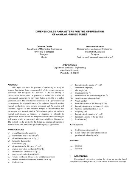
DIMENSSIONLES PARAMETERS FOR THE OPTIMIZATION
OF ANNULAR -FINNED TUBES
Cristóbal Cortés
Department of Mechanical Engineering
University of Zaragoza
Zaragoza
Spain.
Antonio Campo
Department of Nuclear Engineering
Idaho State University
Pocatello, ID, 83209
L’ dimensionless fin length, L’ = L/D
corrected fin length (m)
L c
Lt tube length (m)
m fin parameter (m – 1 )
nf number of fins per unit tube length (m – 1 )
Nu Nusselt number (dimensionless)
Pr Prandtl number
R thermal resistance of the fin array (K/W)
R’ dimensionless thermal resistance, R’ = RkLt
Re Reynolds number based on D and V
u fin spacing (m)
u’ dimensionless fin spacing, u’ = u/D
V free stream velocity of the gas (m/s)
Vf fin volume (m 3 )
Greek symbols
η f
fin efficiency (dimensionless)
ηt overall surface efficiency (dimensionless)
ν gas kinematic viscosity (m 2 /s)
Subscripts
min
opt
Inmaculada Arauzo
Department of Mechanical Engineering
University of Zaragoza
Zaragoza
Spain (e-mail: iarauzo@posta.unizar.es)
minimum
optimum
1 INTRODUCTION
Conventional engineering practice for sizing an annular-finned
compact heat exchanger makes use of surface efficiency relationships

combined with an experimental correlating equation for the average heat
transfer coefficient h on the finned surface. A good example of this
procedure can be found for instance in the classical text book of Kays
and London (1984a). The heat transfer literature offers many options
for the estimation of h, ranging from generic and easy-to-use formulae
which correlate the performance of a great variety of geometries
(Schmidt, 1963) to specific data for standard configurations, reported
in tabular or graphical form (Kays and London, 1984b).
As in many other branches of engineering, the traditional
approach naturally embodies strong simplifications. These have been
progressively recognized along the advancement of experimental and
numerical techniques. Due to the complexity of the flow induced by
the extended surface, a high lack of uniformity in the local convection
coefficient obtains, impairing the use of an average value (Schüz and
Kottke, 1992). Likewise, as a result of the modified velocity patterns,
a variable fin spacing leads to substantial changes in h that are not
completely predicted by the conventional correlations (Watel et al.,
1999).
The general design of extended surfaces is certainly an specialized
and complex matter, which requires expensive research tools, and
whose results often become the object of proprietary knowledge.
Nevertheless, for the modest objective of selecting and sizing the most
suitable annular-fin geometry, the traditional method may take
advantage of the recent developments in the field, at once retaining a
notable simplicity.
In particular, the variation of the correlated value of h raises the
question of the optimization of finned tube arrays. For a given volume
of fin material, the overall thermal resistance tends both to increase and
decrease with the fin spacing, due to the simultaneous increase of the
convective coefficient and decrease of the effective heat transfer area.
Assuming from the start that a reliable empirical fit for h is
available, this paper analyzes the problem from a theoretical and
practical perspective. Firstly, the optimization is stated in terms of
dimensional variables, deducing an implicit expression for the optimum
fin spacing. Then, a non-dimensional formula is proposed, resulting in
a remarkable simplification. The meaning of the corresponding
dimensionless groups is also very appropriate to the problem in hand.
A parametric study is subsequently undertaken for the usual
ranges of the main variables. The optimum is calculated by means of
standard numerical techniques. The results seem to be coherent, and
several interesting trends are pointed out. Finally, as a kind of
validation of the method, the classical geometries of annular-finned
tubes are examined in search of their optimum points of thermal
performance. The results are again fully satisfactory, showing that a
reasonable optimization was already present in the traditional designs.
D
u e
Lt
Figure 1. Geometry of an annular-finned tube.
2 PROBLEM STATEMENT
The problem is defined as the determination of the optimum
arrangement of an annular-finned tube for a fixed volume of fin
material. The optimum arrangement is the set of geometric parameters
in Fig. 1 that leads to a minimum value of the thermal resistance of the
fin array. The latter is expressed as
1
R =
hη A
t
where the overall surface efficiency η t and area calculations are
given by
Af
ηt = 1 − ( 1 − ηf
)
(2)
A
A
f
( 2 )
⎛ Lt
⎞
⎛ D + L − D
= π⎜
⎟⎜
⎝ u + e⎠⎜
⎝ 2
2 2
L
⎞
+ ( D + 2L)
e ⎟
⎠
⎛ u ⎞
A = π DLt⎜
⎟ + Af
(4)
⎝ u + e⎠
In Eq. (2), the fin efficiency η f can be calculated with the wellknown
results of 1D conduction theory. If a corrected length Lc = L +
e/2 is combined with the exact solution for an adiabatic tip, η f is
approximately independent of the Biot number, being a function of
only two variables: the fin diameter ratio 1 + 2L’ + e’, where L’ = L/D
and e’ = e/D are respectively the dimensionless fin length and
thickness, and the dimensionless group
mL
c
2h
⎛ e ⎞
= ⎜ L + ⎟
k e ⎝ 2 ⎠
w
In order to close the specification of R, an adequate correlation for
the average convection coefficient h is needed. The method of
optimization can be developed for any empirical formula; in this study,
we have selected a correlation recently reported in the literature (Watel
(1)
(3)
(5)

et al., 1999), valid for Pr ≈ 0.7:
k
h = Nu ; Nu = 0.446X Re (6)
D
0. 55
0. 55
e K
X
u u b
= + ′ ⎛ ⎞ ⎛
−0.
07 ⎞
⎜1
⎟ ⎜1
− ⋅ Re ⎟
(7)
⎝ ′ ⎠ ⎝ ′ ⎠
The Reynolds number Re = VD/ν is based on the tube diameter D
and the free stream velocity V. The validity range is 2550 ≤ Re ≤ 42
000. The dimensionless fin spacing is denoted u’ = u/D, and the
constants K and b are given for two separate ranges of this parameter:
K = 062 . , b = 0. 27⎫
⎧0034
. ≤ u ′ ≤ 014 .
⎬ for ⎨
(8)
K = 0. 36, b = 055 . ⎭ ⎩ 014 . ≤ u ′ ≤ 0. 69
To summarize, Eqs. (1)-(8) give the thermal resistance R as a
function of the following variables:
R = f (Re, k, kw, D, e, u, Lt, L) (9)
Therefore, the ensuing formal statement is as follows: Minimize
R, Eq. (9), for a fixed value of the fin volume
V
f
π Lt e
=
4 u + e
[ ( D + 2L)
− D ]
2 2 (10)
If we select the fin spacing u as the dependent variable and
eliminate the fin length L with V f , it follows that
u opt = f(Re, k, k w, D, e, L t, V f) (11)
the function f being implicitly described by all the foregoing equations
when evaluated at the minimum value of R.
3 DIMENSIONLESS VARIABLES
Equation (11) is clearly useless for a general study. Consequently,
we proceed to cast it in non-dimensional form. To this end, a new
dimensionless variable can be conceived in a rather contorted but
advantageous way. Suppose that all the material available is used to
build a hollow cylinder whose inner diameter is D, the outer diameter
of the tube. We may imagine it as the limit fin array that possess a
spacing u = 0, and thus designate its thickness as L u=0. Now define the
dimensionless coefficient k v > 1 as the diameter ratio of this imaginary
cylinder. The volume V f is accordingly
π
[ ( 2 = 0) ] ( 1)
2 2 2 2
π
Vf = Lt D + Lu − D = D Lt kv
−
4
4
(12)
from which we can obtain k v as
4V
f
kv = 1+ 2Lu′
= 0 = + 1 2
πD
L
or, equating Eqs. (10) and (12):
k
t
(13)
e′
= 1 + [( 1+ 2 L′
) −1]
(14)
u′ + e′
2 2
v
It is only a question of algebraic manipulations to use this
formula in Eqs. (3) and (4) in order to express the areas as
A DL kv
−
f = t
e′
+ ′ + ′
⎛
π ⎜
⎝ 2
2 1
( 1 2 )
e L ⎞
⎟
u ′ + e′
⎠
(15)
A DL kv
− L e
= t
e′
u e
+
′ ′
′ + ′ +
⎛ 2
1 2 ⎞
π ⎜
1 ⎟
(16)
⎝ 2
⎠
Finally, a dimensionless thermal resistance is defined multiplying
the specific value per unit tube length by the fluid thermal conductivity
k:
kLt
R′ = kLt R =
hη A
t
(17)
The resistance R’ is given by Eqs. (2), (5)-(8), (15) and (16). An
adequate inventory of the variables shows that the non-dimensional
form of Eq. (9) is then
kw
R′ = f (Re, , e′ , u′ , L′ , kv
) (18)
k
Now, as a consequence of the definition of the coefficient k v,
fixing a volume V f of fin material is equivalent to fixing a value of k v for
the same tube diameter D and length L t, Eq. (12). This statement
connects the optimization problem with the other aspects of heat
exchanger design, namely, the circulation of the inner fluid (D) and the
heat rating for the selected geometry (L t). If we eliminate the
dimensionless fin length L’ as a function of k v from Eq. (14), in view of
Eq. (18) we arrive at
kw
u′ opt = f (Re, , e′ , kv
) (19)
k
This expression can be regarded as the proper dimensionless form
of Eq. (11). In conclusion, the dependence of the optimum spacing on
four geometric parameters (D, e, Lt and Vf) has been reduced to uopt ′
being a function of only two: the dimensionless fin thickness e’ and the

volume coefficient k v.
4 PARAMETRIC STUDY
In order to demonstrate the advantages of the proposed method, a
parametric study has been undertaken for typical values of the
independent dimensionless variables. These are shown in Table 1. The
Reynolds numbers have been chosen in accordance with common
design practices for gas flow. The range of e’ is that found in standard
geometries of compact heat exchangers (Kays and London, 1984b).
The value at the base case coincides with the one experimentally tested
when deriving the correlation adopted for the convection coefficient
(Watel et al., 199). Three thermal conductivity ratios have been set
considering representative figures for the fin material (k w = 50, 100 and
150 W/m K) and air at 350 K (k = 0.03 W/m K).
The volume coefficient k v has been parametrized in 46 different
values, from k v = 1.05 to k v = 1.5, in steps of 0.01. Again, this range
widely covers the habitual design practices. The optimization has
proceed by minimizing the function R’ with u’ as the dependent
variable. The golden section search algorithm has been used, as
implemented in a commercial solver (Klein and Alvarado, 1992).. The
criteria of convergence was a relative error less than 0.1%.
Table 1. Dimensionless values for the parametric study
Re e’ k w/k
minimum 2 500 0.01 1 666
base case 10 000 0.017 3 333
maximum 40 000 0.047 5 000
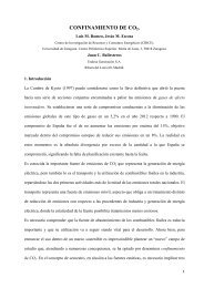
The results are shown graphically in Figs. 2, 3 and 4. In the first
place, Fig. 2 is a plot of the calculated minimum thermal resistance vs.
the volume coefficient, over the studied range of kv. Logically, Rmin ′ decreases with the volume, and the effect of the
optimization is more pronounced the less material is available.
The most influential parameter turns out to be the Reynolds
number, followed by the fin thickness. The latter means that there will
be several possibilities for optimizing a given situation. Limitations in
e’ dictated by the material or the manufacturing method will play an
important role. The effect of the ratio kw/k is very small, a fortunate
circumstance, since it is almost completely determined by the gas
temperatures and the fin material.
R' min
0.0035
0.0030
0.0025
0.0020
0.0015
0.0010
0.0005
104 0.017 3333 104 Re e' kw /k Re e' kw /k
0.017 1666
10 4 0. 010 3333
10 4 0.047 3333
104 0.017 5000
4.10 4 0.017 3333
2.5.10 3 0.017 3333
0.0000
1 1.1 1.2 1.3 1.4 1.5
kv Figure 2. Minimum value of R’ vs. k v.
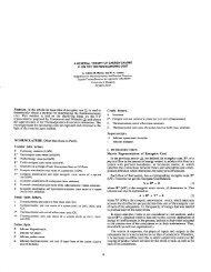
The graphs in Figs. 3 and 4 represent the variation of uopt ′ with kv for the base case and extreme values of e’ and Re, respectively. The
trends are very reasonable. For the same volume of fins, the optimum
spacing increases with their thickness and decreases with the Reynolds
number, since the latter allows a lower value of e’ with identical h. The
step in the curves is caused by the lack of continuity of the correlation
given by Eqs. (6)-(8) at u’ = 0.14. The asymptotic character of some
curves is also artificial, since the optimization was constrained within
the specified correlation range for the dimensionless thickness, Eq. (8).
0.7
u' opt
0.6
0.5
0.4
0.3
0.2
0.1
0
e' = 0.010
e '= 0.047 Re = 10 4
k w /k = 3333
e' = 0.017
1 1.1 1.2 1.3 1.4 1.5
kv

u' opt
0.7
0.6
0.5
0.4
0.3
0.2
0.1
Figure 3. Optimum spacing vs. kv and fin thickness.
0
Re = 2500
Re = 10000
Re = 40000
1 1.1 1.2 1.3 1.4 1.5
kv
e' = 0.017
kw /k = 3333
Figure 4. Optimum spacing vs. kv and Reynolds number.
5 RESULTS FOR STANDARD GEOMETRIES
The method of optimization has been applied to the geometries of
compact, annular-fined tubular heat exchangers whose thermal
performance data was compiled by Kays and London (1984b),
Table 2.

Table 2. Geometries of standard annular-finned tubes.
surface designation D (mm) L (mm) L’ e’ u’ n f (m –1 ) V f ·10 5 (m 3 ) k v
CF-7.34 9.650 6.86 0.711 0.0474 0.3105 289 4.708 1.28
CF-8.72 9.650 6.86 0.711 0.0474 0.2545 343 5.583 1.33
CF-8.72(c) 1.067 5.60 0.525 0.0448 0.2257 343 4.741 1.24
CF-11.46 9.650 6.86 0.711 0.0421 0.1876 451 6.520 1.38
CF-7.0-5/8J 1.638 6.05 0.369 0.0155 0.2060 276 2.981 1.07
CF-8.7-5/8J 1.638 6.05 0.369 0.0155 0.1626 343 3.708 1.08
CF-9.05-3/4J 1.966 8.75 0.445 0.0155 0.1273 356 8.481 1.13
CF-8.8-1.0J 2.601 9.05 0.348 0.0117 0.0993 346 10.530 1.09
First of all, our estimation after Watel et al. (1999) correlation of
the average convection coefficient has been confronted with the original
data, which essentially encompasses the same interval of Reynolds
numbers. Deviations in the value of Nu range from 5 to 15 %,
depending on Re and the geometry. This is deemed to be acceptable for
a general correlation formula. Curiously, the measurements in Watel et
al. (1999) are systematically higher than the values reported in by
Kays and London (1984b), in spite of the fact that the former refers to
a single tube and the latter to a tube bundle.
Figure 5 shows the curves uopt ′ vs. Re for the eight geometries
considered. The design value of u’ is indicated in the left ordinates. It
can be observed that each geometry becomes the optimum for a
Reynolds number that lies always within the expected range of
operation. Therefore, the proposed method seems to be coherent with
the traditional design procedures.
u' design
CF-7.34
CF-8.72
CF-11.46
CF-9.05-3/4J
CF-8.72(c)
CF-8.8-1.0J
CF-7.0-5/8J
CF-8.7-5/8J
u' opt
0.35
0.25
0.15
0 5000 10000 15000 20000 25000
0.05
30000 35000 40000
Re
Figure 5. Curves u’opt vs. Re for the geometries of Table 2.
0.3
0.2
0.1
6 CONCLUSIONS
A method of optimization of annular fin arrays has been
discussed, based on an original dimensionless form of the heat transfer
relationships, and a given empirical formula for the average convection
coefficient. The results are completely coherent and agree well with
standard fin geometries already optimized by the experience. It can be
useful in engineering design, as well as scaling-up, of compact heat
exchangers for gas-liquid or gas-gas applications.
A possible use of the method would consist in the following
sequence:
1 Determine the required value of R’ as dictated by the energy
balance and the heat transfer calculations, taking into account, if
relevant, the thermal resistance of the inner fluid and the possible
fouling.
2 From the values of V and D (as determined by flow and pressure
drop requirements), calculate Re.
3 Select the fin thickness and material, thus fixing the parameters e’
and k w/k.
4 With the aid of Fig 2., determine the minimum amount of material
needed to build the fin array with the prescribed value of R’.
5 A plot of the style of Fig. 3 or 4 for the adequate value of the
variables allows the determination of the fin spacing u’. Equation
(14) then gives the fin length L’.

7 REFERENCES
Kays, W. K., and London, A. L., 1984a, Compact Heat
Exchangers. Third Edition, McGraw-Hill, New York, 1984, chap. 2.
Kays, W. K., and London, A. L., 1984b, Compact Heat
Exchangers. Third Edition, McGraw-Hill, New York, 1984, chaps. 9
and 10.
Klein, S. A., and Alvarado, F. L., 1992, EES: Engineering
Equation Solver. Reference manual, F-Chart software, 1992, Appendix
B.
Schmidt, Th. E., 1963, “Der Wärmeübergang an Rippenrohren und
die Berechnung von Rohrbündel-Wärmeaustaus-chern”, Kältetechnik,
vol. 12, pp. 370-378, 1963.
Schüz, G. and Kottke, V., 1992 “Local Heat Transfer and Heat
Flux Distributions in Finned Tube Heat Exchangers”, Chem. Eng.
Technol., vol. 15, pp. 417-424, 1992.
Watel, B., Harmand, S., and Desmet, B., 1999 Influence of Flow
Velocity and Fin Spacing on the Forced Convective Heat Transfer from
an Annular-Finned Tube, JSME Int. J. Series B, vol. 42, pp. 56-64,
1999.