a truly multivariate approach to manova - Department of Psychology ...

Applied Multivariate Research, Volume 12, No. 3, 2007, 199-226. 

A TRULY MULTIVARIATE APPROACH TO MANOVA 

James W. Grice 

Oklahoma State University 

Michiko Iwasaki 

University of Washington School of Medicine 

ABSTRACT 

All too often researchers perform a Multivariate Analysis of Variance 

(MANOVA) on their data and then fail to fully recognize the true multivariate 

nature of their effects. The most common error is to follow the MANOVA with 

univariate analyses of the dependent variables. One reason for the occurrence of 

such errors is the lack of clear pedagogical materials for identifying and testing 

the multivariate effects from the analysis. The current paper consequently reviews 

the fundamental differences between MANOVA and univariate Analysis of 

Variance and then presents a coherent set of methods for plumbing the multivariate 

nature of a given data set. A completely worked example using genuine data 

is given along with estimates of effect sizes and confidence intervals, and an 

example results section following the technical writing style of the American 

Psychological Association is presented. A number of issues regarding the current 

methods are also discussed. 

INTRODUCTION 

Multivariate statistical methods have grown increasingly popular over the past 

twenty-five years. Most graduate programs in education and the social sciences 

now offer courses in multivariate methods. Statistical software such as SAS and 

SPSS that provide canned routines for conducting even the most complex multivariate 

analyses can also be found on the computers of modern educational researchers, 

psychologists, and sociologists, among other scientists. A wide array of 

multivariate textbooks written for both novices and experts can likewise be found 

on the bookshelves of these scientists. The continued proliferation of multivariate 

statistical procedures can no doubt be attributable to the belief that models of 

nature and human behavior must often account for multiple, inter-related variables 

that are conceptualized simultaneously or over time. Multivariate Analysis of 

Variance (or MANOVA) is one particular technique for analyzing such multivariable 

models. 

In MANOVA the goal is to maximally discriminate between two or more 

distinct groups on a linear combination of quantitative variables. For instance, a 

psychologist may wish to investigate how children educated in Catholic schools 

differ from children educated in public schools on a number of tests that measure: 

199

APPLIED MULTIVARIATE RESEARCH 

(1) reading, (2) mathematics, and (3) moral reasoning skills. Using MANOVA the 

psychologist could examine how the two groups differ on a linear combination of 

the three measures. Perhaps the Catholic school children score higher on moral 

reasoning skills relative to reading and math when compared to the public school 

children? Perhaps the Catholic school children score higher on both moral reasoning 

skills and math relative to reading when compared to the public school children? 

These potential outcomes, or questions, are multivariate in nature because 

they treat the quantitative measures simultaneously and recognize their potential 

inter-relatedness. The goal of conducting a MANOVA is thus to determine how 

quantitative variables can be combined to maximally discriminate between distinct 

groups of people, places, or things. As will be discussed below this goal also 

includes determining the theoretical or practical meaning of the derived linear 

combination⎯or combinations⎯of variables. 

Many excellent journal articles and book chapters have been devoted to 

MANOVA in the past twenty-five years. Chapters by Huberty and Petoskey 

(2000) and Weinfurt (1995), for instance, provide lucid introductions to this 

complex and conceptually powerful statistical procedure. Multivariate textbooks 

by Stevens (2001), Tabachnick and Fidell (2006), and Hair, et al. (2006), to name 

a few, also provide outstanding treatments of MANOVA. Despite these resources, 

however, a central premise of the current paper is that many published applications 

of MANOVA fail to exploit the conceptual advantage of conducting a 

multivariate, rather than univariate, analysis. Recent reviews (Huberty & Morris, 

1989; Keselman, et al., 1998; Kieffer, Reese, & Thompson, 2001), for instance, 

have shown that studies employing MANOVA to explore group differences on 

multiple quantitative variables often fail to realize the multivariate nature of the 

reported effects. Instead, authors tend to resort to ‘‘follow-up’’ univariate statistical 

analyses to make sense of their findings (viz., following a significant 

MANOVA with multiple ANOVAs). One potential reason for these bad habits of 

data analysis is a paucity of clear examples that demonstrate appropriate procedures. 

Consequently, we draw upon the work of Richard J. Harris (1993, 2001; 

Harris, M., Harris, R., & Bochner, 1982) and Carl J. Huberty (Huberty, 1984; 

Huberty & Smith, 1982; Huberty & Petoskey, 2000; also, see Enders, 2003) in the 

current paper to demonstrate a general strategy for conducting MANOVA. This 

strategy focuses on the linear combinations of variables, or multivariate composites, 

that are the numerical and conceptual basis of any multivariate analysis; 

subsequently, specific techniques for identifying and testing these composites for 

statistical significance will be shown. An approach for interpreting and labeling 

the multivariate composites will also be presented, and an example write-up of 

MANOVA results that follows APA style will be provided. 

MANOVA vs. ANOVA 

Simply defined, MANOVA is the multivariate generalization of univariate 

ANOVA. In the latter analysis mean differences between two or more groups are 

examined on a single measure. For instance, a psychologist may wish to study the 

mean differences of ethnic groups on a continuous measure of implicit racism, or 

an educator may wish to examine the differences between boys and girls regarding 

their mean performance on a test of mathematical reasoning ability. In comparison, 

and as stated above, the goal in MANOVA is to examine mean differ- 

200

MULTIVARIATE ANALYSIS OF VARIANCE 

ences on linear combinations of multiple quantitative variables. Ethnic groups, 

for instance, could be compared on a combination of explicit and implicit measures 

of racism, or boys and girls could be compared with regard to their mean 

performances on a combination of mathematical, spatial, and verbal reasoning 

tasks. In both instances the variables would be analyzed simultaneously (i.e., 

multivariately) rather than individually (i.e., univariately). 

Because the differences between these univariate and multivariate procedures 

can best be explicated by way of example, we will proceed with a complete 

analysis of genuine data. Specifically, we will draw data from a Master’s thesis 

by Iwasaki (1998) in which the personality traits of different cultural groups were 

examined. 1 In addition to other measures, college students in Iwasaki’s study 

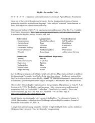
completed the NEO PI-r (Costa & McCrae, 1992), a popular questionnaire that 

measures the Big Five personality traits: Neuroticism, Extraversion, Openness-to- 

Experience, Agreeableness, and Conscientiousness. The students were also classified 

into three groups: 

EA: European Americans (Caucasians living in the United States their 

entire lives) 

AA: Asian Americans (Asians living in the United States since before the 

age of 6 years) 

AI: Asian Internationals (Asians who moved to the United States after their 

6 th birthday) 

The three groups form mutually exclusive categories, and the personality questionnaire 

yields quasi-continuous trait scores (viz., they may range in value from 

0 to 192) that are assumed to represent an interval scale. The categorical grouping 

variable will herein be referred to as the independent variable, and the quasicontinuous 

trait measures will be referred to as the dependent variables. Note this 

terminology will be used throughout solely for the sake of convenience and is not 

intended to imply a causal ordering of the variables. As is well known, attributing 

cause is a logical and theoretical task that extends beyond the bounds of statistical 

analysis. 

The goal in univariate ANOVA is to examine differences in group means on a 

single, continuous variable. Therefore each dependent variable (Big Five trait 

score) is analyzed and interpreted separately. The results for the univariate tests of 

overall differences among the EA, AA, and AI groups from the SPSS MANOVA 

procedure (which can also be used to conduct ANOVAs) are as follows: 

EFFECT .. GRP 

Univariate F-tests with (2,200) D. F. 

Var Hypo. SS Error SS Hypo. MS Error MS F Sig. F eta-sqr 

Neu 456.85 90650.37 228.43 453.25 .50 .605 .01 

Ext 12180.69 68087.41 6090.35 340.44 17.89 .000 .15 

Ope 8773.97 58283.59 4386.99 291.42 15.05 .000 .13 

Agr 6550.10 61033.79 3275.05 305.17 10.73 .000 .10 

Con 1297.48 68134.10 648.74 340.67 1.90 .152 .02 

201


Using a Bonferroni adjusted a priori p-value of .01 (.05/5), the population means 

for the three groups are judged to be unequal on the extraversion, openness-toexperience, 

and agreeableness traits. The largest univariate effect is noted for 

extraversion, for which 15% (η 2 = .15) of the variability in the extraversion trait 

scores can be explained by group membership. This effect seems small, although 

it could be judged as large using Cohen’s (1988) conventions (.01 = small, .06 = 

medium, .14 = large). It should also be noted the homogeneity of population 

variances assumption was tested for each analysis and no violations were noted. 

Each of the statistically significant univariate, omnibus effects could be followed 

by complex or paired comparisons to clarify the nature of the mean differences 

between the EA, AA, and AI groups. The results from such analyses would 

be interpreted separately for each of the Big Five trait scores because the univariate 

approach essentially treats any potential correlations among the dependent 

variables as meaningless. 

By comparison a multivariate approach takes into account the inter-correlations 

among the Big Five personality traits. As can be seen in the following SPSS 

CORRELATION output, a number of the trait scores are modestly correlated: 

Correlations 

Agreeable- Conscien- 

Neuroticism Extraversion Openness ness tiousness 

Neuroticism 1.000 -.255** -.019 -.097 -.397** 

Extraversion -.255** 1.000 .363** .011 .371** 

Openness -.019 .353** 1.000 .232** .125 

Agreeableness -.097 .011 .232** 1.000 .097 

Conscientiousness -.397** .371** .125 .097 1.000 

** Correlation is significant at the 0.01 level (2-tailed) 

Reasoning multivariately with the same data, the question becomes: In what way 

or ways can the Big Five traits be combined to discriminate among the three 

groups? Perhaps a combination of high extraversion and low neuroticism separates 

the groups, or perhaps a combination of high extraversion, high agreeableness, 

and low conscientiousness discriminates among the three groups? These 

questions demonstrate how a multivariate frame of mind entails considering the 

dependent variables simultaneously rather than separately. Whether or not such 

questions are justified or meaningful is an issue that must be addressed by any 

researcher confronted with the prospect of conducting a MANOVA. In the current 

example this issue manifests itself as follows: Are we truly interested in examining 

the multivariate, linear combinations of Big Five traits, or are we content with 

considering each trait separately? Another way of considering the issue regards 

the intent to interpret the multivariate effect that might underlie the data. For the 

current example, if we have no intention of interpreting the multivariate composites 

(that is, the linear combinations of traits ⎯ the dependent variables), then the 

univariate analyses above are perfectly sufficient. There is certainly no shame in 

202


conducting multiple ANOVAs and separately interpreting the results for each 

dependent variable. It is more than a methodological faux pas, however, to 

conduct a MANOVA with no intent of interpreting the multivariate combination 

of variables. 

In fact, two common errors seem to be associated with the failure to accurately 

discriminate between univariate and multivariate approaches toward data analysis. 

First, many researchers believe that conducting a MANOVA will provide 

protection from Type I error inflation when conducting multiple univariate 

ANOVAs. Following this erroneous reasoning, for instance, we would first 

conduct a MANOVA for the personality data above and, if significant, judge the 

statistical significance of the univariate ANOVAs based on their unadjusted 

observed p-values rather than their Bonferroni-adjusted p-values. Although such 

an analysis strategy is common in the literature, it is not to be recommended 

because the Type I error rate will only be properly controlled when the null 

hypothesis is true (Bray & Maxwell, 1982), which is an unlikely occurrence in 

practice and therefore an unrealistic assumption. Type I error inflation can be 

controlled through the use of a Bonferroni adjustment or a fully post hoc critical 

value derived from the results of a MANOVA, but the researcher must make the 

extra effort to compute the critical values against which to judge each univariate 

F-test (see Harris, 2001, and below). To reiterate, simply running a MANOVA 

prior to multiple ANOVAs will not generally provide appropriate protection 

against Type I error inflation. The extra step of computing the Bonferroni-adjusted 

critical values or the special MANOVA-based post hoc critical value must also 

be taken. 

Second, many researchers believe that ANOVA should be used as a follow-up 

procedure to MANOVA for interpreting and understanding the multivariate effect. 

While common, this analysis strategy is based on the misconception that 

results from multivariate analyses are simply additive functions of the results 

from univariate analyses. As will be described below, however, the multivariate 

information from a MANOVA is contained in the linear combinations of dependent 

variables that are generated from the analysis. Conducting an ANOVA on 

each of the dependent variables following a MANOVA completely ignores these 

linear combinations. Furthermore, the conceptual meaning of the results from a 

series of ANOVAs will not necessarily match the conceptual meaning of the 

results from a MANOVA. In other words, the multivariate nature of the results 

will not necessarily emerge from a series of univariate analyses. Techniques for 

identifying and exploring the linear combinations of variables that result from a 

MANOVA are therefore of critical importance. 

CONDUCTING THE MANOVA 

Returning to the Big Five trait example, let us decide to pursue a truly multivariate 

approach. In other words, let us commit to examining the linear combinations 

of personality traits that might differentiate between the European American 

(EA), Asian American (AA), and Asian International (AI) students. Assuming 

that no a priori model for combining the Big Five traits is available, these six 

steps will consequently be followed: 

203


1. Conduct an omnibus test of differences among the three groups on 

linear combinations of the five personality traits. 

2. Examine the linear combinations of personality traits embodied in the 

discriminant functions. 

3. Simplify and interpret the strongest linear combination. 

4. Test the simplified linear combination (multivariate composite) for 

statistical significance. 

5. Conduct follow-up tests of group differences on the simplified multivariate 

composite. 

6. Summarize results in APA style 

If an existing model for combining the traits were available, a priori, then an 

abbreviated approach, which will be discussed near the end of this paper, would 

be undertaken. 

Step 1: Conducting the Omnibus MANOVA. 

The omnibus null hypothesis for this example posits the EA, AA, and AI 

groups are equal with regard to their population means on any and all linear 

combinations of the Big Five personality traits. This hypothesis can be tested 

using any one of the major computer software packages. In SPSS for Windows 

the General Linear Model (GLM) procedure can be used or the dated MANOVA 

routine can be run through the syntax editor. There are several slight advantages 

to using the MANOVA syntax; consequently these procedures are employed 

herein, and the complete annotated syntax statements can be found in the Appendix. 

The multivariate results from SPSS MANOVA are: 

EFFECT .. GRP 

Multivariate Tests of Significance (S = 2, M = 1 , N = 97 ) 

Test Name Value Approx. F Hypoth. DF Error DF Sig. F 

Pillais .41862 10.42982 10.00 394.00 .000 

Hotellings .53723 10.47592 10.00 390.00 .000 

Wilks .62327 10.45320 10.00 392.00 .000 

Roys .25313 

Note.. F statistic for WILKS’ Lambda is exact. 

As can be seen, four test statistics are reported for the group effect: ‘‘Pillais’’, 

‘‘Hotellings’’, ‘‘Wilks’’, and ‘‘Roys.’’ Huberty (1994, pp. 183-189) offers a 

detailed discussion of these four statistics, and the first three tests indicate the 

multivariate effect is statistically significant for the current data (all ‘Sig. F’ 

values, that is, p’s < .001). Wilks’ Lambda is arguably the most popular multivariate 

statistic, and Tabachnik and Fidell (2006) generally support reporting it instead 

of the other values. 

The analysis strategy recommended in this paper, however, employs Roy’s 

g.c.r. A number of details regarding this statistic must therefore be clarified. First, 

it is often reported in two different metrics. In the SPSS output shown above, 

204


which was generated with the MANOVA routine, it is reported as a measure of 

association strength, θ = .25, that indicates the proportion of overlapping variance 

between the independent variable and the first linear combination of dependent 

variables. In other words, θ is equivalent to the well-known η 2 measure of association 

strength. SPSS output generated from the GLM option in the pull-down 

menus appears in a different format: 

Multivariate Tests c 

Effect Value F Hypotheses df Error df Sig. 

Intercept Pillai’s Trace .995 7270.287 a 

Wilk’s Lambda .005 7270.287 a 

Hotelling’s Trace 185.466 7270.287 a 

Roy’s Largest Root 185.466 7270.287 a 

205 

5.000 196.000 .000 

5.000 196.000 .000 

5.000 196.000 .000 

5.000 196.000 .000 

GRP Pillai’s Trave .419 10.430 10.000 394.000 .000 

Wilk’s Lambda .623 10.453 a 

10.000 392.000 .000 

Hotelling’s Trace .537 10.476 10.000 390.000 .000 

Roy’s Largest Root .339 13.354 b 

5.000 197.000 .000 

a. Exact statistic 

b. The statistic is an upper bound on F that yields a lower bound on the significance level. 

c. Design: Intercept + GRP 

As can be seen, except for ‘‘Roy’s Largest Root’’, the test values are equal to 

those generated by the MANOVA routine. The value for Roy’s g.c.r. from GLM 

is reported as an eigenvalue (λ = .34) which can be easily computed from the θ 

value: 

λ = 

θ 

, θ = 

1 − θ 

λ 

1 + λ 

When using a program other than SPSS, the researcher should be certain to explore 

the software manuals to determine which metric is being reported. Alternatively, 

as will be shown in the next step in the procedures, the value of θ can be 

computed ‘‘manually’’ with compute statements. 

The second issue regarding Roy’s g.c.r. is the F-value and hypothesis test 

generated by the GLM procedure. This test is an upper bound that may unfortunately 

lead to dramatically high Type I error rates (Harris, personal communication, 

October 26 th , 2005). It should consequently be avoided, and the tabled 

values for θ reported by Harris (1985, 2001) should instead be used. A program 

reported by Harris (1985, p. 475) can also be used to compute the observed pvalue 

for Roy’s g.c.r. (in the θ metric) with s, m, and n degrees of freedom. 2 

These values are computed as: 

s = min(df effect, p) 

m = (⏐df effect - p⏐ - 1) / 2 

n = (df error - p - 1) / 2

where, 


p = number of dependent variables 

df effect = k - 1 

df error = N - k 

N = number of observations 

k = number of groups 

For the current data p = 5, k = 3, and N = 203. Consequently, df effect = 2, df error = 

200, s = min(2,5) = 2, m = (⏐2 - 5⏐ - 1) / 2 = 1, and n = (200 - 5 - 1) / 2 = 97 as 

reported in the MANOVA output above. Harris’ program yields a critical θ value 

(θ crit ) of .07056 for a critical p-value (p crit ) of .05. The observed θ of .25313 

exceeds θ crit and is therefore statistically significant. Entering various p-values 

through trial-and-error in Harris’ program reveals the observed p-value to be less 

than .0005. 

Finally, now that Roy’s statistic has been explained, the other omnibus tests of 

the multivariate effect can be succinctly described for pedagogical purposes as 

follows: 

Pillai’s Trace is the sum of the effect sizes for the discriminant functions; 

that is, Σθ i . A value approaching s indicates a large omnibus effect, and 

when s = 1 Pillai’s Trace will equal Roy’s θ. 

Hotelling’s Trace is similar to Pillai’s Trace, but is based on eigenvalues; 

namely, Σλ i . The magnitude of Hotelling’s Trace is difficult to interpret 

since it has no set range, although when s = 1 the result will equal Roy’s λ. 

Wilks’ Lambda (Λ) is based on overlapping variances, or effect sizes, 

namely, Π(1−θ i ). Opposite of the other test statistics, values near 0 indicate 

large omnibus effects. 

These three tests differ from Roy’s test by combining, in some manner, the 

information for all the discriminant functions produced from the analysis for a 

given effect. 

Step 2: Examining the Linear Combinations 

As was stated at various points above the multivariate effect is conveyed 

through the linear combinations of Big Five traits. These linear combinations are 

defined by the discriminant function coefficients that can be requested from most 

computer programs in both raw and standardized form. The coefficients from 

SPSS MANOVA for the current example are reported as follows: 

206


EFFECT .. GRP (Cont.) 

Raw discriminant function coefficients 

Function No. 

Variable 1 2 

N -.00580 -.00700 

E -.06027 -.00017 

O .04239 -.04230 

A -.02758 -.03102 

C .00748 -.00956 

Standardized discriminant function coefficients 

Function No. 

Variable 1 2 

N -.12356 -.14893 

E -1.11200 -.00309 

O .72369 -.72218 

A -.48180 -.54193 

C .13811 -.17640 

The discriminant function coefficients are regression weights that are multiplied 

by the Big Five scale scores (N, E, O, A, C) in original or z-score units to create 

the multivariate composites referred to throughout this manuscript. Consequently, 

these regression weights are the heart and soul of MANOVA because they represent 

exactly how the dependent variables are combined to maximally discriminate 

between the EA, AA, and AI groups. Depending on the number of groups and the 

number of dependent variables, one or more linear combinations, or multivariate 

composites, will be generated. The value of s degrees of freedom will in fact 

indicate the number of multivariate composites produced. In the current example, 

two composites are produced based on the three groups and five personality traits. 

These two composites are furthermore uncorrelated (orthogonal) and ordered in 

terms of their ‘‘strength’’; that is, the extent to which they overlap with the independent 

variable. 

Using the unstandardized coefficients above, the first multivariate composite 

can be written and computed as follows: 

Composite #1 = (N)(-.0058) + (E)(-.06027) + (O)(.04239) + (A)(-.02758) + 

(C)(.00748). 

This new variable can be entered as a single dependent variable in an 

ANOVA, yielding the following results: 

Source of Variation SS DF MS F Sig of F 

WITHIN CELLS 200.01 200 1.00 

GRP 67.79 2 33.89 33.89 .000 

(Total) 267.80 202 1.33 

207


A measure of association strength between the independent variable and multivariate 

composite, η 2 , can then be computed: 

(F observed )(df between ) (33.89)(2) 

η2 = = = .25 

(Fobserved )(dfbetween ) + df (33.89)(2) + 200 

within 

The result, .25, is equal to Roy’s g.c.r. reported above as θ. Computing the 

multivariate composite and conducting an ANOVA thus demonstrates that Roy’s 

g.c.r. is a measure of effect size for the first linear composite. The second multivariate 

composite is orthogonal to (i.e., uncorrelated with) the first and can be 

written and computed as follows: 

Composite #2 = (N)(-.007) + (E)(-.00017) + (O)(-.0423) + (A)(-.03102) + 

(C)(-.00956). Conducting an ANOVA and computing η 2 yields: 


WITHIN CELLS 199.88 200 1.00 

GRP 39.64 2 19.82 19.83 .000 

(Total) 239.52 202 1.19 

(F observed )(df between ) (19.83)(2) 

η2 = = = .17 

(Fobserved )(dfbetween ) + df (19.83)(2) + 200 

within 

As mentioned above, the strength of association for this second composite is 

lower than the first. Nonetheless, it too can be tested for statistical significance 

using the same m and n degrees of freedom for testing the first composite, but s = 

min(k - j, p - j + 1), where j is equal to the composite’s ordinal value. In this case 

the second composite (j = 2) is being tested for statistical significance, and s = 

min(3 - 2, 5 - 2 + 1) = 1, and θ crit = .04702 for p crit = .05. The second composite is 

therefore also statistically significant since .17 > .04702. It is also noteworthy that 

the sum of the η 2 values for the first (.25) and second (.17) composites equals .42, 

which is the value for the Pillai’s Trace multivariate statistic above. Pillai’s Trace 

thus differs from Roy’s g.c.r. by testing group differences on the complete set of 

linear combinations generated from the analysis. Wilks’ Lambda and Hotelling’s 

Trace similarly provide tests of the complete set of multivariate composites. The 

omnibus nature of these three tests is a distinct disadvantage in the current approach, 

however, which focuses on testing and interpreting the individual discriminant 

functions. 

Step 3: Simplifying and Interpreting the First Linear Combination 

The next step in the analysis involves interpreting the multivariate composites 

defined by the discriminant functions. As was noted above, the first composite 

will always yield the highest θ (i.e., η 2 ) value, and in many genuine data sets the 

remaining composites can be ignored because of their small effect sizes. The 

second composite in the current example, however, shares 17% of its variance 

with the independent variable, which is nearly as high as the percentage for the 

first composite (25%). Nonetheless, solely for the sake of convenience, we will 

simplify and interpret only the first composite for the personality data. 

208


It is often useful to determine the ‘‘multivariate gain’’ of the composite under 

consideration over the univariate approach toward the same data. The gain is 

determined by comparing the θ value for the composite to the corresponding 

values from the univariate F-tests. For the current data the largest univariate η 2 

value was .15 for Extraversion, which is modestly lower than .25 for the first 

multivariate composite. The multivariate gain over simple univariate analyses 

was thus .10; in other words, the multivariate effect was 10 percentage points 

higher than the strongest univariate effect in terms of shared variance. 

As with any estimate of effect size the researcher must draw upon his or her 

experience and theoretical framework as well as existing literature to judge the 

importance of the multivariate gain. This judgement will also go hand-in-hand 

with the conceptual interpretation or labeling of the multivariate composite. The 

reader is most likely familiar with the process of interpreting and labeling multivariate 

composites in the realm of Exploratory Factor Analysis (EFA). In EFA 

one begins with a pool of items and attempts to identify a set of common factors 

believed to represent theoretically meaningful constructs (e.g., personality traits, 

clinical syndromes, dimensions of intelligence, etc.) that underlie the original 

items. Through a process of examining pattern, structure, or factor score coefficients 

the factors are ‘‘interpreted’’, which is to say they are labeled or named. 

The factors themselves are mathematically determined as multivariate functions 

of the original items in the analysis and are thus similar to the discriminant functions 

in MANOVA. Consequently, the methods commonly employed to interpret 

factors can be used to interpret multivariate composites. In factor analysis, for 

example, an arbitrary criterion is often used (e.g., ⏐.30⏐, ⏐.40⏐) to judge pattern 

or structure coefficients so that ‘‘salient’’ items may be identified for a given 

factor. Once the salient items are identified, their content is examined for a 

common theme which is then named and used as the factor label. 

In MANOVA this process of labeling should begin with an examination of 

simplified versions of the discriminant function coefficients. If the dependent 

variables are on different scales the standardized function coefficients and standardized 

variables (z-scores) should be used when interpreting and computing the 

simplified composite variable. If the dependent variables are all on the same 

scale, as in the current data, the raw (i.e., unstandardized) coefficients and raw 

scores should be preferred. The first composite is thus simplified by focusing only 

on the relatively large raw discriminant function coefficients. The full function is 

repeated here: 

Composite #1 = (N)(-.0058) + (E)(-.06027) + (O)(.04239) + (A)(-.02758) + 

(C)(.00748). Clearly, the coefficients for Neuroticism and Conscientiousness are 

relatively small and near zero. Converting these small coefficients to zero yields: 

Simplified Composite #1 = (N)(0) + (E)(-.06027) + (O)(.04239) + 

(A)(-.02758) + (C)(0). As is done in interpreting factors differences between the 

relatively large function coefficients are ignored. In other words, the coefficients 

are changed to unity while their signs are retained: 

Simplified Composite #1 = (E)(-1) + (O)(1) + (A)(-1) = O - (E + A). The 

rationale behind this simplifying process is to round to zero those coefficients that 

are relatively small because they are assumed to be deviating from zero well 

within the bounds of sampling variability (Einhorn & Hogarth, 1975; Grice, 2001; 

Wainer, 1976), although no statistical test of this assumption exists. Furthermore, 

209


the differences among the large coefficients are assumed to be within the bounds 

of sampling variability, and thus important information is not lost by converting 

these values to 1s and -1s consistent with their original signs (see Rozeboom, 

1979, for further discussion of this topic). Again, this is the same process used 

when interpreting factors in factor analysis, when creating sum scores from a 

factor analysis or multiple regression analysis, and generating contrast coefficients 

in analysis of variance from an examination of means. 

In words then, the multivariate composite that discriminates between the 

European American, Asian American, and Asian International students is higher 

Openness-to-Experience relative to lower Extraversion and Agreeableness. A 

sensible label to apply to this novel multivariate composite is ‘‘Reserved-Openness.’’ 

Individuals who score high on this composite are quietly or reservedly 

open to new experiences, whereas individuals who score low on this composite 

can be described as gregariously traditional (i.e., extraverted, agreeable, and low 

on openness). The composite can thus be interpreted as Reserved-Openness vs. 

Gregarious-Traditionalism. 

The nature of this multivariate composite can further be understood by examining 

the means in Figure 1. As can be seen in the highlighted (i.e., the ‘‘boxed’’) 

portions of the graph European Americans rate themselves higher on Extraversion 

and Agreeableness relative to Openness-to-Experience, whereas Asian Americans 

and Asian Internationals rate themselves higher on Openness-to-Experience relative 

to Extraversion and Agreeableness. It is thus the pattern of means, or more 

specifically the differences in patterns of means, that is captured by the simplified, 

multivariate composite. When reporting the results of the analyses for this 

particular study, the multivariate effect could possibly be discussed with respect 

to cultural differences between Asian and Caucasian Americans in terms of their 

personality types. Types, in the realm of personality psychology, are considered 

to be multivariate clusters of traits or other stable personal characteristics. 

The simplification and interpretation process is perhaps the most important 

stage of the MANOVA since it provides the bridge from a purely statistical effect 

to a theoretically meaningful effect. If at this point in the analysis the multivariate 

composite (i.e., the discriminant function) can not be labeled or theoretically 

interpreted, a switch to separate univariate analyses would be prudent. Otherwise, 

the researcher will be faced with a situation in which the multivariate effect is 

potentially large and statistically significant, but conceptually meaningless. 

Because of the importance of interpretation in the current approach toward 

MANOVA, a number of pointers for interpreting the multivariate function will be 

presented below. 

Step 4: Testing the Simplified Multivariate Composite for Statistical Significance. 

Do the EA, AA, and AI groups differ significantly in their means on the simplified 

composite, Reserved-Openness? Recall the three groups differed significantly 

on the full composite, as indicated by the Roy’s g.c.r. test (θ = .25, p 

< .0005). The mathematics underlying MANOVA will insure the θ values are 

maximized for each of the linear combinations of dependent variables, subject to 

the condition that each is uncorrelated with preceding discriminant functions. The 

multivariate composite produced from the simplification process is essentially a 

210


crude approximation of the first exact discriminant function, and it will always 

yield a lower θ value that must be tested for statistical significance. The formula 

can be found in Harris (2001, p. 222): 

df error θ crit 

F crit = (1 - θcrit ) df effect 

Using Harris’ g.c.r. program, θ crit = .0706 for s = 2, m = 1, n = 97, and p crit 

= .05. 



= (200)(.0706) 

(1-.0706)(2) 

211 

= 7.60 

The simplified composite, Reserved-Openness, can be computed in SPSS and 

entered as the dependent variable in an ANOVA: 


WITHIN CELLS 104562.38 200 522.81 

GRP 28955.74 2 14477.87 27.69 .000 

(Total) 133518.12 202 660.98 

R-Squared = .217 Adjusted R-Squared = .209 

The observed F-statistic (F obs = 27.69) exceeds F crit = 7.60 and is therefore statistically 

significant. The results consequently indicate the three EA, AA, and AI 

groups differ in terms of their population means on the multivariate composite 

Reserved-Openness. Moreover, the η 2 value is .22, which compares favorably 

to .25 for the full composite. The multivariate gain of the simplified composite 

(.15 compared to .22) is still substantial and similar to the multivariate gain of the 

full composite (.15 compared to .25). In other words, very little overlapping 

variance with the independent variable was lost in the simplification process. 

The direction of this effect can be understood by first computing the range of 

values that are possible on the simplified composite. The original scores on the 

Big Five scales could range in value from 0 to 192. The lowest possible score for 

Reserved-Openness is therefore -384 [viz., 0 - (192 + 192)], and the highest 

possible score is equal to 192 [viz., 192 - (0 + 0)]. The European Americans (M = 

-129.67, SD = 21.85) scored approximately 24 scale points lower, on average, 

than the Asian American (M = -107.68, SD = 26.03) and Asian International (M = 

-103.25, SD = 21.21) students on the Reserved-Openness composite. On a 576point 

scale, this average difference seems to reflect a modest, or small, effect size. 

On the other hand, the observed scores on the Reserved-Openness composite 

ranged from -179 to -28 for all 203 participants. Compared to this observed range, 

the approximate 24-point mean difference might be interpreted as more theoretically 

or practically significant. 

Step 5: Conducting Follow-up Tests on the Simplified Multivariate Composite. 

As in univariate ANOVA, an omnibus multivariate effect for three or more 

groups should be followed by pairwise comparisons or tests of complex contrasts.


Moreover, in univariate ANOVA the choice of an adjustment procedure (e.g., 

Tukey’s HSD, or Scheffe’) for controlling the Type I error rate will depend on 

two factors: (1) the type of contrasts, pairwise or complex; and (2) whether the 

contrasts are planned or constructed after examining the results. The same factors 

must be considered in MANOVA when contrasting the groups on the simplified 

multivariate composite. Additionally, one must consider whether the simplified 

multivariate composite was planned or constructed after examining the discriminant 

function coefficients. 

In the current example of Iwasaki’s personality data, the multivariate composite 

Reserved-Openness was constructed in a purely post hoc fashion. Let us 

further investigate, post hoc, a complex contrast and pairwise comparisons 

between the EA, AA, and AI groups. The complex contrast entails a comparison 

of the average AA and AI means with the EA multivariate composite mean [viz., 

(1)(AA) + (1)(AI) - (2)(EA)]. 3 Given the fully post hoc nature of the multivariate 

composite and the follow-up tests, Harris (2001) recommends a Scheffe’-style 

adjustment equal to the product of the g.c.r.-based F crit value above and df effect : 

(7.60)(2) = 15.20. This adjustment is admittedly conservative, but it is the price 

that must be paid when a priori theory is not available for constructing the multivariate 

composite or the group contrasts. More will be said about adjustments for 

Type I error rates below. 

For the current data the results for the complex comparison and all possible 

pairwise comparisons on the simplified composite (‘‘Comp 1’’) generated from 

SPSS GLM appear as follows: 

Contrast Coefficients 

212 

Group 

European Asian Asian 

Contrast Americans Internationals Americans 

1 -1 .5 .5 

2 -1 1 0 

3 -1 0 1 

4 0 -1 1 

Contrast Tests 

Value of 

Contrast Contrast Std. Error t df Sig. (2-tailed) 

Reserved-Openness Assume equal 1 24.2024 3.3347 7.258 200 .000 

variances 2 26.4167 3.7725 7.002 200 .000 

3 21.9881 4.0382 5.445 200 .000 

4 -4.4286 4.0740 -1.087 200 .278 

Does not assume 1 24.2024 3.3100 7.312 160.290 .000 

equal variances 2 26.4167 3.5520 7.437 144.982 .000 

3 21.9881 4.2978 5.116 106.810 .000 

4 -4.4286 4.2838 -1.034 104.810 .304


The tests for the contrasts are reported as t-values and must therefore be compared 

to the square root of 15.20, which equals 3.90 (t 2 = F for single degree of 

freedom contrasts). The results clearly show the European Americans are distinct 

from the Asian Americans and Asian Internationals on the multivariate composite. 

Specifically, the European Americans scored lower, on average, than the 

Asian International and Asian American students on the Reserved-Openness 

composite. The population means for the Asian groups were concluded to be 

equal. 

Given the American Psychological Association’s recent efforts (Wilkinson, et 

al., 1999) to encourage researchers to compute and report estimates of effect size 

as well as confidence intervals, these statistics should be derived and interpreted 

for the follow-up contrasts as well. As demonstrated above θ is a measure of 

association strength that can be reported as an indicator of the magnitude of effect. 

Similarly, η 2 values can easily be computed for the t-values obtained from 

the contrasts using the well-known formulae: 

η 2 

contrast 

t 2 

contrast 

213 

F contrast 

= = 

t 2 

contrast + df error F contrast + df error 

The η 2 result for the complex comparison, for instance, is .21 and indicates a 

large effect using Cohen’s conventions. 

Computing confidence intervals for contrasts of means on the simplified 

multivariate composite is more difficult and may require a modicum of matrix 

algebra (see Harris, 2001, p. 221). The confidence interval must take into account 

the contrast coefficients, the weights used to create the multivariate composite, 

and the matrix of residuals from the MANOVA. Specifically, the formula for a 

multivariate contrast is as follows: 

c 2 

j 

cXa' ± Σ (aEa')λ crit 

nj 

where c is a row vector of k contrast coefficients, a is a row vector of p weights 

used to define the multivariate composite, × is a k × p matrix of group means on 

the dependent variables, E is a p × p matrix of residuals (i.e., the error matrix 

from MANOVA), and λ crit is transformed from the θ crit value used for the omnibus 

test. The c j ’s and n j ’s are the contrast coefficients and sample sizes for the 

groups, respectively. 

Fortunately, as pointed out by a reviewer of this manuscript, the equation 

above can be simplified so that computing confidence intervals is a manageable 

task: 

Value of Contrast ± std. error (df error ) λ crit , 

where ‘Value of Contrast’, ‘std. error’, and df error are taken from the SPSS 

‘Contrast Tests’ table above (24.2024, 3.3347, and 200, respectively) for the first 

contrast. Using θ crit (.0706) from above,

Thus, 


θ crit 

λ crit = 1 - θcrit 

= (.0706) 

(1-.0706) 

24.2042 ± 3.3347 (200)(.0760) , 

214 

= .0760 

and the 95% confidence interval for contrasting the EAs with the Aas and Ais on 

the Reserved-Openness multivariate composite can be written as: 

11.20 < μ Comp(AA,AI) - μ Comp(EA) < 37.20. 

The center of the confidence interval is located at 24.20, the mean difference 

between the EA and averaged AA and AI groups on the Reserved-Openness 

composite which can range in value from -384 to 192 (576 units). The width of 

this confidence interval is only 26 units, or 4.5% (26 / 576) of the scale range, and 

is therefore a highly precise confidence interval. 

Step 6: Summarizing Results using APA style. 

When reporting the results of a MANOVA in APA style it is important to 

provide the overall tests of statistical significance, the full discriminant function 

coefficients, and the simplified multivariate composite. The theoretical or conceptual 

interpretation of the composite must also be presented along with the statistical 

tests of the composite and follow-up comparisons. For the overall tests of 

significance, Roy’s g.c.r. must be reported when following the approach outlined 

in this paper. Wilks’ Lambda or other tests can also be reported, although they are 

superfluous in this context. A complete example write-up of the analysis of 

Iwasaki’s data above can be found in the Appendix. The reader will find the 

example includes brief assessments of several of the assumptions underlying 

MANOVA. Such assessments are also important, although they were not described 

above. 

Three assumptions underlie significance testing in MANOVA: (1) independence 

of observations, (2) multivariate normality of the group population dependent 

variables, and (3) homogeneity of group population variance-covariance 

matrices. Each of these assumptions should be assessed as part of the analysis. 

Stevens (2002, Chapter 6) offers an excellent discussion of these assumptions as 

does Tabachnick and Fidell (2006, Section 9.3). The participants’ observations in 

Iwasaki’s study were determined to be independent across and within groups 

(e.g., the participants completed the questionnaires separately and were not related). 

Although multivariate normality cannot be assessed in SPSS, univariate 

normality was evaluated for each of the Big Five variables within each of the 

three groups. All but two of the Kolmorogov-Smirnov tests were not statistically 

significant (p’s > .05), indicating that most of the variables were normally distributed. 

Although these results for univariate normality do not guarantee multivariate 

normality, they at least make the latter assumption more reasonable. Moreover, 

the simplified multivariate composite was itself tested and found to follow a 

normal distribution within the bounds of typical sampling variability, thus buttressing 

the statistical conclusions made for the composite. Lastly, Box’s M test 

for equality of covariance matrices was not statistically significant at the .05


level, indicating that the group population covariance matrices could be assumed 

equal. Stevens discusses potential adjustments for violations of each of the three 

assumptions, and Harris (2001, pp. 237-238) discusses the relevance of these 

assumptions for the g.c.r. test, specifically. It is worth noting briefly that Harris 

addresses the common criticism against the g.c.r. test regarding its sensitivity to 

violations of multivariate normality and/or homogeneity of covariance matrices. 

He points out that creating, interpreting, and testing simplified composites offsets 

the problems of the g.c.r. test. 

Subsequent Discriminant Functions 

ADDITIONAL ISSUES 

Although the second function was tested for statistical significance, only the 

first discriminant function was examined in detail above. Certainly, the second 

function could have been examined using all of the procedures that were applied 

to the first function. The functions are independent and could yield distinct and 

interesting multivariate information regarding group differences, keeping in mind 

that the functions will be rank-ordered with respect to their proportion of overlap 

with the independent variable. In other words, the first function will always 

possess the highest θ (or η 2 ) value, followed by the second, and so on. A quick 

comparison of Roy’s g.c.r. value, reported as θ, and Pillai’s trace from the omnibus 

MANOVA will give an indication of the strength of the first discriminant 

function compared to the remaining functions. The researcher must then decide if 

pursuing the subsequent functions is worthwhile both conceptually and statistically. 

Are the subsequent functions interpretable? Are they statistically significant? 

Recall from above that subsequent functions can be tested using the same m and n 

degrees of freedom for the first composite, but s = min(k - j, p - j + 1), where j is 

equal to the composite’s ordinal value. Can the other functions be simplified 

easily? Such questions must be answered by the researcher in the context of his or 

her study when deciding to pursue the subsequent functions. 

Strategies for interpreting the multivariate composites and results 

Perhaps the most challenging aspect of the current approach is interpreting the 

discriminant functions; that is, making conceptual or theoretical sense of the 

multivariate composites generated by the analysis. Following the advice of Harris 

(2001) the interpretation process must begin with the discriminant function coefficients, 

and with a measure of good fortune the process will end with these coefficients. 

If an investigator is looking for additional information to help solidify or 

shore up a composite label the structure coefficients, which are the correlations 

between the multivariate composites and original measures, may also be computed 

and examined. The structure coefficients can be requested using the DISCRIM 

option in SPSS, which is accessible from the pull-down menus in Windows. A 

simpler and arguably more appropriate strategy, however, is to compute the correlations 

between the simplified composite (which represents the interpreted multivariate 

effect) and the dependent variables. For Iwasaki’s data, for instance, the 

simplified composite was computed as a new variable in SPSS and then simply 

215


correlated with the original Big Five scale scores. In this example the signs and 

relative magnitudes of these correlations (i.e., structure coefficients) were similar 

to the discriminant function coefficients for Neuroticism (r = -.15), Extraversion 

(r = -.64), Openness-to-Experience (r = .50), and Agreeableness (r = -.67). The 

correlation between Reserved-Openness and Conscientiousness (r = -.50) was 

negative and relatively large in absolute magnitude even though the discriminant 

function coefficient for Conscientiousness was near zero (b < .01). Individuals 

who scored relatively high on the multivariate composite scored, on average, 

relatively low on the Conscientiousness scale. In other words, the Gregarious- 

Traditional individuals tended to report relatively higher levels of Conscientiousness 

than Reserved-Open individuals. This correlation is certainly consistent with 

the traditionalism aspect of the multivariate construct and thus supports the interpretation 

of the discriminant function. Such interpretive congruence between the 

discriminant function coefficients and the structure coefficients will not always 

occur, and there is a body of literature discussing this intriguing fact of multivariate 

statistics. While some authors argue vehemently in support of using primarily 

structure coefficients to interpret multivariate composites, our strategy relies 

almost exclusively on the discriminant function coefficients as the basis for the 

interpretation process (see Harris, 2001). If the structure coefficients are examined 

at all, they are used only in a secondary role in an attempt to clarify or 

enhance the theoretical understanding of the multivariate composite. 

Another aid to the interpretation process is the reflective nature of the signs of 

the raw and standardized discriminant function coefficients. In other words, the 

signs of the coefficients are arbitrary and can be reflected without loss of meaning. 

For example, the above Reserved-Openness composite could have originally 

been computed as (E)(1) + (O)(-1) + (A)(1) rather than (E)(-1) + (O)(1) + (A)(-1). 

The three groups would therefore differ in terms of higher Extraversion and 

Agreeableness relative to lower Openness-to-Experience (Gregarious-Traditionalism). 

It is important to note that the signs for all of the variables in the composite 

must be reversed if this strategy is employed. In our experience, simply reversing 

the signs can at times provide the necessary insight for deriving an interpretation 

when it is not readily evident with the original discriminant function coefficients. 

Consider the second multivariate composite for the current data, which could be 

simplified to (1)(O) + (1)(A). What personality type might we apply to a person 

who is high in openness-to-experience and agreeableness? Reversing the signs of 

the coefficients [(-1)(O) + (-1)(A)] changes the task to inquiring what type of 

person is closed to new experiences and disagreeable? It seems the label ‘‘Rigid’’ 

applies to this composite, and the opposite label ‘‘Flexible’’ would thus apply to 

the opposite pole. The new composite can therefore be scored as either an index 

of Rigidity (-O + -A) or Flexibility (O + A) without loss of meaning. 

When working with the unstandardized discriminant function coefficients and 

original dependent variables, manipulating the scaling of the simplified multivariate 

composite can also greatly aid the interpretation process. MANOVA maximizes 

the differences between group means on linear combinations of the dependent 

variables. Consequently, it can be very useful to center the original 

variables before computing the multivariate composite. The centered scaling will 

generate the same η 2 values for the multivariate composite and the same results 

for post hoc comparisons of groups. Each dependent variable is centered by 

216


subtracting its mean from the individual scores. For instance, the mean for Extraversion 

for all 203 participants in the example above is equal to 116.73. A compute 

statement in SPSS can be written to center the Extraversion (E) scale scores: 

COMPUTE E_center = E - 116.73. 

Reserved-Openness would then be computed from the centered variables, 

O_center - (E_center + A_center). The primary benefit of centering the variables 

is interpreting group differences on the multivariate composite. The means for the 

EA (M = -15.44), AA (M = 6.55), and AI (M = 10.98) groups more clearly indicate 

that the AIs and AAs score relatively high on Reserved-Openness whereas 

the EAs score relatively low. 

When the dependent variables are measured on different scales, the standardized 

discriminant function coefficients are often easier to simplify and interpret. 

As standardized coefficients they are derived from a MANOVA conducted on the 

z-scores of the dependent variables, thus removing differences in their scaling and 

variance. The multivariate composite should consequently be computed from the 

z-scores rather than the original variables; for example, (1)(Oz) + (-1)(Ez) + 

(-1)(Az), keeping in mind the η 2 value for the standardized composite will likely 

differ from the η 2 value for the original composite. Similar to centered scores, 

however, working with the standardized scores may also facilitate thinking about 

the groups in terms of their relative, rather than their absolute, performances on 

the dependent variables and on the multivariate composite. For instance, the 

means for the EA (M = -.73), AA (M = .31), and AI (M = .50) groups on the 

standardized composite again clearly indicate that the AIs and AAs score relatively 

high on Reserved-Openness whereas the EAs score relatively low. The conceptual 

or theoretical nature of the multivariate composite may therefore be easier to 

understand when switching from a scale-based to a standardized perspective. 

Lastly, a topic related to the scaling of the simplified weights used in the 

multivariate composite is that of complex weighting schemes. In most instances 

the discriminant function coefficients can be simplified to -1s, 0s, and 1s because 

it is easier to think of whole and equivalent units of Extraversion, Agreeableness, 

etc. than of fractional or unequal units of these variables. Some analyses, however, 

may call for more complex weighting schemes in which one or more of the 

variables is given greater weight in the simplified composite. For instance, given 

the relatively large discriminant function coefficient for Extraversion in the first 

function above, the simplified composite could have been computed as (-2)(E) + 

(1)(O) + (-1)(A). It may be that the label Reserved-Openness is better captured by 

greater weight given to extraversion relative to agreeableness. Such judgments 

would of course be driven primarily by logic and theory, although the η 2 values 

for the composites derived from different weighting schemes could be computed 

and compared. Furthermore, if a fully post hoc critical value is employed, as 

above, an infinite number of such composites can be computed and compared. A 

conceptually meaningful multivariate composite derived from a complex weighting 

scheme that also yields a high η 2 value may finally be preferred over a 

competing composite derived from equal weights. Given the long history of 

evidence showing that complex weighting schemes are generally no more effec- 

217


tive, practically speaking, than complex weighting schemes, it is nonetheless 

reasonable to expect simple and equal weighting schemes to perform adequately. 

More complex designs 

The essence of conducting a truly multivariate analysis of variance entails an 

examination of the multivariate composite or composites of the dependent variables 

that are generated from the analysis. Depending on the number of groups and 

the number of dependent variables, the number of composites generated will vary. 

Furthermore, with factorial designs (i.e., designs with two or more independent 

variables) distinct sets of multivariate composites will be generated for each 

interaction and main effect. The task of the researcher then becomes interpreting, 

simplifying, and analyzing the composite or composites for each effect in the 

analysis. Suppose differences between men and women were examined in the 

example above. The inclusion of this additional independent variable would yield 

a 2 x 3 (gender by group) factorial MANOVA with five dependent variables. The 

s degree of freedom parameter is computed as min(dfeffect, # dependent variables) 

and indicates the number of independent discriminant functions computed 

for each effect. The gender main effect would yield one discriminant function, the 

group main effect would yield two functions, and the interaction would yield two 

functions. All of these discriminant functions would be distinct, and would possibly 

yield different simplified multivariate composites with different interpretations. 

Obviously, the burden can become great, and the researcher must then 

return to the critical point made above: Is a truly multivariate question being 

asked? In other words, does the researcher have reason to expect significant 

multivariate gain (both statistically and conceptually) from the MANOVA 

compared to conducting a series of univariate factorial ANOVAs? If the answer is 

‘‘yes’’, then the considerable work involved with simplifying and interpreting the 

discriminant functions produced by the factorial MANOVA must be undertaken 

with patience. Alternatively, Harris (2001) suggests the factorial MANOVA can 

initially be ignored to create a single simplified composite for all effects. For 

instance, the suggested 2 x 3 MANOVA for Iwasaki’s data could be ‘‘reduced’’ 

to a oneway MANOVA with 6 groups (EA males, EA females, AI males, AI 

females, AA males, AA females), which would produce 5 discriminant functions 

that could be simplified and interpreted. Of course the first function would yield 

the highest θ value and may be the only multivariate composite worth pursuing. 

Regardless, the simplified composite (or composites) can than be examined using 

the procedures above in which univariate ANOVA procedures, with the appropriate 

critical values, are employed to test the two main effects and the interaction 

for the simplified composite(s). This approach saves a substantial amount of 

effort compared to simplifying and labeling different composites for each effect 

in the factorial MANOVA. 

Post hoc vs. a priori tests 

The example above was fully post hoc, meaning that interpreting and constructing 

the simplified, multivariate composite was done after an examination of 

the results from the MANOVA and the EA, AI, and AA group contrasts were 

218


conducted after an examination of the means on the simplified composite. When 

considering the issue of post hoc versus a priori analyses in the current approach, 

then, two factors must be considered: (1) the construction of the multivariate 

composite, and (2) the construction of group contrasts. Harris (2001, p. 222) 

crosses these two factors to produce a table reporting the critical values for different 

scenarios: 

Independent 

Variable 

Contrast 

a priori? 

Yes 

No 

Dependent Variable Composite a priori? 

F α(1, dferror) 

Yes No 

Bonferroni adjustment can 

be applied to α for 

multiple comparisons 

The value for F crit is computed as: 

df effect • F α(dfeffect, dferror) 

219 


p • dferror dferror - p+1 Fα (p, dferror - p+1) 

Bonferroni adjustment can be applied to α 

for multiple comparisons 

df effect • F crit 


The values for df effect , df error , etc. are defined above under Step 1. F α refers to the 

critical value from the F-distribution with the indicated degrees of freedom and an 

a priori p-value equal to α. As can be seen in the table, the multivariate composite 

can be generated prior to or after the omnibus MANOVA. It is conceivable to 

generate a multivariate composite on a priori grounds, particularly when replicating 

previous results. In the example above, it is also conceivable the Reserved- 

Openness composite could have been theoretically anticipated based an understanding 

of differences between American and Asian cultures. If the composite 

were created prior to the analysis and the group contrasts were also planned, then 

the critical value in the upper lefthand corner of the table [viz., F α (1, df error )] 

would have been used to test the statistical significance of the various results. As 

with univariate ANOVA the choice of critical values is to maximize power, and 

the most powerful tests will usually be those in which the composites and group 

contrasts are constructed on an a priori basis. 

When the multivariate composite is constructed prior to the analyses, we 

would further recommend a number of omnibus post hoc tests in which the 

dependent variables are removed, individually, from the multivariate composite 

and the resulting η 2 values recorded. In this way the importance of each variable 

to the a priori composite can be assessed. A large drop in η 2 , for instance, would 

indicate that the variable is an important component of the multivariate composite. 

Unfortunately, a test of statistical significance for the individual variables 

in the composite is not available in the context of the methods employed herein.


Multicollinearity and Singularity among Predictors 

Some textbook authors (e.g., Stevens, 2002, and Tabachnick & Fidell, 2006) 

argue that high correlations among the dependent variables are problematic. 

When two or more of the dependent variables are completely redundant (either 

considered pairwise or in linear combination), they are said to be singular, and 

this problem should be resolved by removing the problematic dependent variables. 

When the variables are highly⎯but not perfectly⎯related they are said to 

suffer from multicollinearity. This condition is problematic because it tends to 

result in high variability in the discriminant function coefficients, much like 

multicollinearity ‘‘increases the variances of the regression coefficients’’ (Stevens, 

2002, p. 92) in multiple regression. But how much multicollinearity among 

the dependent variables should be tolerated? Common rules of thumb are 80% or 

90% overlap, while some might consider even moderate overlap (25% - 50%) to 

be too high. It is our opinion that other than singularity or near singularity (>90% 

overlap), the multicollinearity issue should not weigh heavily in the decision 

process behind the analysis. The beauty of multivariate statistical models is that 

they incorporate the interrelations among variables, and to argue that the dependent 

variables in a MANOVA, for example, must be nearly orthogonal is to argue 

that one should always opt for conducting independent univariate analyses. In 

other words, when the variables are independent (i.e., uncorrelated) the results 

from multivariate analyses are completely predictable from univariate or bivariate 

analyses of those same variables. Consider a case in which the outcome variable 

in a multiple regression is standardized, and the predictor variables are also standardized 

and uncorrelated with one another. In this instance the regression 

weights will equal the bivariate correlations between each predictor and the 

outcome variable. Insisting that multicollinearity be low is thus tantamount to 

insisting that one’s multivariate results match a series of univariate analyses 

performed on the same dependent variables. Such reasoning leaves us to wonder 

why we should bother with multivariate statistics at all. 

Stepdown Analysis 

A much recommended method for following up a significant omnibus 

MANOVA is to conduct what is referred to as a stepdown analysis. This procedure 

is equivalent to a series of analyses of covariance (ANCOVAs) in which the 

dependent variables are evaluated in terms of their unique overlap with the independent 

variable. Stevens (2002) and Tabachnick & Fidell (2006) both offer 

discussions of this type of analysis. An important feature of stepdown analysis is 

that the order of variables in the ANCOVAs is of utmost importance and must be 

driven by a clear rationale. The methods above, by comparison, permit the researcher 

to examine the importance of the dependent variables simultaneously 

and is a relatively straightforward alternative to stepdown analysis. The similarities 

between the above procedures and Discriminant Function Analysis and 

multivariate profile analysis are also readily apparent and reveal the intimate 

connections between these methods. Lastly, conducting a stepdown analysis 

requires the additional rigid assumptions (e.g., homogeneity of regression slopes) 

associated with ANCOVA. For these reasons, we prefer the methods above to 

stepdown analysis. 

220


REFERENCES 

Bray, J. H., & Maxwell, S. E. (1985). Multivariate analysis of variance. Newbury 

Park, CA: Sage. 

Cohen, J. (1988). Statistical power analysis for the behavioral sciences. Hillsdale, 

NJ: Erlbaum. 

Costa, P. T. Jr., & McCrae, R. R. (1992). Revised NEO Personality Inventory 

(NEO-PI-R) and NEO Five-Factor Inventory (NEO-FFI) professional 

manual. Odessa, FL: Psychological Assessment Resources. 

Einhorn, H. J., & Hogarth, R. M. (1975). Unit weighting schemes for decision 

making. Organizational Behavior and Human Performance, 13, 171-192. 

Enders, C. K. (2003). Performing multivariate group comparisons following a 

statistically significant MANOVA. Measurement and Evaluation in Counseling 

and Development, 36, 40-56. 

Grice, J. W. (2001). Computing and evaluating factor scores. Psychological 

Methods, 6, 430-450. 

Harris, R. J. (2001). A primer of multivariate statistics (3 rd Ed.). Mahway, NJ: 

Lawrence Erlbaum. 

Harris, R. J. (1985). A primer of multivariate statistics (2 nd Ed.). Orlando, FL: 

Academic Press. 

Harris, R. J. (1985). Multivariate statistics: When will experimental psychology 

catch up? In S. Koch & D. Leary (Eds.) A century of psychology as science. 

New York: McGraw-Hill. 

Harris, R. J. (1993). Multivariate analysis of variance. In L. K. Edwards (Ed.) 

Applied Analysis of Variance in Behavioral Science. New York: Marcel 

Dekker, Inc. 

Harris, M. B., Harris, R. J., & Bochner, S. (1982). Fat, four-eyed, and female: 

Stereotypes of obesity, glasses, and gender. Journal of Applied Social 

Psychology, 12, 503-516. 

Huberty, C. J. (1984). Issues in the use and interpretation of discriminant analysis. 

Psychological Bulletin, 95, 156-171. 

Huberty, C. J. (1994). Applied discriminant analysis. New York: Wiley. 

Huberty, C. J., & Morris, J. D. (1989). Multivariate analysis versus multiple 

univariate analyses. Psychological Bulletin, 105, 302-308. 

Huberty, C. J., & Petoskey, M. D. (2000). Multivariate analysis of variance and 

covariance. In H. Tinsley and S. Brown (Eds.) Handbook of applied multivariate 

statistics and mathematical modeling. New York: Academic Press. 

Huberty, C. J., & Smith, J. D. (1982). The study of effect in MANOVA. Multivariate 

Behavioral Research, 17, 417-432. 

Iwasaki, M. (1998). Personality profiles of Asians in the U.S.: Cultural influences 

on the NEO PI-R. Unpublished Masters Thesis, Southern Illinois University 

Edwardsville: Edwardsville, IL. 

Keselman, H. J., Huberty, C. J., Lix, L. M., Olejnik, S., Cribbie, R. A., Donohue, 

B., et al. (1998). Statistical practices of educational researchers: An analysis 

of their ANOVA, MANOVA, and ANCOVA techniques. Review of Educational 

Research, 3, 350-386. 

221


Kieffer, K. M., Reese, R. J., & Thompson, B. (2001). Statistical techniques 

employed in AERJ and JCP articles from 1988 to 1997; A methodological 

review. Journal of Experimental Education, 69, 280-309. 

Rozeboom, W. W. (1979). Sensitivity of a linear composite of predictor items to 

differential item weighting. Psychometrika, 44, 289-296. 

Stevens, J. P. (2002). Applied multivariate statistics for the social sciences (4 th 

Ed.). Mahwah, NJ: Lawrence Erlbaum. 

Tabachnick, B. G., & Fidell L. S. (2006). Using multivariate statistics (5 th Ed.). 

Boston, MA: Allyn and Bacon. 

Wainer, H. (1976). Estimating coefficients in linear models: It don’t make no 

nevermind. Psychological Bulletin, 83, 213-217. 

Weinfurt, K. P. (1995). Multivariate analysis of variance. In L. Grimm and P. 

Yarnold (Eds.) Reading and understanding multivariate statistics. Washington 

DC: American Psychological Association. 

Wilkinson, L., & the Task Force on Statistical Inference. (1999). Statistical 

methods in psychology journals: Guidelines and explanations. American 

Psychologist, 54, 594-604. 

NOTES 

1. The data set, which includes the independent and dependent variables, can be 

downloaded from the first author’s website: http://psychology.okstate.edu/faculty 

/jgrice/personalitylab/ 

2. The program ‘‘gcrcomp’’ can be downloaded from the first authors’ website: 

http://psychology.okstate.edu/faculty/jgrice/personalitylab/ 

3. An argument could certainly be made that contrasting the EA with the combined 

AA and AI groups is obvious enough to be considered as a priori rather 

than post hoc. The approach taken herein and the analyses reported above, 

however, are distinct from the analysis strategy reported in Iwasaki’s (1998) 

thesis. We therefore chose a conservative route for the multivariate analyses. 

Author Note 

The authors would like to thank two anonymous reviewers for their thorough and 

thoughtful comments regarding this manuscript. Correspondence concerning this 

article should be addressed to James W. Grice, Department of Psychology, 215 

North Murray Hall, Oklahoma State University, Oklahoma, 74078-3064. Electronic 

correspondence may be sent to james.grice@okstate.edu. 

222

NEO PI-r Total Score 

130 

120 

110 

100 

90 


Neuroticism Extraversion Openness Agreeableness Conscientiousness 

Personality Dimensions 

223 

European Americans 

Asians (International) 

Asian Americans 

Figure 1. Means for European American, Asian International, and 

Asian American students on Big Five personality traits as measured 

by the NEO PI-r. 

APPENDIX 

Annotated Syntax Statements for SPSS 

Title ‘Grice & Iwasaki MANOVA results’. 

Subtitle ‘Step 1 Analyses’. 

* Both univariate and multivariate results will be printed from the MANOVA 

* command below. 

MANOVA n e o a c by grp(0,2) 

/print cellinfo(means) homogeneity 

/discrim(raw stan) alpha(1.0) /* ’alpha(1.0)’ insures all discriminant 

functions will be printed */ 

/design.


* The following GLM procedure will yeild the same results but will not print 

* the discriminant function coefficients. It reports Roy’s g.c.r. as an 

* eigenvalue (lambda) rather than a proportion of overlap (theta). 

GLM 

n e o a c BY grp 

/METHOD = SSTYPE(3) 

/INTERCEPT = INCLUDE 

/PRINT = DESCRIPTIVE ETASQ HOMOGENEITY 

/CRITERIA = ALPHA(.05) 

/DESIGN = grp . 

Subtitle ’Step 2 Analyses’. 

* Compute the 1st full multivariate composite. 

COMPUTE Comp1=(N * -0.0058) + (E * -0.06027) + (O * 0.04239) + (A * -0.02758) 

+ (C * 0.00748). 

MANOVA Comp1 BY grp(0,2) 

/design. /* using MANOVA to conduct univariate ANOVA on ‘Comp1’. */ 

COMPUTE Comp2=(N * -.007) + (E * -.00017) + (O * -.0423) + (A * -.03102) 

+ (C * -.00956). 

MANOVA Comp2 BY grp(0,2) 

/design. /* Using MANOVA to conduct univariate ANOVA on ‘Comp2’. */ 


COMPUTE Simp1=(E * -1) + (O * 1) + (A * -1). 

VARIABLE LABEL Simp1 ’Reserved-Openness’. 


* Test Simp1, the simplified multivariate composite (Reserved-Openness) for 

* statistical significance. 

* F-critical (p = .05) for the test is 7.60. 

MANOVA Simp1 BY grp(0,2) 

/print cellinfo(means) 

/design. 


* Follow-up Tests comparing three groups on simplified multivariate composite 

* (Reserved-Openness). 

ONEWAY Simp1 BY grp 

/contrast = -1 .5 .5 

/contrast = -1 1 0 

/contrast = -1 0 1 

/contrast = 0 -1 1 

/statistics descriptives 

/plot means 

/missing analysis. 

Subtitle ‘Additional Analyses’. 

* Computing structure coefficients; i.e., correlations between multivariate 

* composite and DVs. 

CORR Simp1 with N E O A C. 

224


APA STYLE EXAMPLE 

A one-factor, between-subjects multivariate analysis of variance (MANOVA) was 

conducted. The Big Five personality trait scores from the NEO PI-r served as the 

dependent variables in the analysis, and the ethnic groups (European Americans, 

Asian Americans, Asian Internationals) comprised the independent variable. Evaluation 

of the homogeneity of variance-covariance matrices and normality assumptions 

underlying MANOVA did not reveal any substantial anomalies, and the a priori level 

of significance was set at .05. The bivariate correlations for the dependent variables 

across all 203 participants are presented in Table 1. 

Results from the MANOVA were statistically significant according to Wilks’ Λ 

(.62), F(10, 392) = 10.45, p < .001. Furthermore, Roy’s greatest characteristic root 

(g.c.r.) was statistically significant (s = 2, m = 1, n = 97, p < .001) and indicated that 

the independent variable and first multivariate combination of dependent variables 

shared 25 percent of their variance. Univariate means and standard deviations and the 

unstandardized discriminant function coefficients for the first multivariate combination 

are reported in Table 2. As can be seen, the coefficients (w s ) indicate the EA, AA, 

and AI groups differed as a function of relatively high Openness-to-Experience (w s 

= .04) compared to lower reported levels of Extraversion (w s = -.06) and Agreeableness 

(w s = -.03). The coefficients for Neuroticism (w s = -.01) and Conscientiousness 

(w s = .01) were relatively small in absolute value. Following the MANOVA analysis 

strategy recommended by Harris (2001), a simplified multivariate composite was 

created from the centered dependent variables with extreme discriminant function 

coefficients. For the current data the simplified composite was equal to: (-1)(Extraversion) 

+ (-1)(Agreeableness) + (1)(Openness-to-Experience), or Openness - (Extraversion 

+ Agreeableness). Conceptually, this combination of traits represents something 

akin to a personality type that we labeled ‘‘Reserved-Openness’’. We labeled the 

opposite of this type ‘‘Gregarious-Traditionalism’’. 

As can be seen in Figure 1, the three groups differed in the patterns of the Extraversion, 

Openness-to-Experience, and Agreeableness traits. Specifically, the European 

Americans reported higher levels of Extraversion and Agreeableness compared 

to Openness-to-Experience; in other words, they exhibited Gregarious-Traditionalism. 

The opposite pattern of means was observed for the Asian American and Asian International 

students who exhibited Reserved-Openness. Indeed, the three groups differed 

on the simplified multivariate composite (based on the centered variables) representing 

Reserved-Openness, F(2, 200) = 27.69, p < .001, η 2 = .22, according to a fully 

post hoc criterion for statistical significance (Harris, 2001). Furthermore, using a 

Scheffe’-adjusted critical value to control for Type I error inflation, we conducted 

several follow-up contrasts. The European Americans (n = 75, M = -15.44, SD = 

21.86) were found, on average, to score lower on Reserved-Openness than the Asian 

International (n = 72, M = 10.98, SD = 26.03) and Asian American (n = 56, M = 6.55, 

SD = 21.21) students combined (Mean difference for contrast, M contrast , = 24.20, p 

< .05, η 2 = .21, CI .95 : 11.19, 37.21). Moreover, the EAs were found to score lower 

than the AIs (M contrast = 26.42, p < .05, η 2 = .20, CI .95 : 11.71, 41.12) and AAs (M contrast 

= 21.99, p < .05, η 2 = .13, CI .95 : 6.25, 37.73), considered separately. The mean difference 

between the AIs and AAs was not statistically significant (M contrast = -4.43, p 

> .05, η 2 = .01, CI .95 : -20.31, 11.45). While the estimated effect sizes were small, the 

95% confidence intervals were precise when compared to the possible range of values 

on the simplified multivariate composite. 

225


Table 1. Intercorrelations among Big Five Personality Traits 

Trait N E O A C 

Neuroticism 1.00 -.26* -.02 -.10 -.40* 

Extraversion 1.00 .35* .01 .37* 

Openness 1.00 .23* .13 

Agreeableness 1.00 .10 

Conscientiousness 1.00 

*p < .001 

Table 2. Means, Standard Deviations, and Discriminant Function Coefficients 

for EA, AA, and AI Groups on the Big Fiver Personality Traits 

Personality Trait Group M SD w s 

Neuroticism All 95.91 23.17 -.0058 

EA 93.95 22.83 

AA 97.04 22.07 

AI 97.07 18.88 

Extraversion All 116.53 22.09 -.0603 

EA 126.23 18.46 

AA 114.98 20.45 

AI 108.19 16.73 

Openness All 116.22 20.60 .0424 

EA 113.40 17.12 

AA 126.98 19.11 

AI 111.36 15.24 

Agreeableness All 113.75 20.61 -.0276 

EA 116.84 18.69 

AA 119.68 19.78 

AI 106.42 13.88 

Conscientiousness All 111.62 20.81 .0075 

EA 113.87 15.53 

AA 113.34 22.56 

AI 108.38 17.72 

Note. EA = European American (N = 75); AA = Asian American (N = 56); AI = 

Asian International (N = 72). w s = coefficients from first unstandardized discriminant 

function. 

226

a truly multivariate approach to manova - Department of Psychology ...

You also want an ePaper? Increase the reach of your titles

Delete template?

Save as template?