Video Encoding and Transcoding Using Machine Learning

Video Encoding and Transcoding Using Machine Learning 

Gerardo Fernandez Escribano † 

Rashid Jillani ‡ 

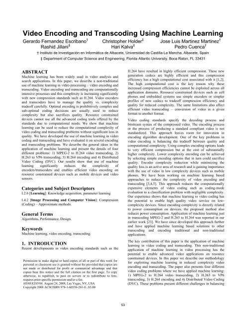
ABSTRACT 

Machine learning has been widely used in video analysis and 

search applications. In this paper, we describe a non-traditional 

use of machine learning in video processing – video encoding and 

transcoding. Video encoding and transcoding are computationally 

intensive processes and this complexity is increasing significantly 

with new compression standards such as H.264. Video encoders 

and transcoders have to manage the quality vs. complexity 

tradeoff carefully. Optimal encoding is prohibitively complex and 

sub-optimal coding decisions are usually used to reduce 

complexity but also sacrifices quality. Resource constrained 

devices cannot use all the advanced coding tools offered by the 

standards due to computational needs. We show that machine 

learning can be used to reduce the computational complexity of 

video coding and transcoding problems without significant loss in 

quality. We have developed the use of machine learning in video 

coding and transcoding and have evaluated it on several encoding 

and transcoding problems. We describe the general ideas in the 

application of machine learning and present the details of four 

different problems: 1) MPEG-2 to H.264 video transcoding, 2) 

H.263 to VP6 transcoding, 3) H.264 encoding and 4) Distributed 

Video Coding (DVC). Our results show that use of machine 

learning significantly reduces the complexity of 

encoders/transcoders and enables efficient video encoding on 

resource constrained devices such as mobile devices and video 

sensors. 

Categories and Subject Descriptors 

I.2.6 [Learning]: Knowledge acquisition, parameter learning 

I.4.2 [Image Processing and Computer Vision]: Compression 

(Coding) – Approximate methods. 

General Terms 

Algorithms, Performance, Design. 

Keywords 

Machine learning, video encoding, transcoding. 

1. INTRODUCTION 

Recent developments in video encoding standards such as the 

Permission to make digital or hard copies of all or part of this work for 

personal or classroom use is granted without fee provided that copies are 

not made or distributed for profit or commercial advantage and that 

copies bear this notice and the full citation on the first page. To copy 

otherwise, to republish, to post on servers or to redistribute to lists, 

requires prior specific permission and/or a fee. 

MDM/KDD'08, August 24, 2008, Las Vegas, NV, USA 

Copyright 2008 ACM ISBN 978-1-60558-261-0...$5.00 

Christopher Holder ‡ 

Hari Kalva ‡ 

Jose Luis Martinez Martinez † 

Pedro Cuenca † 

† Instituto de Investigación en Informática de Albacete, Universidad de Castilla-La Mancha, Albacete, Spain 

‡ Department of Computer Science and Engineering, Florida Atlantic University, Boca Raton, FL 33431 

53 

H.264 have resulted in highly efficient compression. These new 

generation codecs are highly efficient and this compression 

efficiency has a high computational cost associated with it [1,2]. 

The high computational cost is the key reason why these 

increased compression efficiencies cannot be exploited across all 

application domains. Resource constrained devices such as cell 

phones and embedded systems use simple encoders or simpler 

profiles of new codecs to tradeoff compression efficiency and 

quality for reduced complexity. The same limitations also affect 

efficient video transcoding – conversion of video in a given 

format to another format. 

Video coding standards specify the decoding process and 

bitstream syntax of the compressed video. The encoding process 

or the process of producing a standard compliant video is not 

standardized. This approach leaves room for innovation in 

encoding algorithm development. One of the key problems in 

video encoding is balancing the tradeoff between quality and 

computational complexity. Using complex encoding options leads 

to very efficient compression but at the cost of substantially 

higher complexity. Lower complexity encoding can be achieved 

by selecting simple encoding options that in turn could sacrifice 

quality. Encoder complexity reduction while minimizing the 

quality loss is an active area of research and is gaining importance 

with the use of video in low complexity devices such as mobile 

phones. We have been working on machine learning based 

approaches to reduce the complexity of video encoding and 

transcoding [3,4,5]. This approach reduces the computationally 

expensive elements of video coding such as coding-mode 

evaluation to a classification problem with negligible complexity. 

Our experience shows that machine learning to video coding has 

the potential to enable high quality video service on lowcomplexity 

devices. Since encoding complexity is directly related 

to power consumption on devices, the proposed method also 

reduces power consumption. Application of machine learning just 

in transcoding MPEG-2 and H.263 to H.264 was reported in our 

earlier work [23]. We have since developed this approach further 

and have applied machine learning based solutions to other 

transcoding and encoding traditional and non-traditional 

applications. 

The key contribution of this paper is the application of machine 

learning in video coding and transcoding. This non-traditional 

application of machine learning in video processing has the 

potential to enable advanced video applications on resource 

constrained devices. In this paper we describe our methodology 

for exploiting machine learning in reduced complexity video 

encoding and transcoding. The paper also presents four different 

video coding problems where we have applied machine learning: 

1) MPEG-2 to H.264 video transcoding, 2) H.263 to VP6 

transcoding, 3) H.264 encoding and 4) Distributed Video Coding 

(DVC). These problems present different challenges in balancing

the quality complexity tradeoff. The results show that machine 

learning techniques can reduce the complexity significantly with 

negligible loss in quality. 

2. MACHINE LEARNING AND VIDEO 

CODING 

Machine learning has been widely used in image and video 

processing for applications such as content based image and video 

retrieval (CBIR), content understanding, and video mining. The 

key to successfully employing machine learning for low 

complexity video coding is selection of attribute and the classifier 

to be able to reduce encoder coding mode selection to a 

classification problem. The attributes have to be computationally 

inexpensive and still be effective when used for classification. 

Since mode decisions are significantly influenced by the amount 

of detail and similarity among the macro blocks, features that 

describe the content can be used. MPEG-7 committee has 

standardized descriptors for describing content based features 

such as texture, color, shape, and motion [6]. Features such as 

homogenous texture could predict MB type and the edge 

histogram is potentially useful for deriving Intra MB prediction 

directions. While these features are potentially useful, the 

computational cost of extracting these features would offset any 

resulting complexity reduction. A feature set that uses negligible 

computation for feature extraction is necessary to develop low 

complexity video coding solutions. 

Our proposed approach is summarized in Figures 1. The basic 

idea is to determine encoder decisions such as MB coding mode 

decisions that are computationally expensive using easily 

computable features derived from input video. The input video is 

compressed in the case of transcoding problems and 

uncompressed in case of encoding problems. A machine learning 

algorithm/classifier is used to deduce the decision tree based on 

such features. Once a tree is trained, the encoder coding mode 

decisions that are normally done using cost-based models that 

evaluate all possible coding options are replaced with a decision 

tree. Decision trees are in effect if-else statements in software and 

require negligible computing resources. We believe this simple 

approach has the potential to significantly reduce encoding 

complexity and enable new class of video services. The key 

challenges in the proposed approach are: 1) Selecting the training 

set, 2) Determining the features/attributes, and 3) Selecting the 

classifier. 

(a) (b) 

Figure 1. (a) Applying machine learning to build decision 

trees (b) Low complexity video encoder using decision trees 

2.1 Selecting the Training Set 

Selecting a training set to encode all natural video is a challenging 

problem. The training set has to have all possible content for 

proper classification. On the other hand using a large training set 

could result in a large and complex decision tree. Upon closer 

54 

observation, the problem seems more manageable. Most of the 

video encoding mode decisions are based on the similarity 

(distance) of the block being encoded to those that are already 

coded. For Intra prediction in H.264, the similarity of the pixels in 

the current block to the edge pixels of the neighboring block 

determines the mode. For Inter MB coding, the similarity of the 

current block to the blocks in the previously coded frames 

determines the mode. A good training set should thus include not 

all possible colors and textures but enough blocks with similarity 

measures or distance metrics that are commonly found in typical 

video coding applications. Since video is usually encoded on a 

block-by-block basis, the training set should have enough blocks 

to ensure a good classification. The blocks selected for training 

can come from a single video or multiple video sequences. 

Considering that a frame of video at 720x480 resolution has 1350 

macro blocks, even a single frame of video can provide a 

sufficiently large training set. Such a training set is developed 

empirically. 

2.2 Determining the Video Features 

Image and video features have been used in content based 

retrieval of images and videos [7, 8]. The features that are 

typically used in content based retrieval describe the images and 

video segments. These features describe color, shape, texture, and 

motion and are developed for content retrieval and understanding 

applications. The features that are of interest in determining the 

coding modes are the similarity between current block and the 

previously coded blocks and the self-similarity of the current 

block. Simple metrics such as mean and variance could be 

sufficient to characterize a block coding mode. We have shown in 

our video transcoding work that variance of the DC coefficients 

of 8x8 blocks of an MPEG-2 Intra MB can be used to determine 

the Intra coding mode in H.264 [9]. Since the DC coefficient 

essentially gives the mean of a block, variance of means of 8x8 

sub-blocks could be used to characterize the Intra coding mode. 

However, as the number of coding modes increase, new features 

have to be developed to refine the classification of the coding 

modes. We have developed feature sets for each of the problems 

based on experimentation and performance analysis. We saw that 

the encoding complexity affects the resulting video quality. The 

use of more complex features improves the rate-distortion (RD) 

performance of an encoder but increase the computational 

complexity. The problems presented in Sections 3 to 6 discuss 

feature selection for the specific problems. 

2.3 Selecting the Classifier 

Classifier selection is another challenging task. The classifier has 

to be able to discover correlations between the attributes and 

classes. Classification algorithms have been used in content 

analysis in images and video [10,11]. These algorithms can be 

supervised or unsupervised. Since complexity reduction is the 

primary goal here, supervised learning is more appropriate. We 

use the general purpose classifier, C4.5 [12]. The C4.5 algorithm 

is shown to be a broad general purpose classifier that performs 

well for a large class of problems [13]. Our results showed that 

C4.5 performs very well for video coding problems. 

The decision tree for the transcoder was made using the WEKA 

data mining tool [14]. The files that are used for the WEKA data 

mining program are known as Attribute-Relation File Format 

(ARFF) files. An ARFF file is written in ASCII text and shows 

the relationship between a set of attributes. This file has two

different sections: 1) the header which contains the name of the 

relation, the attributes that are used, and their types; and 2) the 

section containing the data. The WEKA tool takes the ARFF file 

as input and outputs a decision tree and the corresponding 

confusion matrix. The decision trees are converted to a C++ code 

using a tree-to-C++ conversion tool we have developed and used 

in the encoder/transcoder implementation. 

2.4 Performance Evaluation 

The performance of video coding and transcoding is evaluated 

using an RD curve that shows a measure of distortion at a given 

bitrate. The RD curve alone shows coding efficiency and does not 

reflect complexity. Time complexity is measured as percentage 

reduction in video encoding or transcoding time compared to a 

reference method [18]. The goal is to achieve RD performance 

close to the reference methods at a significantly lower 

complexity. 

The performance of the decision tree (recall and precision) is 

important but not critical. In video coding applications, the cost of 

misclassification is reflected in reduced RD performance and the 

amount of performance loss is dependent on content and the type 

of misclassification. To reduce the impact of such 

misclassification, hierarchical decision trees are used such that a 

wrongly classified mode falls in a related mode. The learning 

stage is offline and supervised and the decision tree deduced is 

implemented in the encoder or transcoder. There is no way of 

determining the optimal mode at runtime and any feedback based 

refinement is not possible. The additional complexity due to this 

approach is implementation of feature computation and decision 

trees. With careful feature selection, this represents a negligible 

increase in complexity compared to the complexity reduced. 

Complexity is reduced because of the elimination of the cost 

based encoding mode selection. Since the mode selection no 

longer computes costs of all possible options, the modes used in 

machine learning based solutions are sub-optimal and lead to 

slightly reduced RD performance. 

3. MPEG-2 TO H.264 TRANSCODING 

The MPEG-2 video coding standard is widely used in digital 

video applications including digital TV, DVD, and HDTV 

applications. While MPEG-2 is widely deployed, a new video 

coding standard known as H.264 or MPEG-4 AVC is gaining 

significant interest due to its improved performance [1]. The 

H.264 video provides equivalent video quality at 1/3 to 1/2 of 

MPEG-2 bitrates. However, these gains come with a significant 

increase in encoding and decoding complexity [15]. Given the 

wide deployment of MPEG-2 infrastructure, MPEG-2 and H.264 

are likely to coexist even as H.264 systems are deployed. The 

coexistence of these technologies necessitates systems that can 

leverage MPEG-2 and H.264 to provide innovative digital video 

services making use of MPEG-2 for current devices and H.264 for 

new generation receivers. The key to making this seamless is by 

transcoding MPEG-2 to H.264 at the appropriate points in the 

video distribution infrastructure: at the sender, in the network, or 

even at the receiver. However, given the significant differences 

between both encoding algorithms, the transcoding process of 

such systems is a much more complex task than other 

heterogeneous video transcoding processes [16,17]. 

55 


The training sets were made using MPEG-2 sequences encoded at 

higher than the typical broadcast encoding rates for the same 

quality, since the B frames are not used. The H.264 decisions in 

the training set were obtained from encoding the MPEG-2 

decoded sequence with a quantization parameter of 25 and RD 

optimized mode decision option enabled. After extensive 

experimentation, we found that sequences that contain regions 

varying from homogenous to high-detail serve as good training 

sets. Good sample sequences could be Flower Garden and 

Football (sequences commonly used in video coding research). 

The goal is to develop a single, generalized, decision tree that can 

be used for transcoding any MPEG-2 video. We found that 

training based just on the Flower Garden sequence was sufficient 

to make accurate decisions for all videos, due to the complexity 

and variety of motion and texture in the sequence. 

The incoming video sequence, which is used to train the model, is 

decoded and during the decoding stage, the MB coding mode, the 

Coded Block Pattern (CBPC), and the mean and variance of the 

residual information for this MB (calculated for its 4x4 subblocks 

– resulting in 16 means and 16 variances for each MB) are 

saved. The decoded sequence is then encoded using the standard 

H.264 encoder. The coding mode of the corresponding MBs in 

H.264 is also saved. For each macroblock, each of one of the 

instances in the training set uses the following predictive 

attributes: i) Thirty two numerical variables: sixteen means and 

sixteen variances of the 4x4 motion estimation residual subblocks, 

ii) the MB mode in MPEG-2, iii) the CBPC in MPEG-2, 

iv) and the corresponding H.264 MB coding mode decision for 

that MB as determined by the standard reference software. 

Finally, the class variable, i.e, the one that we are trying to 

understand, classify, or generalize is the H.264 MB coding mode, 

and can take four values: skip, 16x16, 8x8 or Intra, in the first 

level of the decision tree proposed. 

3.2 Decision Trees 

The decision tree, that we are going to proposed to solve the interprediction 

problem, is a model of the data that encodes the 

distribution of the class label (MB mode in H.264) in terms of the 

attributes (MB mode in the incoming sequence, CBPC, Mean and 

Variance), as we resumed in the previous sub-section. Figure 2 

shows the decision trees built 

using the process depicted in 

Figure 1. 

As shown in Figure 2, the 

Decision Tree for the proposed 

transcoder is a hierarchical 

decision tree with three different 

WEKA trees: 1) classifier for 

Figure 2. The Decision Tree 

Intra, Skip, Inter 16x16, and 

Inter 8x8, 2) classifier to classify inter 16x16 into one of 16x16, 

16x8, and 8x16 MBs and 3) classifier to classify inter 8x8 into 

one of 8x8, 8x4, 4x8, or 4x4. 

Flower garden sequence produces datasets with 1204, 906, and 

256 instances; and 38, 38 and 14 attributes used to train the 

decision trees placed in node1, node3 and node4 respectively. 

Table 1 summarizes the decision trees obtained from the learning 

process; #leaves, #nodes and #vars stand for the number of leaves,

inner nodes and variables included in the tree. These statistics can 

give us a measure about the complexity of the learnt trees, 

because the number of leaves coincides with the number of 

generated rules and the number of nodes gives us an idea about 

the number of conditions to be tested per rule. 

Table 1. Main data for the trees 

MPEG-2 to H.264 

#leaves #nodes #vars e(10CV) 

Tree at Node1 27 23 17 15.11 

Tree at Node3 63 59 32 28.80 

Tree at Node4 13 9 7 28.20 

As we can see the number of rules is not excessive, 103 for the 

MPEG-2 hierarchical classifier, and from the number of inner 

nodes we observe that the obtained rules have few conditions to 

be tested in their antecedent. With respect to the number of 

variables used in the tree, it is clear that it is in the first level when 

more variables can be considered as redundant because only 17 

are used from the 38 available. With respect to the last column, it 

shows the expected error for our classifier computed by using a 

standard technique as it is 10 fold cross-validation (10cv). 

Table 2 shows the error obtained when using a classifier learnt 

using the training set obtained from the Flower Garden sequence, 

and using as test set the arff files obtained from three different 

sequences: Akiyo, Paris and Tempete (n/a means that the result is 

not available because no records where labeled as 8x8 in the 

Akiyo sequence). The goal of this experiment is to show the 

generalization power of the learnt classifiers, i.e., its capability 

when used to test unseen sequences. As we can see the average 

error in each level is even lower than the cross validated error 

computed over the Flower Garden sequence (the sequence used 

for training), so we can conclude that our classifiers exhibit a 

good generalization behavior. 

Table 2. Results of evaluating the learnt classifier 

MPEG-2 to H.264 

Akiyo Paris Tempete 

Tree at Node1 13.40 12.28 14.06 

Tree at Node3 0.00 23.30 42.14 

Tree at Node4 n/a 18.75 8.33 


In order to evaluate the proposed macroblock partition mode 

decision algorithm for heterogeneous MPEG-2 to H.264 video 

transcoder proposed in this section, we have implemented the 

proposed approach based on the JM10.2 version of the H.264 

reference software. The additional computation here is the 

computation of the mean and variance of the 4x4 sub-blocks of 

the residual MBs. The MB coding mode decision determined by 

the decision trees is used in the low complexity H.264 encoding 

stage. This is an H.264 reference encoder with the MB mode 

decision replaced by simple mode assignment from the decision 

tree. The H.264 video encoder takes as input the decoder MPEG- 

2 (pixel data), the residual information, the mode decision and the 

CBPC for each macroblock of the P frames. 

Experiments were conducted to evaluate the performance of the 

proposed algorithm when transcoding videos at CIF resolution. 

The input bit-rate for the MPEG-2 sequences is 1.15 Mbits/sec 

(progressive format), the GOP size is 12 -I11(P)-, and the 

maximum motion search range is 15. 

56 

For re-encoding the input sequences, we use quantization 

parameters (QP) from QP = 28 to QP = 40. The size of the GOP is 

12 frames; with the same GOP format than in the input sequences. 

The rate control and CABAC algorithms were disabled for all the 

simulations. RD-optimized option is enabled. The number of 

reference in P frames was set to 1 and the motion search range 

was set to ± 16 pels with a MV resolution of ¼ pel. The 

ProfileIDC was set to High for all the simulations, with the FRExt 

options enabled. The other parameters were set to the default 

option. The time results were normalized, so they are independent 

from the machine used to run the simulations. The results are 

reported for five different sequences. The performance of the 

proposed very low complexity transcoder is compared with a 

reference transcoder comprised of a full MPEG-2 decoder 

followed by a full H.264 encoder. The metrics used to evaluate 

the comparative performance are: the rate-distortion function, the 

difference of coding time (∆Time), the PSNR difference (∆PSNR) 

and the bit-rate difference (∆Bitrate). The detail procedures in 

calculating these differences can be found from a JVT document 

authored by Bjontegaard [18]. 

Akiyo 

Paris 

Stefan 

Tempete 

Figure 3. Rate Distortion Results 

Figure 3 shows the Rate Distortion results of applying the 

following options: Full RD-optimized H.264 encoding with the 

reference transcoder and the proposed low complexity H.264 

encoding stage, in the MPEG-2/H.264 transcoder scenario. The 

PSNR obtained when applying our algorithm deviates slightly 

from the results obtained when applying the considerably more 

complex full RD-optimized H.264 encoding with the MPEG- 

2/H.264 reference transcoder. 

Mobile 

Table 3. ΔBitRate, ΔPSNR and Time Reduction results. 

Proposed (MPEG-2/H.264) 

Sequence Time (%) ΔPSNR (dB) ΔBitRate (%) 

Akiyo - 72.49 - 0.052 1.78 

Paris - 73.63 - 0.083 3.75 

Tempete - 71.01 - 0.045 2.95 

Stefan - 71.10 - 0.245 13.76 

Mobile - 70.04 - 0.012 0.96 

Table 3 shows the results in terms of ∆Time, ∆PSNR and ∆Bitrate 

for the proposed data mining based encoding stage compared with 

the RD optimized encoding stage for encoding 200 frames of each 

sequence. PSNR and bit-rate differences are calculated according

to the numerical averages between 

the RD-curves derived from JM 

encoder, the algorithm under study. 

The negligible drop in RD 

performance is more than offset by 

the reduction in computational 

complexity. However, in terms of 

time saving, which is a critical issue 

in video transcoding applications, 

Table 5: MB mode distribution in VP-6 

Inter 0,0 Intra 

the proposed method significantly reduces the time for reencoding 

the sequences. 

4. FLASH VIDEO TRANSCODING 

Adobe’s Flash video has become the dominant format for video 

distribution on the Internet. Flash 6 video format is essentially 

H.263 and a lot of content exists in this format. Flash 8 used VP6 

compression for video. Flash 8 is widely used today even as Flash 

9 with additional H.264 support became available. Flash video 

transcoding transcodes H.263 to VP-6 formats to enable low 

complexity Flash 6 to Flash 8 transcoding. 

H.263 is a video coding standard developed under the auspice of 

the ITU. The standard was developed targeting low bitrate video 

applications in telecommunications. H.263 is a hybrid video 

coding format similar to the MPEG video codecs. The baseline 

profile of H.263 with Annex-D, unrestricted motion vector mode, 

and Annex-F, Advanced prediction mode, is used as the input to 

the transcoder. 

Table 4: Comparison of VP6 and H.263 Coding Features 

Feature H.263 Baseline VP6 

Picture type I, P I, P 

Transform size 8x8 8x8 

Transform DCT Integer DCT 

Intra prediction None None 

Motion comp. 16x16, 8x8 16x16, 8x8 

Total MB modes 4 10 

Motion vectors ½ pixel ¼ pixel 

Deblocking filter None Yes 

Reference frames 1 Max 2 

VP6 is a proprietary video compression algorithm developed by 

On2 Technologies. VP6 is also a hybrid codec that uses motion 

compensated transform coding at its core. Motion compensation 

supports 16x16 and 8x8 blocks similar to H.263 but the Inter 8x8 

macro blocks can have mixed blocks; i.e., one or more 8x8 blocks 

can be coded in Intra mode without using any prediction. The 

Inter MBs in VP6 can be coded using 9 different modes. The 

modes are characterized by the number of motion vectors (1 vs. 

4), reference frame used, and whether motion vectors are coded. 

Table 4 summarizes the similarities and differences between 

H.263 baseline profile and the VP6 encoder. The large number of 

coding modes supported in VP6, the ¼ pixel resolution motion 

vectors, and multiple reference frames allowed make transcoding 

from H.263 to VP6 difficult. The transcoding algorithms are 

designed for Inter frames and focus on reusing the motion 

information. 


Training set selection was important for this transcoder. Both of 

the video standards used in the Flash transcoder have much lower 

complexity compared to H.264. This gives the challenge of 

Inter+ 

MV 

Nearest Near Golden Golden 

MV 

Inter 

4V 

Golden 

Nearest 

providing low complexity calculations for the attributes used for 

these trees. The variables which are used are based off the residue 

from the macroblock for the decoded frame. Since the smallest 

block size available in VP6 is 8x8, the means of the 4x4 blocks 

were not used. Also only the residue of the luma was used for the 

means. The means of 8x8 and 16x16, variance of the 16x16, the 

coded block pattern and also the inter 0,0 error (difference with 

collocated block in reference frame) was used. The coded block 

pattern is the binary representation of the coded blocks in a macro 

block. Because of VP6 implementation, the inter 0,0 decision has 

to be generated for all decisions so using it into the tree does not 

add complexity. The variables chosen have low complexity and 

are calculated using integer arithmetic to avoid floating point 

complexity. 

The training process was performed by using eight different 

sequences. The first P frame of each was use for the data to 

produce the trees. Also all combinations of the attributes were 

evaluated in order to determine the attributes that result in best 

classification. These trees were then tested against a test file 

which contained 100 frames of each of the training sequences. 

The best tree was chosen for its accuracy and confusion matrix 

which had the best precision. 


Table 5 shows how each of the H.263 MBs are coded in VP6 for a 

typical sequence. Based on Table 5, one can observe that the 

distribution of the modes greatly depends on the H.263 mode. 

With C4.5, the modes which are in the minority have a good 

chance of being misclassified and overlooked. However, having 

separate trees which depend on the H.263 mode allows proper 

classification of minority modes. This results in much more 

efficient decision trees. This multi-tree approach also reduces 

misclassification on the Inter 4V and Intra modes. 

Figure 4. Decision trees used in VP-6 transcoding (a) 

Flawed top (b) H.263 Mode Separated trees 

Golden 

Near 

Inter 17% 0% 21% 38% 21% 0% 1% 2% 0% 0% 

Inter 4V 3% 1% 30% 11% 7% 1% 1% 47% 0% 0% 

Intra 11% 33% 4% 9% 4% 11% 3% 19% 4% 2% 

Skipped 60% 0% 0% 31% 8% 0% 0% 0% 0% 0% 

57 

Our experiments showed that hierarchical trees preformed better 

than a tree which had only one level and many decisions. Figure 4 

shows two of the multi-level trees used. The goal is to classify the 

MB coding mode into one of Skip, Inter 1MV, or Inter 4 MV. 

Classifying H.263 MB into three classes is error prone and a 

hierarchical classifier was designed. Different configurations of 

trees were evaluated, but not all will be discussed because of 

space considerations. The two trees with the best results were : 1) 

H.263 Mode Separated trees 2) Flawed Top tree. These are shown 

in Figure 4.

The H.263 Mode Separated tree (Fig. 4.b) had four trees for each 

of the H.263 modes and each of these trees selects one of three 

VP-6 modes. This has low complexity and the ability to predict 

accurately. The Flawed Top tree is a hierarchical tree with the top 

level tree making skipped vs. non-skipped decision. Because of 

implementation dependencies, Intra cost is evaluated before any 

of the tree decisions are invoked. Some MBs may be coded as 

Intra if the Intra cost evaluated is lower than the cost of mode 

selected by the trees. Four second level trees (2 – 5 in Fig. 4.a), 

for each of the four H.263 modes, are trained with data which 

would have come from first tree. This tree classifies the MB into 

one of the two modes. 


All the results reported in this paper use the TMN 3.2 H.263 

encoder from University of British Columbia which is based on 

Telenor's H.263 implementation. The input video is coded at 512 

Kbps in baseline profile with advanced motion options and one I 

frame (first frame). A decoder based on the same H.263 

implementation is used in the decoding stage of the transcoder. 

The VP-6 encoding stage is based on the optimized VP-6 encoder 

software provided by ON2 Technologies. The VP-6 video is 

encoded with I frame frequency of 120 and at multiple bitrates to 

assess the RD performance of the transcoder. The results are 

compared with the baseline transcoder that performs full encoding 

in the VP-6 encoding stage. 

Table 6. The RD performance of the Trees 

Decision tree/Sequence used 

PSNR (dB) 

35 

34 

33 

32 

31 

30 

29 

28 

Time 

(%) 

Rate vs. Distortion (352x288, CIF) 

ΔPSNR 

(dB) 

CoastGuard Baseline 

CoastGuard H.263 Seperated 

CoastGuard Flawed Top 

Football Baseline 

Football H.263 Seperated 

Football Flawed Top 

27 

0 200000 400000 600000 

Bitrate 

800000 1e+006 

Figure 5. Transcoder performance 

ΔBitrate 

(%) 

H.263 separate trees/Coastguard -48.4 0.10 2.09 

H.263 separate trees/Football -50.7 0.12 6.15 

Flawed top/Coastguard -39.0 0.10 2.74 

Flawed top/Football -44.1 -0.12 -1.75 

The RD performance of the transcoder using the full set of trees 

evaluated is shown in Table 6. The results show that the RD 

performance is very close to the baseline transcoder. Figure 5 

shows the average transcoder performance summary for two of 

the tested sequences transcoded from 128 Kbps to 512 Kbps. The 

H.263 mode separated tree gives the best performance as this 

minimizes the additional computation for mode decision. This 

tree uses a single decision tree for each MB based on the H.263 

mode while the Flawed Top tree uses two decision trees. The 

58 

results show that the speedup can be as high as 2.1. The average 

speedup is 1.7; i.e., transcoding algorithms increase the transcoder 

capacity by 70%. Considering that the VP-6 encoder is an 

optimized implementation, 70% improvement is a highly 

significant improvement. 

5. H.264 ENCODING 

In this section we present the application of machine learning in 

Intra frame encoding in H.264. H.264/AVC is the state of the art 

video compression standard and has been designed for a wide 

range of applications. The compression efficiency of H.264 has 

increased mainly because of the large number of coding options 

available. For example, the H.264 video supports Intra prediction 

with 3 different block sizes (plus up to 9 prediction directions per 

block size) and Inter prediction with 8 different block sizes. The 

encoding of a macro block (MB) is a complex operation as it 

involves evaluating all the possible coding options and selecting 

an option that has the least cost associated with it. Most H.264 

encoder implementations on mobile devices today do not 

implement the standard profiles fully due to high complexity. 

The key idea behind this approach is to exploit the correlation 

between the structural information in a video frame and the 

corresponding H.264 MB mode decisions. In this approach, 

encoder decisions such as MB coding mode decisions that are 

computationally expensive are replaced with mode decisions from 

a low complexity decision tree (see Fig. 1). 


The training set of videos was selected based on the extensive 

empirical experiments. The results from one sequence were 

verified by cross validating with the other sequences. Based on 

our observations from our earlier work (MPEG-2 to H.264 

encoding and DVC encoding), Flower Garden and Mobile are the 

best training sequences as discussed in the relevant sections of 

this paper. To generate a single generic decision tree which 

produces optimal results for all sequences is very difficult; 

therefore, a best compromise is chosen to apply to all sequences 

to minimize the drop in RD performance. 

Training set of a sequence that is used as an input to WEKA 

contains the attribute values and the MB mode selected for each 

MB. The number of instances used to get good decision trees vary 

for 16x16 and 4x4 modes. Since the number of 4x4 modes can be 

greater than that of 16x16 modes in a given frame, therefore we 

need more frames to create training set for 16x16 modes and less 

frames to create training set for 4x4 modes. For each macroblock, 

the training set for top level node decision (Intra 16x16 vs. Intra 

4x4) involves only two attributes i.e. mean of MB and variance of 

16 4x4 means in an MB and also the corresponding H.264/AVC 

MB coding mode decision for that MB as determined by the 

standard reference software. The number of attributes is carefully 

determined based on the observations about the properties of the 

attributes chosen and the resulting performance. For example, 

deciding between Intra 16x16 and Intra 4x4 modes largely 

depends upon the homogeneity within the macroblocks, therefore, 

mean of MB and variance of means of 16 4x4 blocks of an MB 

are very helpful for the decision at this level. For lower level 

nodes of the decision tree, more complex attributes were 

calculated and used such as right/left columns and top/bottom 

rows of an MB.

Training set was generated by using the 8 CIF frames of the 

Flower Garden sequence by using the I frames only. QP was 

selected at 28 and Rate Distortion (RD) optimized mode decision 

option disabled. QP was scaled according to the applied QP value 

while using the decision trees at the later stage. As for the 

attributes extracted from each MB (8 CIF frames x 396 blocks per 

frame, a total of 3168 instances were included in the training set), 

the following measures were taken into account: mean, variance, 

the variance of the means, and different measures of right/left 

columns and top/bottom rows. For each macroblock in Intra 

16x16 decisions, each of one of the instances in the training set 

uses the combination of following different predictive attributes: 

i) sixteen means and sixteen variances of the 4x4 blocks of an MB 

of a frame data, ii) the variances of top/bottom rows and right/left 

columns of an MB, iii) the difference of means of the bottom row 

of top MB and bottom row of current MB, iv) the difference of 

means of the right column of left MB and right column of current 

MB, v) and the corresponding H.264 MB coding mode decision 

for that MB as determined by the standard reference software. 

The training set for the Intra 4x4 modes involves more complex 

attributes obtained from 4x4 blocks in an MB by experimenting 

with different combinations of these attributes. Due to the space 

constraint, we cannot explain the formation of the attributes for 

Intra 4x4 decisions. 


Intra MBs in H.264 are coded as Intra 16x16, Intra 4x4, or Intra 

8x8. The baseline profile used in mobile devices does not support 

Intra 8x8 mode and this mode will not be discussed further in this 

paper. Intra modes also have associated prediction modes; Intra 

16x16 has 4 prediction modes and Intra 4x4 has 9 prediction 

modes. Baseline profile encoders typically evaluate both Intra 

16x16 and Intra 4x4 modes and the associated prediction modes 

before making MB mode decisions. In the proposed machine 

learning based approach we separate the Intra MB mode and Intra 

prediction mode decisions. Intra MB mode is determined as Intra 

16x16 or Intra 4x4 without evaluating any prediction modes. The 

appropriate prediction modes for the MB mode are then 

determined. Since the MB mode is determined first, our approach 

right away eliminates the computation of any prediction modes 

for the MB mode that is not selected. If the MB mode is 

determined to be Intra 16x16, there is no need to evaluate any 

prediction modes for the 4x4 sub-blocks. 

Our proposed decision tree divides the Intra decision into two 

categories at the top most level i.e. Intra 16x16 and Intra 4x4 as 

shown in Figure 6. The sub-tree on the left calculates the Intra 

16x16 decisions while sub-tree on the right calculates the Intra 

4x4 decisions. This figure also shows that we have four different 

WEKA trees to classify all of the 16x16 mode decisions while all 

4x4 modes decisions are classified in nine WEKA trees. Flower 

garden sequence used to create decision trees contains a datasets 

with 3168, 1384, 950 and 434 instances for nodes 0, 1, 3 and 4 

respectively. Table 7 shows the characteristics of the classifiers 

obtained for Intra 16x16 encoding. CCI stands for correctly 

classified instances and is computed by using a standard 

technique called cross-validation while rest of the columns is the 

same as explained in Section 3.2. 

The total number of rules for determining all Intra 16x16 modes is 

35. The emphasis of our experiments was to keep the number of 

59 

variables (attributes) minimum and the size of the tree as short as 

possible. Table 8 shows the CCI percentage for different 

sequences when decision tree obtained by using one sequence at 

one node is applied to the remaining sequences. 

Figure 6. The Decision Tree 

Table 7. Decision Tree Statistics for Intra 16x16 Nodes 

Fast H.264/AVC Encoding 

#leaves #nodes #vars CCI (%) 

Node 0 4 7 2 97.92 

Node 1 14 27 7 76.66 

Node 3 7 13 4 76 

Node 4 10 19 7 76.96 

Table 8. CCI % of the learnt classifiers 

Fast H.264/AVC Encoding 

Akiyo Coastguard Container Mobile 

Node 0 78 92 86.69 98.65 

Node 1 62.95 66.96 65.28 63.70 

Node 3 66.21 63.63 65.90 62.39 

Node 4 65 60 62 72.68 


The proposed decision trees obtained from training sequences 

were implemented in the H.264/AVC reference software JM 13.2. 

Attributes calculation (used in decision trees) takes up additional 

computation time but our algorithm bypasses the standard H.264 

mode detection algorithm which in turn saves the considerable 

encoding time. 

Experiments were conducted to evaluate the performance of the 

proposed algorithm by encoding sequences at CIF and QCIF 

resolution by enabling the I frames only. RD optimization was 

disabled and also no rate control mechanism was employed while 

performing these experiments. To analyze the performance of our 

approach, encoder parameters were kept consistent and 

unchanged during both stages, i.e. training and encoding, so that 

the RD performance could be measured without any bias. 

Figure 7 shows the RD performance results of applying the 

decision trees. Figures 7.a, 7.c are CIF resolution of Coastguard 

and Foreman sequences while Figures 7.b, 7.d are QCIF 

resolution of the same sequences. We implemented the decision 

tree in order to evaluate the performance of the machine learning 

based decisions. The Intra MB decisions in JM13.2 were replaced 

by a decision tree, a set of if-else statements. Performance is 

evaluated by comparing the RD performance of an encoder with 

the proposed methods for Intra mode decisions and a standard 

encoder. The results show that Intra 16x16 MB mode decisions 

can be made with very high accuracy; as shown in Figure 7.(a-d). 

Prediction mode decisions are complex and introduce a small loss 

in PSNR. The average PSNR loss suffered in all sequences is

about 0.03 dB while the average bitrate increase is 8%. The 

encoding time of the proposed method is about 1/3 of the 

reference encoding time. 

PSNR (dB) 

PSNR (dB) 

45 

40 

35 

30 

25 

45 

40 

35 

30 

Rate vs. Distortion (Coastguard, 352x288, CIF) 

Baseline 

Proposed 

0 1000 2000 3000 4000 5000 6000 7000 8000 

Bitrate (Kb/s) 

25 

0 1000 2000 3000 4000 5000 6000 7000 


PSNR (dB) 

45 

40 

35 

30 

25 

Rate vs. Distortion (Coastguard, 176x144, QCIF) 

Baseline 

Proposed 

0 500 1000 1500 2000 2500 


a) b) 

Rate vs. Distortion (Foreman, 352x288, CIF) 

Baseline 

Proposed 

PSNR (dB) 

45 

40 

35 

30 

Rate vs. Distortion (Foreman, 176x144, QCIF) 

Baseline 

Proposed 

25 

0 500 1000 1500 2000 2500 


c) d) 

Figure 7. Rate Distortion Results 

Table 9 shows the results in terms of ∆Time, ∆PSNR and ∆Bitrate 

for the proposed data mining based encoding approach compared 

with the baseline encoder. The drop in RD performance is 

compensated by the reduction in computational complexity. 

However, in terms of time saving, which is a critical issue in 

video transcoding applications, the proposed method significantly 

reduces the time for encoding the sequences. 

Table 9. ΔBitRate, ΔPSNR and Time Reduction results 

Proposed (Intra H.264/AVC encoding) 

Sequence Time (%) ΔPSNR (dB) ΔBitRate (%) 

Akiyo - 26.54 - 0.012 9.45 

Coastguard - 17.21 -0.032 8.57 

Container - 15.46 - 0.072 9.38 

Stefan - 21.67 - 0.021 6.75 

Mobile - 33.71 - 0.017 4.87 

6. DVC ENCODING 

DVC is a technique used to reduce the asymmetry in video 

codecs; the processing complexity of the encoders is reduced, 

leading to a low-cost implementation and the complexity of the 

decoders is increased. This architecture is desirable for 

applications where the cost, complexity and power consumptions 

features of the encoder are very critical. The theoretical 

framework of DVC was developed by Slepian-Wolf (SW) [19] for 

lossless Distributed Source Coding (DSC) and by Wyner-Ziv 

(WZ) [20] for the lossy case. This mathematical background 

states that, under the same conditions, the RD performance 

achieved in traditional video coding scheme [1] can also be 

obtained by DVC [21] scheme. 

A good introduction to DVC is provided in [21]. To summarize, 

DVC scheme is based on the idea of determining an 

approximation at the decoder side of the current frame which is 

available at the encoder. This estimation is commonly labeled as 

side information. A DVC decoder’s task is to correct the possible 

mismatches between this side information and the original frame 

60 

using parity bits sent by the encoder that have been generated 

from the current frame. Most of the architectures discussed in the 

literature are based on [21] and make use of a feedback or reverse 

channel to the encoder to request parity bits. Furthermore, the 

mismatches are determined in these theoretical models by 

assuming ideal error estimation that relies on the availability of 

the original frame at the decoder. The process of requesting and 

receiving the parity bits from the encoder in order to reduce the 

mismatches is referred to as rate control in DVC. 

This feedback based architecture with ideal error estimation 

assumption creates significant problems in developing practical 

DVC encoders: original frames are not available at the decoders 

and bidirectional communication channels may not be always 

available. New approaches are necessary to solve both if these 

problems while keeping the low complexity encoder devices 

promised by DVC. Machine learning based techniques can 

potentially enable an efficient and very low complexity rate 

control algorithm used in DVC systems. Machine Learning is 

likely to be useful because there exits a correlation between some 

information available at the encoder and the number of parity bits 

or number of requests over this feedback channel. 

(a) Current frame 

(b)Faster average side information at 

the encoder 

(d) Residual frame. 

ZERO REQUEST 

MINIMUN REQUEST 

MEDIUM REQUEST 

MAXIMUN REQUEST 

(c) Best MCTI side information 

generated at the decoder 

(e) N# requests of the first frame. 

Figure 8. Exploiting the correlation using Machine Learning 

Figure 8.c is the estimate computed at the decoder of the current 

frame available at the encoder (Fig. 8.a). This side information 

has been computed using more sophisticated Motion 

Compensated Temporal Interpolation (MCTI) tool that represents 

one of the more complex tasks performed at the decoder. In low 

complexity DVC encoders, the MCTI operation is unviable 

because of complexity considerations. Therefore, a simple 

estimate of the side information, the average between 

past/previous key frames is used (Figure 8.b). The problem then is 

correcting the residual frame (the difference between original and 

side information) information using these parity bits. Figure 8.d 

and 8.e show the motivation behind the use of ML to try to 

determine the number of requests. The Figure clearly shows that

there exits a correlation between the amount of information 

available in the residual frame and the number of requests (parity 

bits). If an encoder can estimate the number of requests a decoder 

would make to reach a given quality, then the encoder can send 

those parity bits even without requests from the decoder and 

thereby eliminating the need for the feedback channel. It is clear 

from these figures that the residual information is higher for the 

blocks where the number of requests (bits requests) is also higher 

and vice versa. 


The training sets were made using sequences that have gone 

through the procedure to get the residual image (See Figure 8.d) 

and then we have extracted some solid information about each 

residual frame. The number of requests were extracted from these 

same sequences over a feedback based architecture [24] working 

at block by block level. After extensive experimentation, we 

found that sequences that contain regions varying from 

homogenous to high-detail serve as good training sets. Moreover, 

sequences which show all kind of textures and features movement 

can be enough. Good sample sequences could be Flower Garden 

and Mobile. The number of instances in a proper training set has 

to be selected carefully as we are trying to develop a single, 

generalized, decision tree. Using too many instances can over 

adjust the results for this sequence (the training sequence) and can 

not be a generic tree. 

Finally, the training set was generated using five QCIF frames of 

the Flower Garden sequence. As for the attributes extracted from 

each 4x4 (5 QCIF frames x 1584 blocks per frame, a total of 7920 

instances) block of the residual frame, the following measures 

were taken into account: mean, variance, the variance of the 

means. In our study, we showed that the variance of the 2x2 subblock 

means (the variance of means attribute) is a good estimator 

of the amount intensity available in the 

residual frame. The pixel domain DVC 

architecture process bitplane by bitplane; 

that is, the pixel values are quantized using 

a 2 M – level uniform quantizer; in this case 

2 M ∈ {2, 4, 8}, different training sets 

were created depending on which bitplane 

is processed and, therefore, the statistical 

information was extracted from this m ≤ 

2 M bitplanes. The decision tree for the rate 

encoder control was made using the 

WEKA data mining tool. 

Figure 9. Rate 

Encoder Decision Tree 


The decision tree consists of three WEKA decision trees, shown 

in Figure 9 with numbered circles. In our previous works [22] we 

implemented a non-binary tree and we showed some deficiencies 

and this results were improved using a binary tree as shown in 

Figure 9. The order of decision has an important impact on the 

overall performance. We found that best performance is achieved 

when the easiest decision is taken at the first decision level and 

leaving the more complex decisions for the bottom levels. 

Looking at our rate allocation problem and the Figure 8.d and 8.e, 

the decision whether a block needs some parity or not is the 

easiest and corresponds to the non information residual areas in 

Figure 8.d collocated with ZERO-REQUEST labeled blocks. 

61 

Therefore the first level decision tree split the decision into 

ZERO-REQUEST and NON-ZERO-REQUEST. The following 

decision trees (second and third level) try to continue classifying 

into the different REQUEST labels. For the NON-ZERO- 

REQUEST tree, the tree takes the different label block decision 

based on the energy available in the residual frame. The second 

level decision checks between the MAX-REQUEST label and the 

rest of possibilities following the same principle used in the first 

level decision: it is easiest to determine if a block will spend the 

maximum rate (a poorly estimated block in the side information 

frame) or not. Finally, in the last level, the decision is made over 

MIN-REQUEST or MED-REQUEST. Each node decision of the 

tree takes the decision based on predefined threshold of the 

statistical information extract form the residual frame. Table 10 

shows the characteristics of the classifiers obtained for feedback 

free DVC codec for the first bitplane processing (the lowest 

bitrate point). 

Table 10. Decision Tree Statistics 

Rate Allocation at the encoder 

#leaves #nodes #vars e(10CV) 

Tree at Node1 7 13 3 17.58 

Tree at Node2 2 3 1 16.10 

Tree at Node3 2 3 1 11.36 


The RD performance evaluation of our scheme is shown in Figure 

10 for sequences commonly used in the literature. As we can see, 

the RD performance is negligible for lower bitrates and increase a 

little for higher bitrates. At higher bitrates, more bit planes are 

processed (and more pixel details) and there are more differences 

between the side information generated at the encoder using low 

complexity algorithms compared to the more complex MCTI 

done at the decoder. The performance is very close to the 

theoretical Feedback Based solutions with optimal RD 

performance. The results also show a significant decoding 

complexity reduction of over 80%, and a negligible increase in 

encoder complexity; a maximum of 25% (for higher rates) 

increase compared to the impractical feedback based 

architectures. 

Table 11 Percentage of good choice per levels 

Tree at Container Foreman Hall Mother 

Node1 99.99 97.11 99.99 99.99 

Node2 81.18 71.06 78.27 80.07 

Node3 65.77 64.04 69.68 65.44 

Finally, Table 11 analyzes the accuracy of the data mining 

process discussed in this section in terms of % of good choice; i.e. 

the percentage of correctly labeled blocks compared to the 

feedback channel decision. As Table 11 shows the decision 

between ZERO REQUEST (Node 1 in Figure 10) and NON- 

ZERO REQUEST (Node 2 and Node 3 in Figure 10) are quasi 

optimal; 99 % on average. The nodes 2 and 3 that classify the 

NON-ZERO REQUEST (MAX, MED and MIN REQUEST) have 

a lower performance; 77 % and 66% on average, respectively. 

Therefore, the proposed feedback free architecture using machine 

learning brings DVC closer to a practical solution.

7. CONCLUSION 

This paper described the use of machine learning for video 

encoding and transcoding. We show that this non-traditional use 

of machine learning in video processing is highly effective in 

reducing the computational complexity. The role of machine 

learning in these applications is to predict a coding mode based on 

easily computable features and thereby avoiding the large amount 

of computation necessary for coding mode selection. We have 

implemented this approach in video transcoding, video encoding, 

and distributed video coding. We described the use of the 

proposed approach in four video coding applications. The results 

show that this approach works well across applications – gives 

significant complexity reduction with negligible drop in quality. 

With increasing complexity of video coding standards such as 

H.264, complexity reduction is critical to exploit all advanced 

coding features in resource constrained devices. We show that the 

proposed approach is general enough and can be used effectively 

in high complexity video coding and transcoding applications. 

Mother 

C ontainer 

Hall 

Fore m an 

Figure 10. RD Performance of low comlexity DVC 

8. ACKNOWLEDGMENTS 

This work was supported in part by On2 Technologies, Florida 

Atlantic University Research Corporation, the Spanish MEC and 

European Commission FEDER funds under grants “Consolider 

Ingenio-2010 CSD2006-00046”' and “TIN2006-15516-C04-02”', 

and by JCCM funds under grant “PAI06-0106”. 

9. REFERENCES 

[1] H. Kalva, “The H.264/AVC Video Coding Standard,” 

IEEE Multimedia, Vol. 13, No 4, Oct. 2006, pp. 86-90. 

[2] H. Kalva and J.B. Lee, “The VC-1 Video Coding 

Standard,” IEEE Multimedia, Vol. 14, No 4, Oct.-Dec. 

2007, pp. 88-91. 

[3] G. Fernandez-Escribano et. al., “A Fast MB Mode 

Decision Algorithm for MPEG-2 to H.264 P-Frame 

Transcoding,” IEEE Tran. on Cir. and Sys. for Video 

Tech., Feb. 2008, pp. 172-185. 

[4] C. Holder and H. Kalva, “H.263 to VP-6 Video 

Transcoding,” Proceedings of SPIE, Volume 6822, Visual 

Communications and Image Processing (VCIP) 2008. 

[5] G. Fernandez-Escribano et. al., “Reducing Motion 

Estimation Complexity in H.263 to H.264 Transcoding 

Using Data Mining,” Proc. of the IEEE ICIP 2007, San 

Antonio, September 2007. 

62 

[6] J. M. Martínez, “MPEG-7 Overview (version 10),” MPEG 

Document, ISO/IEC JTC1/SC29/WG11 N6828, Palma de 

Mallorca, October 2004. 

[7] M. Flickner et. al., “Query by image and video content: 

the QBIC system,” Computer, Sept. 1995, pp. 23 – 32. 

[8] S.-F. Chang et. al., “VideoQ: an automated content based 

video search system using visual cues,” Proceedings of the 

ACM Multimedia 1997, Nov. 1997, pp 313-324. 

[9] H. Kalva and B. Petljanski, “Exploiting the directional 

features in MPEG-2 for H.264 intra transcoding,” IEEE 

Tran. on Consumer Electronics, May 2006, pp. 706- 711. 

[10] S. Boykin, and A. Merlino, “Machine learning of event 

segmentation for news on demand,” Communications of 

the ACM Vol. 43, No. 2, Feb. 2000, pp. 35-41. 

[11] A. Vailaya, M.A.T. Figueiredo, and A.K. Jain, “Image 

classification for content-based indexing,”IEEE 

Transactions on Image Processing, Jan 2001, pp. 117-130. 

[12] J. R. Quinlan, “C4.5: Programs for Machine Learning,” 

Morgan Kaufmann, 1993. 

[13] N. Baskiotis and M. Sebag, “C4.5 competence map: a 

phase transition-inspired approach,” Proceedings of the 

21st International Conf. on Machine Learning, ICML '04, 

vol. 69. 

[14] I. H. Witten and E. Frank, “Data Mining: Practical 

machine learning tools and techniques,” 2nd Edition, 

Morgan Kaufmann, San Francisco, 2005. 

[15] Implementation Studies Group. “Main Results of the AVC 

Complexity Analysis”. MPEG Document N4964, ISO/IEC 

JTC11/SC29/WG11. July 2002. 

[16] T. Shanableh and M. Ghanbari. “Heterogeneous Video 

Transcoding to Lower Spatio-Temporal Resolutions and 

Different Encoding Formats”. IEEE Tran. on Multimedia, 

vol.2, no.2, pp. 101-110. June 2000. 

[17] A. Vetro, C. Christopoulos, and H.Sun. “Video 

Transcoding Architectures and Techniques: An Overview”. 

IEEE Signal Processing Magazine, vol. 20, no. 2, pp.18- 

29. March 2003. 

[18] G. Bjontegaard, “Calculation of Average PSNR 

Differences between RD-Curves”, Presented at the 13th 

VCEG-M33 Meeting, Austin, TX, April 2001. 

[19] D. Slepian and J.K. Wolf, “Noiseless coding of correlated 

information sources,” IEEE Trans. on Inform. Theory, vol. 

IT-19, pp. 471–480, July 1973. 

[20] A. Wyner and J. Ziv, “The Rate-Distortion Function for 

Source Coding with Side Information at the Decoder”. 

IEEE Trans.on Info. Theory, vol. IT-22, pp. 1–10, Jan. 

1976. 

[21] B. Girod et. al., “Distributed Video Coding,” Proc. of 

IEEE, Vol.93, No. 1, pp.1-12, 2005. 

[22] J.L. Martinez et. al., “Feedback Free DVC Architecture 

Using Data Mining”. Proc. of IEEE ICIP 2008, Oct. 2008. 

[23] G. Fernández-Escribano et. al., A. Kaup: Low-Complexity 

Heterogeneous Video Transcoding Using Data Mining. 

IEEE Trans. on Multimedia 10(2): 286-299 (2008)

Video Encoding and Transcoding Using Machine Learning

Create successful ePaper yourself

Delete template?

Save as template?