Multiple Instance Learning algorithms for ... - Dr. Murat Dundar

TBME-00884-2006.R2 1
Multiple Instance Learning algorithms for Computer
Aided Detection
Murat Dundar, Glenn Fung, Balaji Krishnapuram, and R. Bharat Rao
Abstract—Many computer aided diagnosis (CAD) problems can
be best modelled as a multiple-instance learning (MIL) problem
with unbalanced data: i.e. , the training data typically consists
of a few positive bags, and a very large number of negative
instances. Existing MIL algorithms are much too computationally
expensive for these datasets. We describe CH, a framework for
learning a Convex Hull representation of multiple instances that
is significantly faster than existing MIL algorithms. Our CH
framework applies to any standard hyperplane-based learning
algorithm, and for some algorithms, is guaranteed to find the
global optimal solution. Experimental studies on two different
CAD applications further demonstrate that the proposed algorithm
significantly improves diagnostic accuracy when compared
to both MIL and traditional classifiers. Although not designed for
standard MIL problems (which have both positive and negative
bags and relatively balanced datasets), comparisons against other
MIL methods on benchmark problems also indicate that the
proposed method is competitive with the state-of-the-art.
Index Terms—convex hull, multiple instance learning, fisher
discriminant, alternate optimization
I. INTRODUCTION
In many Computer Aided Detection (CAD) applications, the
goal is to detect potentially malignant tumors and lesions in
medical images (CT scans, X-ray, MRI etc). In an almost universal
paradigm for CAD algorithms, this problem is addressed
by a 3 stage system: identification of potentially unhealthy
regions of interest (ROI) by a candidate generator, computation
of descriptive features for each candidate, and labeling of each
candidate (e.g. as normal or diseased) by a classifier.
In order to train a CAD system, a set of medical images
(eg CT scans, MRI, X-ray etc) is collected from archives of
community hospitals that routinely screen patients, e.g. for
colon cancer. Next, these medical images are read by expert radiologists;
the regions that they consider unhealthy are marked
as ground-truth in the images. After the data collection stage, a
CAD algorithm is designed to learn to diagnose images based
on the expert opinions of the radiologists on the database
of training images. Next, domain knowledge engineering is
employed to (a) identify all potentially suspicious regions in
a candidate generation stage, and (b) to describe each such
region quantitatively using a set of medically relevant features
based on for example, texture, shape, intensity and contrast. If
no radiologist mark is close to a candidate, the class label can
Authors are with the Computer Aided Diagnosis & Knowledge Solutions,
Siemens Medical Solutions, Malvern, PA 19355, USA e-mail: murat.dundar@siemens.com
Manuscript received December 27, 2006
Copyright (c) 2006 IEEE. Personal use of this material is permitted.
However, permission to use this material for any other purposes must be
obtained from the IEEE by sending an email to pubs-permissions@ieee.org.
be assumed to be negative (i.e. normal) with high confidence.
However, if a candidate is close to a radiologist mark, although
it is often positive (e.g. malignant), this may not always be the
case, as we explain below. First, since they try to identify suspicious
regions, most of the candidate generation algorithms
tend to produce several candidates that are spatially close to
each other; since they often refer to regions that are physically
adjacent in an image, the class labels for these candidates
are also highly correlated. Second, even though at least some
of the candidates which are close to a radiologist mark are
truly diseased, often other candidates refer to structures that
happen to be nearby but are healthy introducing an asymmetric
labeling error in the training data. As a result, we believe that
there is a form of stochastic dependence between the labeling
errors of a group of candidates, all of which are spatially
proximate to the radiologist mark.
In the CAD literature, standard machine learning
algorithms—such as support vector machines (SVM),
and Fisher’s linear discriminant—have been employed to
train the classifiers for the detection stage. However, almost
all the standard methods for classifier design explicitly make
certain assumptions that are violated by the somewhat special
characteristics of the data as discussed above.
In particular, most of the algorithms assume that the training
samples or instances are drawn identically and independently
from an underlying—though unknown—distribution. However,
as mentioned above, due to spatial adjacency of the
regions identified by a candidate generator, both the features
and the class labels of several adjacent candidates (training
instances) are highly correlated. In particular, the data generation
process gives rise to asymmetric and correlated labeling
noise, wherein at least one of the positively labeled candidates
is almost certainly positive (hence correctly labeled), although
a subset of the candidates that refer to other structures that
happen to be near the radiologist marks may be negative.
Finally, the appropriate measure of accuracy for evaluating
the classifier in a CAD system is slightly different from the
standard measures that are optimized by the conventional
classifier design methods. In particular, even if one of the
candidates that refers to the underlying malignant structure is
correctly highlighted to the radiologist, the patient is detected,
so that correct classification of every candidate instance is not
as important as the ability to detect at least one candidate that
points to a malignant region.
The problem described above was first introduced in [4]
for Drug Activity Prediction problem. An axis parallelogram
approach was taken to learn molecule shapes with multiple
instances and was evaluated with two different sets of Musk

TBME-00884-2006.R2 2
Datasets with the goal of differentiating molecules that smell
”musky” from the rest of the molecules. Later on this problem
has been studied widely [1], [10], [13], [16] and the application
domain was extended to include other interesting applications
such as the image retrieval problem. The multiple instance
learning problem as described in this study is slightly different
than the previous descriptions for two reasons. First, in CAD
we do not have the concept of negative bag, i.e. each negative
instance itself is a bag and second we don’t have a unique
target concept, i.e. the lesion can appear in different shapes
and characteristics. The convex-hull idea presented in this
paper to represent each bag is similar in nature to the one
presented in [8]. However in contrast with [8] and many other
approaches in the literature [4], [1], [13] our formulation leads
to a strongly convex minimization problem that converges
to a unique minimizer. Since our algorithm considers each
negative instance as an individual bag, it is complexity is
square proportional to the number of positive instances only
which makes it scalable to large datasets with large number
of negative examples.
In Section II we present a novel convex-hull-based MIL
algorithm. In Section III we provide experimental evidence
from two different CAD problems to show that the proposed
algorithm is significantly faster than other MIL algorithms,
and more accurate when compared to other MIL algorithms
and to traditional classifiers. Further—although this is not
the main focus of our paper—on traditional benchmarks for
MIL, our algorithm is again shown to be competitive with the
current state-of-the-art. We conclude with a description of the
relationship to previous work, review of our contributions, and
directions for future research in Section IV.
II. NOVEL MIL ALGORITHMS
Almost all the standard classification methods explicitly
assume that the training samples (i.e., candidates) are drawn
identically and independently from an underlying—though
unknown—distribution. This property is clearly violated in a
CAD dataset, due to spatial adjacency of the regions identified
by a candidate generator, both the features and the class labels
of several adjacent candidates (training instances) are highly
correlated. First, because the candidate generators for CAD
problems are trying to identify potentially suspicious regions,
they tend to produce many candidates that are spatially close to
each other; since these often refer to regions that are physically
adjacent in an image, the class labels for these candidates are
also highly correlated. Second, because candidates are labelled
positive if they are within some pre-determined distance
from a radiologist mark, multiple positive candidates could
correspond with the same (positive) radiologist mark on the
image. Note that some of the positively labelled candidates
may actually refer to healthy structures that just happen to be
near a mark, thereby introducing an asymmetric labeling error
in the training data.
In MIL terminology from previous literature [4], a “bag”
may contain many observation instances of the same underlying
entity, and every training bag is provided a class label
(e.g. positive or negative). The objective in MIL is to learn
a classifier that correctly classifies at least one instance from
every bag. This corresponds perfectly with the the appropriate
measure of accuracy for evaluating the classifier in a CAD
system. In particular, even if one of the candidates that refers
to the underlying malignant structure (radiologist mark) is
correctly highlighted to the radiologist, the malignant structure
is detected; i.e. , the correct classification of every candidate
instance is not as important as the ability to detect at least
one candidate that points to a malignant region. Furthermore,
we would like to classify every sample that is distant from
radiologist mark as negative, this is easily accomplished by
considering each negative candidate as a bag. Therefore, it
would appear that MIL algorithms should outperform traditional
classifiers on CAD datasets.
Unfortunately, in practice, most of the conventional MIL
algorithms are computationally quite inefficient, and some of
them have problems with local minima. In CAD we typically
have several thousand mostly negative candidates (instances)
[3], and a few hundred positive bags; existing MIL algorithms
are simply unable to handle such large datasets due to time or
memory requirements.
Notation: Let the i-th bag of class j be represented by
the matrix Bi j ∈ ℜmi
j ×n ,i = 1,...,rj , j ∈ {±1}, n is the
number of features, rj is the number of bags in class j. The
row l of Bi j , denoted by Bil j represents the datapoint l of the
bag i in class j with l = 1,...,m i j . The binary bag-labels are
specified by a vector d ∈ {±1} rj . The vector e represent a
vector with all its elements one.
A. Key idea: Relaxation of MIL via Convex-Hulls
The original MIL problem requires at least one of the
samples in a bag to be correctly labeled by the classifier: this
corresponds to a set of discrete constraints on the classifier. By
contrast, we shall relax this and require that at least one point
in the convex hull of a bag of samples (including, possibly
one of the original samples) has to be correctly classified.
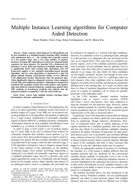
Figure 1 illustrates the idea using a graphical toy example.
In this example there are three positive bags each with five
instances and displayed as circles. The goal is to distinguish
these positive bags from the negative bags, all of which exist
as a single instance and are displayed by the diamonds in the
figure. One of the instances in the positive bags happens to
be an outlier. These are the circles at the right side of the
figure farthest from the rest of the circles. The convex hulls
spanned by the instances of each of the bag are shown with the
polyhedrons in the figure. The MIL algorithm learns a point
within the convex hull of each of the bag (shown with the
stars) while maximizing the margin between the positive and
negative bags. This convex-hull relaxation (first introduced in
[8]) eliminates the combinatorial nature of the MIL problem,
allowing algorithms that are more computationally efficient.
As mentioned above, we will consider that a bag Bi j is
correctly classified if any point inside the convex hull of
the bag Bi j (i.e. any convex combination of points of Bi j )
is correctly classified. Let λ s.t. 0 ≤ λ i j ,e′ λ i j
= 1 be the
vector containing the coefficients of the convex combination
that defines the representative point of bag i in class j. Let r be

TBME-00884-2006.R2 3
1
0.9
0.8
0.7
0.6
0.5
0.4
0.3
0.2
0.1
0
0 0.2 0.4 0.6 0.8 1
Fig. 1. A toy example illustrating the proposed approach. Positive and negative
classes are represented by circles and diamonds respectively. Polyhedrons
represent the convex hulls for the three positives bags, the points chosen by
our algorithm to represent each bag is shown by stars. The gray line represents
the linear hyperplane obtained by our algorithm and the black line represents
the hyperplane for the SVM.
the total number of representative points, i.e. r = r++r−. Let
γ be the total number of convex hull coefficients corresponding
to the representative points in class j, i.e. γj = rj i=1 mij ,
γ = γ+ + γ−. Then, we can formulate the MIL problem as,
min
(ξ,w,η,λ)∈R r+n+1+γ
νE(ξ) + Φ(w,η) + Ψ(λ)
s.t. ξi = di − (λi jBi jw − eη)
ξ ∈ Ω
e ′ λi j = 1
0 ≤ λi j
(1)
Where ξ = {ξ1,...,ξr} are slack terms (errors), η is the bias
(offset from origin) term, and λ is a vector containing all the
λi j for i = 1,...,rj, j ∈ {±}. E : ℜr ⇒ ℜ represents the loss
function, Φ : ℜ (n+1) ⇒ ℜ is a regularization function on the
hyperplane coefficients [14] and Ψ is a regularization function
on the convex combination coefficients λi j . Depending on the
choice of E,Φ,Ψ and Ω, (1) will lead to MIL versions of
several well-known classification algorithms.
1) E(ξ) = (ξ)+ 2
2 , Φ(w,η) = (w,η)2 2 and Ω = ℜr+ ,
leads to MIL versions of the Quadratic-Programming-
SVM [9].
2) E(ξ) = (ξ) 2
2 , Φ(w,η) = (w,η)2 2 and Ω = ℜr ,
leads to MIL versions of the Least-Squares-SVM.
3) ν = 1, E(ξ) = ξ 2
2 , Ω = {ξ : e′ ξj = 0, j ∈ {±}}
leads to MIL versions of the QP formulation for Fisher’s
linear discriminant (FD) [11].
As an example, we derive a special case of the algorithm for
the Fisher’s Discriminant, because this choice (FD) brings us
some algorithmic as well as computational advantages.
B. Convex-Hull MIL for Fisher’s Linear Discriminant
Setting ν = 1, E(ξ) = ξ 2
2 , Ω = {ξ : e′ ξj = 0, j ∈ {±}}
in (1) we obtain the following MIL version of the quadratic
programming algorithm for Fisher’s Linear Discriminant [11].
min
(ξ,w,η,λ)∈R r+n+1+γ
ξ 2
2
+ Φ(w,η) + Ψ(λ)
s.t. ξi = di − (λi jBi jw − eη)
e ′ ξj = 0
e ′ λi j = 1
0 ≤ λi j
The number of variables to be optimized in (2) is r+n+1+γ:
this is computationally infeasible when the number of bags is
large (r > 104 ). To alleviate the situation, we (a) replace ξi by
di − (λi jBi jw − eη) in the objective function, and (b) replace
the equality constraints e ′ ξj = 0 by w ′ (µ+ − µ−) = 2. This
substitution eliminates the variables ξ,η from the problem
and also the corresponding r equality constraints in (2).
Effectively, this results in the MIL version of the traditional FD
algorithm. As discussed later in the paper, in addition to the
obvious computational gains, this manipulation results in some
algorithmic advantages as well (For more information on the
equivalence between the single instance learning versions of
(2) and (3) see [11]). Thus, the optimization problem reduces
to:
min
(w, λ)∈R n+γ
w T SWw + Φ(w) + Ψ(λ)
s.t. wT (µ+ − µ−)
e
= b
′ λi j
0
=
≤
1
λi j
(3)
where SW =
j∈{±} 1
rj (Xj − µje ′ ) (Xj − µje ′ ) T is the
within class scatter matrix, µj = 1
rj Xje is the mean for class
j. Xj ∈ ℜ rj×n is a matrix containing the rj representative
points on n-dimensional space such that the row of Xj denoted
by bi j = Bi jλij is the representative point of bag i in class j
where i = {1,...,rj} and j ∈ {±}.
C. Alternate Optimization for Convex-Hull MIL Fisher’s Discriminant
The proposed mathematical program (3) can be solved using
an efficient Alternate Optimization (AO) algorithm [2]. In the
AO setting the main optimization problem is subdivided in two
smaller or easier subproblems that depend on disjoints subsets
of the original variables. When Φ(w) and Ψ(λ) are strongly
convex functions, both the original obingtive function and the
two subproblems (for optimizing λ and w) in (3) are strongly
convex, meaning that the algorithm converges to a global
minimizer [15]. For computational efficiency, in the remainder
of the paper we will use the regularizers Φ(w) = ǫ w 2
2 and
Ψ(λ) = ǫ λ 2
2 , where ǫ is a positive regularization parameter.
An efficient AO algorithm for solving the mathematical
program (3) is described below.
Sub Problem 1: Fix λ = λ∗ : When we fix λ = λ∗ , the
problem becomes,
min
w∈R n
wT SWw + Φ(w)
s.t. w T (µ+ − µ−) = b
which is the formulation for the Fisher’s Discriminant. Since
SW is the sum of two covariance matrices, it is guaranteed
to be at least positive semidefinite and thus the problem in
(2)
(4)

TBME-00884-2006.R2 4
(4) is convex. For datasets with r >> n, i.e. the number of
bags is much greater than the number of dimensionality, SW is
positive definite and thus the problem in (4) is strictly convex.
Unlike (1) where the number of constraints is proportional to
the number of bags, eliminating ξ and η leaves us with only
one constraint. This changes the order of complexity from
O(nr 2 ) to O(n 2 r) and brings some computational advantages
when dealing with datasets with r >> n.
Sub Problem 2: Fix w = w ∗ : When we fix w = w ∗ , the
problem becomes
min
λ∈R γ
λ T ¯ SWλ + Ψ(λ)
s.t. λT (¯µ+ − ¯µ−) = b
e ′ λi j = 1
0 ≤ λi j
where ¯ SW and ¯µ are defined as in (4) with Xj replaced by
¯Xj where ¯ Xj ∈ ℜ rj×γ is now a matrix containing the rj
new points on the γ-dimensional space such that the row of
¯Xj denoted by ¯b i j is a vector with its nonzero elements set to
B i j w∗ . For the positive class elements i−1
k=1 mk + + 1 through
i
k=1 mk + of ¯ b i j
are nonzero, for the negative class nonzero
elements are located at r+ k=1 mk + + i−1 k=1 mk− + 1 through
r+ k=1 mk + + i k=1 mk−. Note that ¯ SW is also a sum of two
covariance matrices, it is positive semidefinite and thus the
problem in (5) is convex. Unlike sub problem 1 the positive
definiteness of ¯ SW does not depend on the data, since it always
true that r ≤ γ. The complexity of (5) is O(nγ2 ).
As it was mentioned before, in CAD applications, a bag
is defined as a set of candidates that are spatially close
to the radiologist marked ground-truth. Any candidate that
is spatially far from this location is considered negative in
the training data, therefore the concept of bag for negative
examples does not make any practical sense in this scenario.
Moreover, since ground truth is only available on the training
set, there is no concept of a bag on the test set for both
positive and negative examples. The classifier trained in this
framework classifies and labels test instances individually -
the bag information in the training data is only used as a
prior information to obtain a more robust classifier. Hence,
the problem in (5) can be simplified to account for these
practical observations resulting in an optimization problem
with O(nγ2 +) complexity. The entire algorithm is summarized
below for clarity.
D. CH-FD: An Algorithm for Learning Convex Hull Representation
of Multiple Instances
(0) Choose as initial guess for λ i0 = e
m i , ∀i = 1,...,r, set
counter c=0.
(i) For fixed λ ic , ∀i = 1,...,r solve for w c in (4).
(ii) Fixing w = w c solve for λ ic , ∀i = 1,...,r in (5).
(iii) Stop if λ 1(c+1) − λ 1c ,...,λ r(c+1) − λ rc 2 is less than
some desired tolerance. Else replace λ ic by λ i(c+1) and
c by c + 1 and go to (i).
The nonlinear version of the proposed algorithm can be obtained
by first transforming the original datapoints to a kernel
space spanned by all datapoints through a kernel operator, i.e.
(5)
K : ℜ n ⇒ ℜ ¯γ and then by optimizing (4) and (5) in this
new space. Ideally ¯γ is set to γ. However when γ is large, for
computational reasons we can use the technique presented in
[7] to limit the number of datapoints spanning this new space.
This corresponds to constraining w to lie in a subspace of the
kernel space.
III. EXPERIMENTAL RESULTS AND DISCUSSION
For the experiments in section III-A , we compare four
techniques: naive Fisher’s Discriminnat (FD), CH-FD, EM-DD
[16], IDAPR [4]. For IDAPR and EM-DD we used the Matlab
implementation of these algorithms also used in [18]. In both
experiments we used the linear version of our algorithm.
Hence the only parameter that requires tuning is ν which is
tuned to optimize the 10-fold Patient Cross Validation on the
training data,. All algorithms are trained on the training data
and then tested on the sequestered test data. The resulting
Receiver Operating Characteristics (ROC) plots are obtained
by trying different values of the parameters (τ,ǫ) for IDAPR,
and by thresholding the corresponding output for each of the
EM-DD, FD and CH-FD.
A. Two CAD Datasets: Pulmonary Embolism & Colon Cancer
Detection
Next, we present the problems that mainly motivated this
work. Pulmonary embolism (PE), a potentially life-threatening
condition, is a result of underlying venous thromboembolic
disease. An early and accurate diagnosis is the key to survival.
Computed tomography angiography (CTA) has emerged as
an accurate diagnostic tool for PE, and However, there are
hundreds of CT slices in each CTA study and manual reading
is laborious, time consuming and complicated by various
PE look-alikes. Several CAD systems are being developed
to assist radiologists to detect and characterize emboli [12],
[17]. At four different hospitals (two North American sites
and two European sites), we collected 72 cases with 242
PE bags comprised of 1069 positive candidates marked by
expert chest radiologists. The cases were randomly divided
into two sets: training (48 cases with 173 PE bags and 3655
candidates) and testing (24 cases with 69 PE bags and 1857
candidates). The test group was sequestered and only used
to evaluate the performance of the final system. A combined
total of 70 features are extracted for each candidate. These
features were all image-based features and were normalized
to a unit range, with a feature-specific mean. The features can
be categorized into those that are indicative of voxel intensity
distributions within the candidate, those summarizing distributions
in neighborhood of the candidate, and those that describe
the 3-D shape of the candidate and enclosing structures. When
combined these features can capture candidate properties that
can disambiguate typical false positives such as dark areas that
result from poor mixing of bright contrast agents with blood in
veins, and dark connective tissues between vessels, from true
emboli. These features are not necessarily independent, and
may be correlated with each other, especially with features in
the same group.

TBME-00884-2006.R2 5
Colorectal cancer is the third most common cancer in both
men and women. It is estimated that in 2004, nearly 147,000
cases of colon and rectal cancer will be diagnosed in the US,
and more than 56,730 people would die from colon cancer
[5]. CT colonography is emerging as a new procedure to help
in early detection of colon polyps. However, reading through
a large CT dataset, which typically consists of two CT series
of the patient in prone and supine positions, each with several
hundred slices, is time-consuming. Colon CAD [3] can play
a critical role to help the radiologist avoid the missing of
colon polyps. Most polyps, therefore, are represented by two
candidates; one obtained from the prone view and the other
one from the supine view. Moreover, for large polyps, a typical
candidate generation algorithm generates several candidates
across the polyp surface. The database of high-resolution CT
images used in this study were obtained from seven different
sites across US, Europe and Asia. The 188 patients were
randomly partitioned into two groups, training comprised of:
65 cases with 127 volumes, 50 polyps bags (179 positive
candidates) were identified in this set with a total number of
6569 negative candidates and testing comprised of 123 patients
with 237 volumes, a total of 103 polyp bags (232 positive
candidates) were identified in this set with a total number of
12752 negative candidates. The test group was sequestered and
only used to evaluate the performance of the final system.
A total of 75 features are extracted for each candidate. Three
imaging scientists contributed to this stage. These features can
be grouped into three. The first group of features are derived
from properties of patterns of curvature to characterize the
shape, size, texture, density and symmetry. These features
aim at capturing a general class of mostly symmetrical and
round structures protruding inward into the lumen (air within
the colon), having smooth surface and density and texture
characteristics of muscle tissue. These kinds of structures
exhibit symmetrical change of curvature sign about a central
axis perpendicular to the objects surface. Colonic folds, on
the other hand, have shapes that can be characterized as halfcylinders
or paraboloids and hence do not present similar
symmetry about a single axis [6]. The second group of features
are based on a concept called tobogganing. Fast Tobogganing
aims to quickly form a toboggan cluster, which contains the
given pixel without scanning the whole volume. It consists
of two steps; for a given point the algorithm slides/climbs to
its concentration and then expands from the concentration to
form a toboggan cluster. The third group of features are based
on a concept called diverging gradient. In this technique first
the gradient field of the image is computed. Then a filter is
convolved with the gradient field at different scales to generate
multiple response images. Features are extracted by further
processing of these response images at different scales.
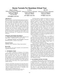
The resulting Receiver Operating Characteristics (ROC)
curves are displayed in Figure 2. Although for the PE dataset
Figure 2 (left) IDAPR crosses over CH-FD and is more
sensitive than CH-FD for extremely high number of false
positives, Table I show that CH-FD is more accurate than all
other methods over the entire space (AUC). Note that CAD
performance is only valid in the clinically acceptable range,
< 10fp/patient for PE, < 5fp/volume for Colon (generally
there are 2 volumes per patient). In the region of clinical
interest (AUC-RCI), Table I shows that CH-FD significantly
outperforms all other methods.
Execution times for all the methods tested are shown in
Table I. As expected, the computational cost is the cheapest
for the traditional non-MIL based FD. Among MIL algorithms,
for the PE data, CH-FD was roughly 2-times and 9-times as
fast than IAPR and EMDD respectively, and for the much
larger colon dataset was roughly 85-times and 2000-times
faster, respectively(see Table I).
Sensitivity
Sensitivity
1
0.9
0.8
0.7
0.6
0.5
0.4
0.3
0.2
0.1
EMDD
IAPR
CH−FD
FD
0
0 10 20 30
FP/Patient
40 50 60
1
0.9
0.8
0.7
0.6
0.5
0.4
0.3
0.2
0.1
CH−FD
EMDD
IAPR
FD
0
0 10 20 30
False positive per volume
40 50 60
Fig. 2. ROC curves obtained for (up) PE Testing data and (down) COLON
testing Data
B. Experiments on Benchmark Datasets
We compare CH-FD with several state-of-the-art MIL algorithms
on 5 benchmark MIL datasets: 2 Musk datasets [4]
and 3 Image Annotation datasets [1]. Each of these datasets
contain both positive and negative bags. CH-FD (and MICA)
use just the positive bag information and ignore the negative
bag information, in effect, treating each negative instance as
a separate bag. All the other MIL algorithms use both the
positive and negative bag information.
The Musk datasets contains feature vectors describing the
surfaces of low-energy shapes from molecules. Each feature
vector has 166 features. The goal is to differentiate molecules

TBME-00884-2006.R2 6
TABLE I
COMPARISON OF 3 MIL AND ONE TRADITIONAL ALGORITHMS: COMPUTATION TIME, AUC, AND NORMALIZED AUC IN THE REGION OF CLINICAL
INTEREST FOR PE AND COLON TEST DATA
Algorithm Time (PE) Time (Colon) AUC (PE) AUC (Colon) AUC-RCI (PE) AUC-RCI (Colon)
IAPR 184.6 689.0 0.83 0.70 0.34 0.26
EMDD 903.5 16614.0 0.67 0.80 0.17 0.42
CH-FD 97.2 7.9 0.86 0.90 0.50 0.69
FD 0.19 0.4 0.74 0.88 0.44 0.57
that smell ”musky” from the rest of the molecules. Approximately
half of the molecules are known to smell musky. There
are two musk datasets. MUSK1 contains 92 molecules with a
total of 476 instances. MUSK2 contains 102 molecules with a
total of 6598 instances. 72 of the molecules are shared between
two datasets but MUSK2 dataset contain more instances for
the shared molecules. The Image Annotation data is composed
of three different categories, . Each dataset namely Tiger,
Elephant, Foxhas 100 positive bags and 100 negative bags.
We set Φ(w) = ν |λ|. For the musk datasets our results
are based on a Radial Basis Function (RBF) kernel
K(xi,xj) = exp(−σ x − y 2 ). The kernel space is assumed
to be spanned by all the datapoints in MUSK1 dataset and a
subset of the datapoints in MUSK2 dataset (one tenth of the
original training set is randomly selected for this purpose).
The width of the kernel function and ν are tuned over a
discrete set of five values each to optimize the 10-fold Cross
Validation performance. For the Image Annotation data we use
the linear version of our algorithm. We follow the benchmark
experiment design and report average accuracy of 10 runs of
10-fold Cross Validation in Table II. Results for other MIL
algorithms from the literature are also reported in the same
table. Iterated Discriminant APR (IAPR), Diverse Density
(DD) [10], Expectation-Maximization Diverse Density (EM-
DD) [16], Maximum Bag Margin Formulation of SVM (mi-
SVM, MI-SVM) [1], Multi Instance Neural Networks (MI-
NN) [13] are the techniques considered in this experiment for
comparison purposes. Results for mi-SVM, MI-SVM and EM-
DD are taken from [1].
Table II shows that CH-FD is comparable to other techniques
on all datasets, even though it ignores the negative
bag information. Furthermore, CH-FD appears to be the most
stable of the algorithms, at least on these 5 datasets, achieving
the most consistent performance as indicated by the ”Average
Rank” column. We believe that this stable behavior of our algorithm
is due in part because it converges to global solutions
avoiding the local minima problem.
IV. CONCLUSIONS
This paper makes three principal contributions. First, we
have identified the need for multiple-instance learning in CAD
applications and described the spatial proximity based intersample
correlations in the label noise for classifier design in
this setting. Second, building on an intuitive convex-relaxation
of the original MIL problem, this paper presents a new approach
to multiple-instance learning. In particular, we dramatically
improve the run time by replacing a large set of discrete
constraints (at least one instance in each bag has to be correctly
classified) with infinite but continuous sets of constraints (at
least one convex combination of the original instances in every
bag has to be correctly classified). Further, the proposed idea
for achieving convexity in the objective function of the training
algorithm alleviates the problems of local maxima that occurs
in some of the previous MIL algorithms, and often improves
the classification accuracy on many practical datasets. Third,
we present a practical implementation of this idea in the form
of a simple but efficient alternate-optimization algorithm for
Convex Hull based Fisher’s Discriminant. In our benchmark
experiments, the resulting algorithm achieves accuracy that is
comparable to the current state of the art, but at a significantly
lower run time (typically several orders of magnitude speed
ups were observed).
ACKNOWLEDGMENT
We would like to thank everyone who contributed to the
Colon and PE CAD projects. Our special thanks goes to Dr.
Sarang Lakare, Dr. Anna Jerebko, Dr. Senthil Periaswamy, Dr.
Liang Jianming and Dr. Luca Bogoni.
REFERENCES
[1] S. Andrews, I. Tsochantaridis, and T. Hofmann, “Support vector machines
for multiple-instance learning,” in Advances in Neural Information
Processing Systems 15, S. T. S. Becker and K. Obermayer, Eds.
Cambridge, MA: MIT Press, 2003, pp. 561–568.
[2] J. Bezdek and R. Hathaway, “Convergence of alternating optimization,”
Neural, Parallel Sci. Comput., vol. 11, no. 4, pp. 351–368, 2003.
[3] L. Bogoni, P. Cathier, M. Dundar, A. Jerebko, S. Lakare, J. Liang,
S. Periaswamy, M. Baker, and M. Macari, “Cad for colonography: A
tool to address a growing need,” British Journal of Radiology, vol. 78,
pp. 57–62, 2005.
[4] T. G. Dietterich, R. H. Lathrop, and T. Lozano-Perez, “Solving
the multiple instance problem with axis-parallel rectangles,” Artificial
Intelligence, vol. 89, no. 1-2, pp. 31–71, 1997. [Online]. Available:
citeseer.ist.psu.edu/dietterich97solving.html
[5] D. Jemal, R. Tiwari, T. Murray, A. Ghafoor, A. Saumuels, E. Ward,
E. Feuer, and M. Thun, “Cancer statistics,” CA Cancer J. Clin., vol. 54,
pp. 8–29, 2004.
[6] A. Jerebko, S. Lakare, P. Cathier, S. Periaswamy, and
L. Bogoni, “Symmetric curvature patterns for colonic
polyp detection,” in Proceedings of the 14th European
Conference on Machine Learning, LNAI 2837. Copenhagen,
Denmark: Springer, 2006, pp. 169–176. [Online]. Available:
http://www.sigmod.org/dblp/db/conf/miccai/miccai2006-2.html
[7] Y.-J. Lee and O. L. Mangasarian, “RSVM: Reduced support vector
machines,” Data Mining Institute, Computer Sciences Department,
University of Wisconsin, Madison, Wisconsin, Tech. Rep. 00-
07, July 2000, proceedings of the First SIAM International Conference
on Data Mining, Chicago, April 5-7, 2001, CD-ROM Proceedings.
ftp://ftp.cs.wisc.edu/pub/dmi/tech-reports/00-07.ps.
[8] O. Mangasarian and E. Wild, “Multiple instance classification via successive
linear programming,” Data Mining Institute, Computer Sciences
Department, University of Wisconsin, Madison, Wisconsin, Tech. Rep.
05–02, 2005.

TBME-00884-2006.R2 7
TABLE II
AVERAGE ACCURACY ON BENCHMARK DATASETS. THE NUMBER IN PARENTHESIS REPRESENTS THE RELATIVE RANK OF EACH OF THE ALGORITHMS
(PERFORMANCE-WISE) IN THE CORRESPONDING DATASET
Datasets MUSK1 MUSK2 Elephant Tiger Fox Average Rank
CH-FD 88.8 (2) 85.7 (2) 82.4 (2) 82.2 (2) 60.4 (2) 2
IAPR 87.2 (5) 83.6 (6) - (-) - (-) - (-) 5.5
DD 88.0 (3) 84.0 (5) - (-) - (-) - (-) 4
EMDD 84.8 (6) 84.9 (3) 78.3 (5) 72.1 (5) 56.1 (5) 4.8
mi-SVM 87.4 (4) 83.6 (6) 82.2 (3) 78.4 (4) 58.2 (3) 4
MI-SVM 77.9 (8) 84.3 (4) 81.4 (4) 84.0 (1) 57.8 (4) 4.2
MI-NN 88.9 (1) 82.5 (7) - (-) - (-) - (-) 4
MICA 84.4 (7) 90.5 (1) 82.5 (1) 82.0(3) 62.0(1) 3.25
[9] O. L. Mangasarian, “Generalized support vector machines,” in Advances
in Large Margin Classifiers, A. Smola, P. Bartlett, B. Schölkopf, and
D. Schuurmans, Eds. Cambridge, MA: MIT Press, 2000, pp. 135–146,
ftp://ftp.cs.wisc.edu/math-prog/tech-reports/98-14.ps.
[10] O. Maron and T. Lozano-Pérez, “A framework for multipleinstance
learning,” in Advances in Neural Information Processing
Systems 10, M. I. Jordan, M. J. Kearns, and S. A. Solla, Eds.,
vol. 10. Cambridge, MA: MIT Press, 1998. [Online]. Available:
citeseer.ist.psu.edu/maron98framework.html
[11] S. Mika, G. Rätsch, and K. R. Müller, “A mathematical programming
approach to the kernel fisher algorithm,” in Advances in Neural
Information Processing Systems 12, 2000, pp. 591–597. [Online].
Available: citeseer.ist.psu.edu/mika01mathematical.html
[12] M. Quist, H. Bouma, C. V. Kuijk, O. V. Delden, and F. Gerritsen,
“Computer aided detection of pulmonary embolism on multi-detector
ct,” in Proceedings of the 90th meeting of the Radiological Society of
North America (RSNA), 2004.
[13] J. Ramon and L. D. Raedt, “Multi instance neural
networks,” in Proceedings of ICML-2000 workshop on Attribute-
Value and Relational Learning., 2000. [Online]. Available:
citeseer.ist.psu.edu/ramon00multi.html
[14] V. N. Vapnik, The Nature of Statistical Learning Theory. New York:
Springer, 1995.
[15] J. Warga, “Minimizing certain convex functions,” Journal of SIAM on
Applied Mathematics, vol. 11, pp. 588–593, 1963.
[16] Q. Zhang and S. Goldman, “Em-dd: An improved multiple-instance
learning technique,” in Advances in Neural Information Processing
Systems 14, T. G. Dietterich, S. Becker, and Z. Ghahramani, Eds.,
vol. 14. Cambridge, MA: MIT Press, 2001, pp. 1073–1080. [Online].
Available: citeseer.ist.psu.edu/article/zhang01emdd.html
[17] C. Zhou, L. M. Hadjiiski, B. Sahiner, H.-P. Chan, S. Patel, P. Cascade,
E. A. Kazerooni, and J. Wei, “Computerized detection of pulmonary
embolism in 3D computed tomographic (CT) images: vessel tracking
and segmentation techniques,” in Medical Imaging 2003: Image Processing.
Edited by Sonka, Milan; Fitzpatrick, J. Michael. Proceedings of the
SPIE, Volume 5032, pp. 1613-1620 (2003)., May 2003, pp. 1613–1620.
[18] Z. Zhou and M. Zhang, “Ensembles of multi-instance learners,” in
Proceedings of the 14th European Conference on Machine Learning,
LNAI 2837. Cavtat-Dubrovnik, Croatia: Springer, 2003, pp. 492–502.
[Online]. Available: citeseer.ist.psu.edu/zhou03ensembles.html
Dr. M. Murat Dundar received his B.Sc. degree
from Bogazici University Istanbul, Turkey, in 1997
and his M.S. and Ph.D. degrees from Purdue University
in 1999 and 2003 respectively, all in Electrical
Engineering. Since 2003 he works as a scientist
in Siemens Medical Solutions, USA. His research
interests include statistical pattern recognition and
computational learning with applications to computer
aided detection, hyperspectral data analysis
and remote sensing.
Dr. Glenn Fung received B.S. degree in pure
mathematics from Universidad Lisandro Alvarado
in Barquisimeto, Venezuela, then earned an M.S. in
applied mathematics from Universidad Simon Bolivar,
Caracas, Venezuela where later he worked as
an assistant professor for two years. He also earned
an M.S. degree and a Ph. D. degree in computer
sciences from the University of Wisconsin-Madison.
His main interests are Optimization approaches to
Machine Learning and Data Mining, with emphasis
in Support Vector Machines. In the summer of 2003
he joined the computer aided diagnosis group at Siemens, medical solutions
in Malvern, PA where he has been applying Machine learning techniques to
solve challenging problems that arise in the medical domain. His recent papers
are available at www.cs.wisc.edu/ gfung.
Dr. Balaji Krishnapuram received his B. Tech.
from the Indian Institute of Technology (IIT)
Kharagpur, in 1999 and his PhD from Duke University
in 2004, both in Electrical Engineering. He
works as a scientist in Siemens Medical Solutions,
USA. His research interests include statistical pattern
recognition, Bayesian inference and computational
learning theory. He is also interested in applications
in computer aided medical diagnosis, signal processing,
computer vision and bioinformatics.
Dr. R. Bharat Rao is the Senior Director of Engineering
R&D, at the Computer-Aided Diagnosis
and Knowledge Solutions (CKS) Solutions Group
in Siemens Medical Solutions, Malvern, PA. He
received his Ph.D. in machine learning from the
Department of Electrical & Computer Engineering,
University of Illinois, Urbana-Champaign, in 1993.
Dr. Rao joined Siemens Corporate Research in 1993,
and managed the Data Mining group over there from
1996. In 2002, he joined the then-formed Computer-
Aided Diagnosis & Therapy Group in Siemens Medical
Solutions, with a particular focus on using clinical patient information
and data mining methods to help improve traditional computer-aided detection
methods. In 2005, Siemens honored him with its ”Inventor of the Year” award
for outstanding contributions related to improving the technical expertise and
the economic success of the company. He also received the inaugural IEEE
Data Mining Practice Prize for the best deployed industrial and government
data mining application in 2005.
His current research interests are focused on the use of machine learning
and probabilistic inference to develop decision-support tools that can help
physicians improve the quality of patient care and their efficiency. He is
particularly interested in the development of novel data mining methods to
collectively mine and integrate the various parts of a patient record (lab tests,
pharmacy, free text, images, proteomics, etc.) and the integration of medical
knowledge into the mining process.