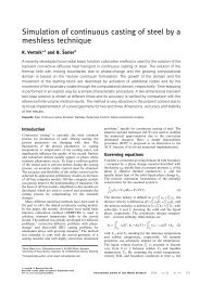
Numerical Modeling of Grain Structure in Continuous Casting of Steel
Numerical Modeling of Grain Structure in Continuous Casting of Steel
Numerical Modeling of Grain Structure in Continuous Casting of Steel

You also want an ePaper? Increase the reach of your titles
YUMPU automatically turns print PDFs into web optimized ePapers that Google loves.
Copyright c○ 2009 Tech Science Press CMC, vol.8, no.3, pp.195-208, 2009<br />
<strong>Numerical</strong> <strong>Model<strong>in</strong>g</strong> <strong>of</strong> <strong>Gra<strong>in</strong></strong> <strong>Structure</strong> <strong>in</strong> Cont<strong>in</strong>uous Cast<strong>in</strong>g <strong>of</strong> <strong>Steel</strong><br />
A.Z. Lorbiecka 1 , R.Vertnik 2 , H.Gjerkeš 1 , G. Manojlovič 2 ,B.Senčič 2<br />
J. Cesar 2 and B.Šarler 1,3<br />
Abstract: A numerical model is developed for<br />
the simulation <strong>of</strong> solidification gra<strong>in</strong> structure formation<br />
(equiaxed to columnar and columnar to<br />
equiaxed transitions) dur<strong>in</strong>g the cont<strong>in</strong>uous cast<strong>in</strong>g<br />
process <strong>of</strong> steel billets. The cellular automata<br />
microstructure model is comb<strong>in</strong>ed with<br />
the macroscopic heat transfer model. The cellular<br />
automata method is based on the Nastac’s def<strong>in</strong>ition<br />
<strong>of</strong> neighborhood, Gaussian nucleation rule,<br />
and KGT growth model. The heat transfer model<br />
is solved by the meshless technique by us<strong>in</strong>g local<br />
collocation with radial basis functions. The microscopic<br />
model parameters have been adjusted<br />
with respect to the experimental data for steel<br />
51CrMoV4. Simulations have been carried out<br />
for nom<strong>in</strong>al cast<strong>in</strong>g conditions, reduced cast<strong>in</strong>g<br />
temperature, and reduced cast<strong>in</strong>g speed. Proper<br />
response <strong>of</strong> the multiscale model with respect to<br />
the observed gra<strong>in</strong> structures has been proved.<br />
Keyword: cont<strong>in</strong>uous cast<strong>in</strong>g <strong>of</strong> steel, solidification,<br />
multiscale model<strong>in</strong>g, equiaxed to columnar<br />
transition, columnar to equiaxed transition,<br />
macroscopic model, microscopic model, heat<br />
transfer model, cellular automata model, meshless<br />
methods.<br />
1 Introduction<br />
An important and huge class <strong>of</strong> manufactur<strong>in</strong>g<br />
and materials process<strong>in</strong>g operations <strong>in</strong>clude solidification<br />
<strong>of</strong> metals at some stage. Among these<br />
is the process <strong>of</strong> cont<strong>in</strong>uous cas<strong>in</strong>g <strong>of</strong> steel [Irw<strong>in</strong>g,<br />
(1993)] most wide spread. The properties<br />
<strong>of</strong> the cont<strong>in</strong>uously cast billets, slabs and<br />
blooms <strong>in</strong> downstream process<strong>in</strong>g are strongly<br />
1 Laboratory for Multiphase Processes, University <strong>of</strong> Nova<br />
Gorica, Slovenia<br />
2 Štore <strong>Steel</strong> Company, d.o.o. Štore, Slovenia<br />
3 Correspond<strong>in</strong>g author. Email: bozidar.sarler@p-ng.si<br />
affected by the microstructural features and different<br />
types <strong>of</strong> defects, such as cracks, porosity<br />
and macrosegregation. There is a grow<strong>in</strong>g <strong>in</strong>terest<br />
<strong>in</strong> computational model<strong>in</strong>g <strong>of</strong> cont<strong>in</strong>uous<br />
cast<strong>in</strong>g <strong>of</strong> steel [Thomas (2001); Šarler, Vertnik,<br />
Šaletić, Manojlović and Cesar (2005)], <strong>in</strong> order<br />
to be able to predict the properties <strong>of</strong> the product.<br />
The properties <strong>of</strong> the product can be calculated<br />
[Janssens, Raabe, Kozeschnik, Miodownik<br />
and Nestler (2007)] through a comb<strong>in</strong>ation <strong>of</strong><br />
the macroscopic and microscopic models. The<br />
macroscopic model calculates the relations between<br />
the process parameters and the macroscopic<br />
variables, such as temperatures, concentrations,<br />
and velocities on the scale <strong>of</strong> the process.<br />
The microscopic model calculates the relations<br />
between the macroscopic variables and<br />
the microstructure. The properties <strong>of</strong> the product<br />
can be related afterwards from the microstructure.<br />
The multiscale model<strong>in</strong>g [Shen and Atluri (2004);<br />
Haasemann, Kästner and Ulbricht (2006); Zhang<br />
and Shen (2008)] represents one <strong>of</strong> the currently<br />
most rapidly develop<strong>in</strong>g computational mechanics<br />
fields.<br />
A pr<strong>in</strong>cipal goal <strong>of</strong> this study represents the development<br />
<strong>of</strong> a new simulation tool for model<strong>in</strong>g<br />
the dendritic gra<strong>in</strong> structure <strong>in</strong> solidification<br />
<strong>of</strong> steel (equiaxed to columnar transition (ECT)<br />
and columnar to equiaxed transition (CET)) by<br />
us<strong>in</strong>g coupled micro and macroscopic models and<br />
validation <strong>of</strong> the model by experimental results.<br />
Several stochastic models <strong>of</strong> microstructure have<br />
been developed over the past years. The first approach<br />
was <strong>in</strong>itiated by Spittle and Brown [Spittle<br />
and Brown (1989)], based on the Monte Carlo<br />
procedure to predict re-crystallization and gra<strong>in</strong><br />
growth <strong>in</strong> the solid – solid phase transformations,<br />
as well as to simulate the solidification structure.<br />
Rappaz and Gand<strong>in</strong> [Rappaz and Gand<strong>in</strong> (1993)]
196 Copyright c○ 2009 Tech Science Press CMC, vol.8, no.3, pp.195-208, 2009<br />
were the first who applied another stochastic<br />
model, the Cellular Automata (CA) technique to<br />
predict solidification gra<strong>in</strong> structure.<br />
The present paper is structured <strong>in</strong> the follow<strong>in</strong>g<br />
way: we present macroscopic and microscopic<br />
models first, followed by the description<br />
<strong>of</strong> the determ<strong>in</strong>istic and stochastic solution procedures.<br />
The experimental validation <strong>of</strong> the model<br />
describes next. F<strong>in</strong>ally, we represent the <strong>in</strong>fluence<br />
<strong>of</strong> the process parameters on the gra<strong>in</strong> structure <strong>of</strong><br />
the cont<strong>in</strong>uously cast billet.<br />
2 Macroscopic model<br />
The macroscopic model is designed to be able<br />
to calculate the steady temperature distribution <strong>in</strong><br />
the cont<strong>in</strong>uously cast billet as a function <strong>of</strong> the<br />
follow<strong>in</strong>g process parameters: billet dimension,<br />
steel grade, cast<strong>in</strong>g temperature, cast<strong>in</strong>g velocity,<br />
primary and two secondary cool<strong>in</strong>g systems<br />
flows, pressures, temperatures, type and quantity<br />
<strong>of</strong> the cast<strong>in</strong>g powder, and the (non)application<br />
<strong>of</strong> the radiation shield and electromagnetic stirr<strong>in</strong>g.<br />
The Bennon-Incropera [Bennon and Incropera<br />
(1987)] mixture cont<strong>in</strong>uum formulation is<br />
used for the physical model, solved by the recently<br />
developed meshless Local Radial Basis<br />
Function Collocation Method (LRBFCM) [Šarler<br />
and Vertnik (2006); Vertnik and Šarler (2006);<br />
Vertnik, Založnik and Šarler (2006)]. In this novel<br />
numerical method, the doma<strong>in</strong> and boundary <strong>of</strong><br />
<strong>in</strong>terest are divided <strong>in</strong>to overlapp<strong>in</strong>g <strong>in</strong>fluence areas.<br />
On each <strong>of</strong> them, the fields are represented<br />
by the multiquadrics radial basis function collocation<br />
on a related sub-set <strong>of</strong> nodes. Time-stepp<strong>in</strong>g<br />
is performed <strong>in</strong> an explicit way. The govern<strong>in</strong>g<br />
equations are solved <strong>in</strong> its strong form, i.e. no<br />
<strong>in</strong>tegrations are performed. The polygonization<br />
is not present and the method is practically <strong>in</strong>dependent<br />
on the problem dimension. The other<br />
possibility represents the local approximation by<br />
the mov<strong>in</strong>g least squares [Šarler, Vertnik, Perko<br />
(2005)] <strong>in</strong>stead <strong>of</strong> <strong>in</strong>terpolation.<br />
The convergence, cont<strong>in</strong>uity, and completeness <strong>of</strong><br />
global radial basis function <strong>in</strong>terpolation, based<br />
on the multiquadrics, has been recently elaborated<br />
by [Huang, Lee and Cheng (2007)]. A related<br />
comprehensive mathematical study is given<br />
<strong>in</strong> [Buhmann (2003)]. At the present state-<strong>of</strong>-theart,<br />
no rigorous mathematical theory exists for the<br />
local collocation. Nevertheless, the convergence<br />
<strong>of</strong> the method has been demonstrated for diffusion<br />
problems on NAFEMS [Cameron, Casey,<br />
Simpson (1986)] benchmark test and Dirichlet<br />
jump problem, and compared to the f<strong>in</strong>ite difference<br />
method (FDM) [Šarler and Vertnik (2006)].<br />
The favorable convergence <strong>of</strong> the method compared<br />
to the classical second order FDM was<br />
demonstrated. The convergence <strong>of</strong> the LRBFCM<br />
was tested for convective-diffusive problems with<br />
and without phase change <strong>in</strong> [Vertnik and Šarler<br />
(2006)] and compared with the boundary element<br />
and f<strong>in</strong>ite element methods. Favorable convergence<br />
properties <strong>of</strong> the LRBFCM have been<br />
demonstrated <strong>in</strong> this case as well. The RBFbased<br />
numerical methods represent one <strong>of</strong> the<br />
key directions <strong>in</strong> meshless methods research for<br />
fluids [Amaziane, Naji and Ouazar (2004); Šarler<br />
(2005); Mai-Duy, Mai-Cao and Tran-Cong<br />
(2007); Divo and Kassab (2007); Kosec and Šarler<br />
(2008)], solids [Mai-Duy, Khennane and Tran-<br />
Cong (2007); Le, Mai-Dui, Tran-Cong and Baker<br />
(2008)], mov<strong>in</strong>g boundaries [La Rocca, Power,<br />
La Rocca and Morale (2005); Mai-Cao and Tran-<br />
Cong (2008)] and solution <strong>of</strong> partial differential<br />
menthods <strong>in</strong> general [Mai-Duy and Tran-Cong<br />
(2003); Mai-Cao and Tran-Cong (2005)].<br />
2.1 Govern<strong>in</strong>g equations<br />
Consider a connected fixed doma<strong>in</strong> Ω with<br />
boundary Γ occupied by a liquid-solid phase<br />
change material described with the temperature<br />
dependent density ρ℘ <strong>of</strong> the phase ℘, temperature<br />
dependent specific heat at constant pressure<br />
c℘, thermal conductivity k℘, and the specific latent<br />
heat <strong>of</strong> the solid-liquid phase change hm. The<br />
mixture cont<strong>in</strong>uum formulation [Bennon and Incropera<br />
(1987)] <strong>of</strong> the enthalpy conservation for<br />
the assumed system is<br />
∂<br />
(ρh)+∇· (ρvh)=∇· (k∇T )<br />
∂t<br />
+∇· ρvh − f V S ρSvShS − f V <br />
L ρLvLhL (1)<br />
where the second term on the right-hand side is<br />
a correction term, needed to accommodate the
<strong>Numerical</strong> <strong>Model<strong>in</strong>g</strong> <strong>of</strong> <strong>Gra<strong>in</strong></strong> <strong>Structure</strong> <strong>in</strong> Cont<strong>in</strong>uous Cast<strong>in</strong>g <strong>of</strong> <strong>Steel</strong> 197<br />
mixture cont<strong>in</strong>uum formulation <strong>of</strong> the convective<br />
term. In cont<strong>in</strong>uation we neglect this term. In Eq.<br />
(1) mixture density and thermal conductivity are<br />
def<strong>in</strong>ed as<br />
ρ = f V S ρS + f V L ρL, (2)<br />
k = f V S kS + f V L kL, (3)<br />
where f V ℘ represents the volume fraction <strong>of</strong> the<br />
phase ℘. The liquid volume fraction f V L might<br />
vary from 0 to 1 between solidus TS and liquidus<br />
temperature TL. Mixture velocity is def<strong>in</strong>ed as<br />
v = f V S ρSvS + f V <br />
L ρLvL /ρ, (4)<br />
and mixture enthalpy is def<strong>in</strong>ed as<br />
h = f V S hS + f V L hL. (5)<br />
The constitutive temperature-enthalpy relationships<br />
are<br />
T<br />
hS = cSdT, (6)<br />
Tre f<br />
T<br />
hL = hS (T )+ (cL −cS)dT +hm,<br />
TS<br />
(7)<br />
with Tre f stand<strong>in</strong>g for the reference temperature.<br />
Thermal conductivity and specific heat <strong>of</strong> the<br />
phases can arbitrarily depend on temperature.<br />
2.2 Spatial discretization<br />
The temperature field <strong>of</strong> a po<strong>in</strong>t <strong>in</strong> the billet is prescribed<br />
by the follow<strong>in</strong>g three-dimensional vector<br />
<strong>in</strong> the Cartesian coord<strong>in</strong>ate system:<br />
p = xix +yiy +ziz, (8)<br />
where x, y, z are coord<strong>in</strong>ates and ix, iy, iz are base<br />
vectors. The z coord<strong>in</strong>ate measures the length<br />
<strong>of</strong> the <strong>in</strong>ner radius <strong>of</strong> the cast<strong>in</strong>g mach<strong>in</strong>e. This<br />
Cartesian coord<strong>in</strong>ate system represents the flat geometry,<br />
which is the geometrical approximation<br />
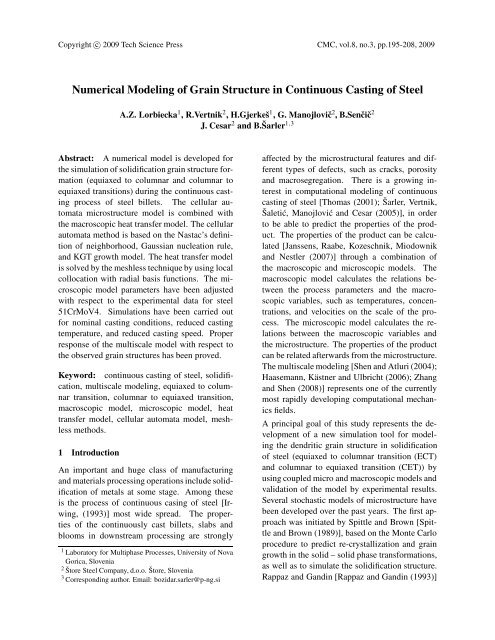
<strong>of</strong> the real curved cast<strong>in</strong>g process (Fig. 1). The<br />
orig<strong>in</strong> <strong>of</strong> the z coord<strong>in</strong>ate co<strong>in</strong>cides with the the<br />
top side <strong>of</strong> the mould, and the base vector iz co<strong>in</strong>cides<br />
with the cast<strong>in</strong>g direction. The x coord<strong>in</strong>ate<br />
measures the width (west-east direction) <strong>of</strong><br />
the billet, perpendicular to the cast<strong>in</strong>g direction.<br />
Its orig<strong>in</strong> co<strong>in</strong>cides with the centre <strong>of</strong> the billet.<br />
The y coord<strong>in</strong>ate measures the thickness (southnorth<br />
direction) <strong>of</strong> the billet, perpendicular to the<br />
cast<strong>in</strong>g direction. Its orig<strong>in</strong> co<strong>in</strong>cides with the <strong>in</strong>ner<br />
(south) side <strong>of</strong> the billet.<br />
Accord<strong>in</strong>g to the heat transfer phenomena <strong>of</strong> the<br />
cont<strong>in</strong>uous cast<strong>in</strong>g <strong>of</strong> steel, the heat conduction <strong>in</strong><br />
the cast<strong>in</strong>g direction might be roughly neglected.<br />
The z coord<strong>in</strong>ate is then parabolic, while the x and<br />
y coord<strong>in</strong>ates are elliptic. The temperature field <strong>in</strong><br />
the billet at a given time is described by the calculation<br />
<strong>of</strong> the cross-section (called <strong>in</strong>f<strong>in</strong>ite slice)<br />
temperature field <strong>of</strong> the billet. In this way the temperature<br />
field at a given z coord<strong>in</strong>ate depends only<br />
on the slice history and its cool<strong>in</strong>g <strong>in</strong>tensity as a<br />
function <strong>of</strong> time. The slices form at the zstart longitud<strong>in</strong>al<br />
coord<strong>in</strong>ate <strong>of</strong> cast<strong>in</strong>g and travel <strong>in</strong> the direction<br />
<strong>of</strong> the iz base vector with the cast<strong>in</strong>g speed<br />
v. For calculat<strong>in</strong>g the cool<strong>in</strong>g <strong>in</strong>tensity <strong>of</strong> the slice<br />
as a function <strong>of</strong> time, we need the connection between<br />
the z coord<strong>in</strong>ate <strong>of</strong> the cast<strong>in</strong>g mach<strong>in</strong>e and<br />
the slice history t, which is <strong>in</strong> general<br />
z(t)=<br />
t<br />
tstart<br />
v(t , )dt , +zstart, v(t)=v (t) · iz, (9)<br />
where tstart is the <strong>in</strong>itial time <strong>of</strong> a slice. In the case<br />
when the cast<strong>in</strong>g speed and other process parameters<br />
are steady, we obta<strong>in</strong> the follow<strong>in</strong>g simple<br />
connection between the z coord<strong>in</strong>ate <strong>of</strong> the cast<strong>in</strong>g<br />
mach<strong>in</strong>e and the slice history t<br />
t (z)=<br />
z −zstart<br />
v<br />
+tstart. (10)<br />
∂<br />
(ρh)=∇· (k∇T ). (11)<br />
∂t<br />
In this paper, the simple Eq. (10) is used, s<strong>in</strong>ce<br />
we assume the steady-state solution <strong>of</strong> the cast<strong>in</strong>g<br />
process. The prescribed simplified spatial discretization<br />
also simplifies the Eq. (1) by remov<strong>in</strong>g<br />
the convective terms. Thus the Eq. (1) transforms<br />
<strong>in</strong>to transient equation, def<strong>in</strong>ed on x-y plane. This<br />
simplified model is consistent with the models,<br />
given by [Louhenkilpi (1995)].<br />
2.3 Boundary conditions<br />
The heat transport mechanisms <strong>in</strong> the mould<br />
take <strong>in</strong>to account the heat transport mechanisms
198 Copyright c○ 2009 Tech Science Press CMC, vol.8, no.3, pp.195-208, 2009<br />
Figure 1: Slice travel<strong>in</strong>g schematics <strong>of</strong> the billet (See Fig. 8 for the slice discretization).<br />
through the cast<strong>in</strong>g powder, across the air-gap (if<br />
it exists), to the mould surface, <strong>in</strong> the mould, and<br />
from the mould <strong>in</strong>ner surface to the mould cool<strong>in</strong>g<br />
water. The heat transport mechanisms <strong>in</strong> the secondary<br />
cool<strong>in</strong>g zone take <strong>in</strong>to account the effects<br />
<strong>of</strong> the cast<strong>in</strong>g velocity, strand surface temperature,<br />
spray nozzle type, spray water flow, temperature<br />
and pressure, radiation and cool<strong>in</strong>g through<br />
the rolls contact. Different types <strong>of</strong> the rolls are<br />
considered (driv<strong>in</strong>g, passive, centrally cooled, externally<br />
cooled, etc.). The mentioned basic heat<br />
transfer mechanisms are modified with regard to<br />
runn<strong>in</strong>g water and rolls stagnant water at relevant<br />
positions. It is not possible to explicitly expose all<br />
the <strong>in</strong>volved correlations with<strong>in</strong> the scope <strong>of</strong> the<br />
present paper. Respectively, the calculated temperature<br />
distributions <strong>of</strong> the macroscopic model<br />
are given <strong>in</strong> Figs. 2-4 for the nom<strong>in</strong>al conditions<br />
and for the reduced cast<strong>in</strong>g temperature and<br />
speed.<br />
2.4 Solution procedure<br />
We seek for mixture temperature at time t0 + Δt<br />
by assum<strong>in</strong>g known <strong>in</strong>itial temperature, velocity<br />
field, and boundary conditions at time t0. The <strong>in</strong>itial<br />
value <strong>of</strong> the temperature T (p,t) at a po<strong>in</strong>t with<br />
position vector p and time t0 is def<strong>in</strong>ed through<br />
the known function T0<br />
T (p,t)=T0 (p);p ∈ Ω +Γ (12)<br />
The boundary Γ is divided <strong>in</strong>to not necessarily<br />
connected parts Γ = Γ D ∪ Γ N ∪ Γ R with Dirichlet,<br />
Neumann and Rob<strong>in</strong> type boundary conditions,<br />
respectively. At the boundary po<strong>in</strong>t p with normal<br />
nΓ and time t0 ≤ t ≤ t0 + Δt, these boundary<br />
conditions are def<strong>in</strong>ed through known functions<br />
T D Γ , T N Γ , T R Γ , T R Γre f<br />
T = T D Γ ;p ∈ Γ D<br />
∂<br />
∂nΓ<br />
∂<br />
∂nΓ<br />
T = T N Γ ;p ∈ Γ N<br />
T = T R Γ<br />
(13)<br />
(14)<br />
R R T −TΓre f ;p ∈ Γ (15)<br />
The numerical discretization <strong>of</strong> Eq. (11), us<strong>in</strong>g<br />
explicit (Euler) time discretization has the form<br />
∂ (ρh)<br />
∂t<br />
≈ ρh −ρ0h0<br />
Δt<br />
= ∇· (k0∇T0) (16)<br />
From Eq. (16) the unknown function value hl <strong>in</strong><br />
doma<strong>in</strong> node pl can be calculated as<br />
hl = h0l + Δt<br />
ρ0c0<br />
(∇k0l · ∇T0l+ k0l · ∇ 2 <br />
T0l<br />
(17)<br />
The spatial derivatives <strong>in</strong> Eq. (17) are approximated<br />
by the LRBFCM. In the LRBFCM, the representation<br />
<strong>of</strong> unknown function value over a set<br />
<strong>of</strong> lN (<strong>in</strong> general) non-equally spaced nodes lpn;<br />
n = 1,2,..., lN is made <strong>in</strong> the follow<strong>in</strong>g way<br />
φ (p) ≈ lK<br />
∑ lψk (p)lαk<br />
k=1<br />
(18)
<strong>Numerical</strong> <strong>Model<strong>in</strong>g</strong> <strong>of</strong> <strong>Gra<strong>in</strong></strong> <strong>Structure</strong> <strong>in</strong> Cont<strong>in</strong>uous Cast<strong>in</strong>g <strong>of</strong> <strong>Steel</strong> 199<br />
where lψk stands for the shape functions, lαk for<br />
the coefficients <strong>of</strong> the shape functions, and lK represents<br />
the number <strong>of</strong> the shape functions. The<br />
left lower <strong>in</strong>dex on entries <strong>of</strong> expression (18) represents<br />
the <strong>in</strong>fluence doma<strong>in</strong> (subdoma<strong>in</strong> or support)<br />
lω on which the coefficients lαk are determ<strong>in</strong>ed.<br />
The <strong>in</strong>fluence doma<strong>in</strong>s lω can <strong>in</strong> general<br />
be contiguous (overlapp<strong>in</strong>g) or non-contiguous<br />
(non-overlapp<strong>in</strong>g). Each <strong>of</strong> the <strong>in</strong>fluence doma<strong>in</strong>s<br />
lω <strong>in</strong>cludes lN nodes <strong>of</strong> which lNΩ can <strong>in</strong> general<br />
be <strong>in</strong> the doma<strong>in</strong> and lNΓ on the boundary, i.e.<br />
lN = lNΩ + lNΓ. The total number <strong>of</strong> all nodes pn<br />
is equal N = NΩ +NΓ <strong>of</strong> which NΓ are located on<br />
the boundary and NΩ are located <strong>in</strong> the doma<strong>in</strong>.<br />
The <strong>in</strong>fluence doma<strong>in</strong> <strong>of</strong> the node lp is def<strong>in</strong>ed<br />
with the nodes hav<strong>in</strong>g the nearest lN −1 distances<br />
to the node lp. The five nodded lN = 5 <strong>in</strong>fluence<br />
doma<strong>in</strong>s are used <strong>in</strong> this paper. The coefficients<br />
are calculated by the collocation (<strong>in</strong>terpolation).<br />
Let us assume the known function values lφn <strong>in</strong><br />
the nodes lpn <strong>of</strong> the <strong>in</strong>fluence doma<strong>in</strong> lω. The<br />
collocation implies<br />
∑<br />
φ (lpn)= lN<br />
k=1<br />
lψk (lpn) lαk. (19)<br />
For the coefficients to be computable, the number<br />
<strong>of</strong> the shape functions has to match the number <strong>of</strong><br />
the collocation po<strong>in</strong>ts lK = lN, and the collocation<br />
matrix has to be non-s<strong>in</strong>gular. The system <strong>of</strong> Eqs.<br />
(19) can be written <strong>in</strong> a matrix-vector notation<br />
lψlα = lΦ; lψkn = lψk (lpn), lφn = φ (lpn).<br />
(20)<br />
The coefficients lα can be computed by <strong>in</strong>vert<strong>in</strong>g<br />
the system (20)<br />
lα = lψ −1 lΦ. (21)<br />
By tak<strong>in</strong>g <strong>in</strong>to account the expressions for the calculation<br />
<strong>of</strong> the coefficients, lα the collocation representation<br />
<strong>of</strong> temperature φ (p) on subdoma<strong>in</strong> lω<br />
can be expressed as<br />
φ (p) ≈ lN<br />
∑<br />
k=1<br />
∑<br />
lψk (p) lN<br />
n=1<br />
lψ −1<br />
kn lφn. (22)<br />
The first partial spatial derivatives <strong>of</strong> φ (p) on subdoma<strong>in</strong><br />
lω can be expressed as<br />
∂<br />
φ (p) ≈<br />
∂ pς<br />
lN<br />
∂<br />
∑ ∂ pς lψk (p) lN<br />
k=1<br />
∑<br />
n=1<br />
lψ −1<br />
kn lφn;<br />
ς = x,y. (23)<br />
The second partial spatial derivatives <strong>of</strong> φ (p) on<br />
subdoma<strong>in</strong> lω can be expressed as<br />
∂ 2<br />
∂ pς pξ φ (p) ≈ lN<br />
∑<br />
∂<br />
k=1<br />
2<br />
lψk (p)<br />
∂ pς pξ lN<br />
∑ lψ<br />
n=1<br />
−1<br />
kn lφn;<br />
ς, ξ = x,y. (24)<br />
The radial basis functions, such as multiquadrics,<br />
can be used for the shape functions<br />
lψk (p)= lr 2 k (p)+c 2 1/2 , (25)<br />
where c represents the shape parameter. These<br />
functions possess C ∞ cont<strong>in</strong>uity and can easily be<br />
used for approximation <strong>of</strong> the <strong>in</strong>volved first and<br />
second order derivatives. The explicit values <strong>of</strong><br />
the <strong>in</strong>volved first and second derivatives <strong>of</strong> ψk (p)<br />
are<br />
∂<br />
∂ pς lψk (p)= pς − l pkς<br />
<br />
lr2 k +c2 , ς = x,y (26)<br />
1/2<br />
∂ 2<br />
∂ p 2 ς<br />
lψk (p)= lr2 k − 2 2<br />
pς − l pkς +c<br />
<br />
lr2 k +c2 , ς = x,y<br />
3/2<br />
(27)<br />
More elaborated step by step description and test<strong>in</strong>g<br />
<strong>of</strong> the present solution procedure for temperature<br />
field is presented <strong>in</strong> [Šarler and Vertnik<br />
(2006)]. A successful comparison <strong>of</strong> the<br />
present meshless solution with the conventional<br />
CFD code Fluent for the cont<strong>in</strong>uous cast<strong>in</strong>g <strong>of</strong><br />
steel is given <strong>in</strong> [Vertnik, Šarler, Buliński and<br />
Manojloviæ (2007)]. The use <strong>of</strong> the model <strong>in</strong><br />
simulation system for cont<strong>in</strong>uous cast<strong>in</strong>g <strong>of</strong> steel<br />
billets is given <strong>in</strong> [Šarler, Vertnik, Gjerkeš, Lorbiecka,<br />
Manojlović, Cesar, Marčič and Sabolič<br />
(2006)].
200 Copyright c○ 2009 Tech Science Press CMC, vol.8, no.3, pp.195-208, 2009<br />
2.5 Macroscopic simulations<br />
Simulations were performed for the billet <strong>of</strong> dimension<br />
140x140 mm and the spr<strong>in</strong>g steel grade<br />
51CrMoV4. The process parameters were taken<br />
directly from the process computer, <strong>in</strong>stalled on<br />
the cast<strong>in</strong>g mach<strong>in</strong>e.<br />
The thermo-physical material properties <strong>of</strong> the<br />
spr<strong>in</strong>g steel were calculated by the JMatPro<br />
s<strong>of</strong>tware [Saunders, Li, Miodownik and Schille<br />
(2003)]. Three simulations have been preprepared<br />
for <strong>in</strong>put <strong>of</strong> the microscopic model (see<br />
details <strong>in</strong> Tab. 1). The numerical results for each<br />
case are presented <strong>in</strong> Figs. 2-4, where the centerl<strong>in</strong>e<br />
and corner temperatures along the cast<strong>in</strong>g<br />
direction are plotted. In each figure, the top l<strong>in</strong>e<br />
represents the centerl<strong>in</strong>e temperature, the middle<br />
l<strong>in</strong>es represent centerl<strong>in</strong>e temperatures <strong>of</strong> the surfaces,<br />
and the bottom l<strong>in</strong>es represent the corner<br />
temperatures.<br />
3 Microscopic model<br />
The follow<strong>in</strong>g three processes take place on the<br />
microstructure level:<br />
• Nucleation process: occurs when a small<br />
gra<strong>in</strong> <strong>of</strong> solid forms <strong>in</strong> the liquid. This is a<br />
k<strong>in</strong>etic process <strong>in</strong> which a small number <strong>of</strong><br />
Figure 2: Centerl<strong>in</strong>e and corner temperatures<br />
along the cast<strong>in</strong>g direction. Nom<strong>in</strong>al values<br />
(NOMINAL).<br />
atoms form a stable cluster, called nucleus.<br />
The rate <strong>of</strong> nucleation depends ma<strong>in</strong>ly on the<br />
extent <strong>of</strong> the under-cool<strong>in</strong>g.<br />
• Growth process: once a gra<strong>in</strong> nucleates it<br />
is go<strong>in</strong>g to <strong>in</strong>crease its size s<strong>in</strong>ce the atoms<br />
from the liquid are attach<strong>in</strong>g to the t<strong>in</strong>y <strong>in</strong>itial<br />
solid.<br />
• Imp<strong>in</strong>gement: growth cont<strong>in</strong>ues until the<br />
gra<strong>in</strong>s occupy the whole region, previously<br />
occupied by the liquid phase.<br />
The present model is designed to be able to simulate<br />
the positions <strong>of</strong> the Equiaxed to Columnar<br />
Transition (ECT) and Columnar to Equiaxed<br />
Transformations (CET), see Fig. 9. A similar<br />
model has been already used for model<strong>in</strong>g the<br />
gra<strong>in</strong> structure <strong>in</strong> alum<strong>in</strong>um-titanium alloys [Liu,<br />
Guo, Wu, Su and Fu (2006)]. The model is structured<br />
as follows.<br />
3.1 Nucleation model<br />
Two different assumptions [Lee and Hong (1997)]<br />
can be used for model<strong>in</strong>g <strong>of</strong> nucleation: a cont<strong>in</strong>uous<br />
dependency <strong>of</strong> nucleation density on temperature<br />
(i.e. under-cool<strong>in</strong>g) or the <strong>in</strong>stantaneous<br />
dependency <strong>of</strong> nucleation density on temperature.<br />
In the present study we adopted cont<strong>in</strong>uous nucleation<br />
model <strong>in</strong> which two different cont<strong>in</strong>uous<br />
nucleation modes were considered: at the surface<br />
area (<strong>in</strong>dex s) and <strong>in</strong> the bulk area (<strong>in</strong>dex b). The<br />
<strong>in</strong>crease <strong>of</strong> gra<strong>in</strong> density dn which corresponds to<br />
an under-cool<strong>in</strong>g <strong>in</strong>crease d(ΔT ) can be modeled<br />
as follows<br />
<br />
dn<br />
=<br />
d (ΔT ) ς<br />
nmax,ς<br />
<br />
2 ΔT −ΔTmax,ς<br />
√ exp − √ ,<br />
2πΔTσ,ς ΔTσ,ς 2<br />
ς := s,b (28)<br />
where: ΔTmax,s, ΔTmax,b, ΔTσ,s, ΔTσ,b, nmax,b<br />
and nmax,s represent the mean nucleation undercool<strong>in</strong>g<br />
at the surface area, the mean nucleation<br />
under-cool<strong>in</strong>g <strong>in</strong> the bulk area, the standard deviation<br />
for the temperature at the surface area, the<br />
standard deviation for the temperature at the bulk<br />
area, and the maximum density <strong>of</strong> nuclei that can
<strong>Numerical</strong> <strong>Model<strong>in</strong>g</strong> <strong>of</strong> <strong>Gra<strong>in</strong></strong> <strong>Structure</strong> <strong>in</strong> Cont<strong>in</strong>uous Cast<strong>in</strong>g <strong>of</strong> <strong>Steel</strong> 201<br />
Figure 3: Centerl<strong>in</strong>e and corner temperatures along<br />
the cast<strong>in</strong>g direction. Reduced cast<strong>in</strong>g temperature<br />
(CASE I).<br />
Figure 4: Centerl<strong>in</strong>e and corner temperatures along<br />
the cast<strong>in</strong>g direction. Reduced cast<strong>in</strong>g speed<br />
(CASE II).<br />
Table 1: Nom<strong>in</strong>al and varied process parameters <strong>of</strong> the 0.14 m billet cast<strong>in</strong>g <strong>of</strong> 51CrMoV4 steel. Varied<br />
process parameters are <strong>in</strong> bold.<br />
Tcast(˚C) vcast(m/m<strong>in</strong>)<br />
NOMINAL 1525 1,750<br />
CASE I 1500 1,750<br />
CASE II 1525 1,00<br />
form <strong>in</strong> the melt for the surface and bulk, respectively.<br />
It is assumed that the highest occupancy<br />
<strong>of</strong> nucleuses is expected <strong>in</strong> the range <strong>of</strong> (−3ΔTσ<br />
to +3ΔTσ), where ΔTσ means standard deviation<br />
s<strong>in</strong>ce the Gaussian distribution was chosen.<br />
dn/d(T) bulk surface<br />
1<br />
0,8<br />
0,6<br />
0,4<br />
0,2<br />
0<br />
-4<br />
-3 +3<br />
+4<br />
0 2 4 6 8 10 12 14<br />
Figure 5: Nucleation curves for the surface and<br />
the bulk.<br />
T<br />
3.2 Growth model<br />
The [Kurz, Giovanola and Trivedi (1986)] (KGT)<br />
model was used as the model <strong>of</strong> the growth k<strong>in</strong>etics.<br />
The growth velocity <strong>in</strong> each po<strong>in</strong>t is calculated<br />
thought the follow<strong>in</strong>g quadratic form<br />
V 2 A +VB+C = 0 (29)<br />
where the coefficients A, B and C are modeled as<br />
A = π2Γ Pe2 , (30)<br />
D2 mC0(1 −k0)ξc<br />
B =<br />
,<br />
D[1 −(1 −ko)Iv(Pe)]<br />
(31)<br />
C = G, (32)<br />
with<br />
Iv(Pe)=exp(Pe)erfc<br />
√ √<br />
Pe πPe,<br />
ξc = π2Γ RV<br />
, Pe =<br />
k0Pe 2D (33)
202 Copyright c○ 2009 Tech Science Press CMC, vol.8, no.3, pp.195-208, 2009<br />
Where Γ, D, m, C0, k0, Pe,Iv(Pe) and G are<br />
Gibbs-Thomson coefficient, diffusion coefficient<br />
<strong>in</strong> liquid, slope <strong>of</strong> the liquidus l<strong>in</strong>e, <strong>in</strong>itial concentration<br />
<strong>of</strong> carbon, partition coefficient, Peclet<br />
number for solute diffusion, Ivantsov function,<br />
and temperature gradient, respectively. The temperature<br />
gradient G at a surface has little <strong>in</strong>fluence<br />
on the growth velocity and it was set to 0<br />
(G = 0) as proposed by [Kurz, Giovanola and<br />
Trivedi (1986)] which reduces the equation (29)<br />
as follows: V = −B/A. The under-cool<strong>in</strong>g <strong>in</strong><br />
front <strong>of</strong> the dendrite tip was solved as follows<br />
[Kurz and Fisher (1998)]<br />
ΔT = m(C0 −Cl)+ 2Γ<br />
r<br />
Cl =<br />
C0<br />
1 −(1 −k0)Iv(Pe)<br />
Where the dendrite tip radius r is expressed as<br />
r =<br />
<br />
ΓD[1 −(1 −k0)Iv(Pe)]<br />
−mV (1 −k0)C0<br />
(34)<br />
(35)<br />
(36)<br />
The under-cool<strong>in</strong>g temperature ΔT was calculated<br />
through the assumed value <strong>of</strong> Peclet number Pe<br />
and through equations (35, 36). These results<br />
are related with the under-cool<strong>in</strong>g temperatures<br />
ΔT received from the macro heat transfer calculation<br />
<strong>in</strong> order to calculate the growth velocity.<br />
To reduce the calculation effort, the values <strong>of</strong><br />
growth velocity V(Pe) and under-cool<strong>in</strong>g temperature<br />
ΔT (Pe) were obta<strong>in</strong>ed <strong>in</strong> advance. The least<br />
squares method is used to obta<strong>in</strong> the coefficients<br />
a1, a2, a3 <strong>of</strong> the growth velocity <strong>in</strong> the range <strong>of</strong> Pe<br />
numbers from 0.004 to 10 (with step 0.002)<br />
V(ΔT )=a1(ΔT ) 3 +a2(ΔT ) 2 +a3(ΔT)<br />
ai =(Pe,ΔT ); i = 1,2,3 (37)<br />
The same assumption was also used by [Kurz,<br />
Giovanola and Trivedi (1986); Yamazaki, Natsume,<br />
Harada and Ohsasa (2006)]. If some <strong>of</strong><br />
the assumed parameters from the growth process<br />
change, the coefficients <strong>in</strong> the relation V(ΔT)<br />
have to be changed as well.<br />
3.3 Imp<strong>in</strong>gement model<br />
At the beg<strong>in</strong>n<strong>in</strong>g all calculation area is liquid.<br />
The nucleation process takes place <strong>in</strong> the mushy<br />
zone where the first gra<strong>in</strong>s nucleate. The process<br />
is completed until each <strong>of</strong> the gra<strong>in</strong>s completely<br />
touch his neighbors.<br />
3.4 <strong>Numerical</strong> solution <strong>of</strong> microstructure<br />
equations<br />
Microstructure equations are numerically solved<br />
by the CA technique [Rappaz, Bellet and Deville<br />
(2003)]. This method is associated with a<br />
system where the behavior is generated by predef<strong>in</strong>ed<br />
rules based on the local relationship between<br />
nearest neighbor<strong>in</strong>g cells, <strong>in</strong>to which the<br />
doma<strong>in</strong> is divided. Each cell has a ‘state’: liquid<br />
or solid and a ‘neighborhood’ configuration<br />
associated with it. The rules for evolution <strong>of</strong> the<br />
state <strong>of</strong> an <strong>in</strong>dividual cell with<strong>in</strong> the CA system<br />
are <strong>in</strong> the present context already def<strong>in</strong>ed through<br />
the rules for nucleation, growth and imp<strong>in</strong>gement.<br />
The only parameter which is varied dur<strong>in</strong>g simulation<br />
is the value <strong>of</strong> local under-cool<strong>in</strong>g ΔT , calculated<br />
from the macroscopic model. For each<br />
cell the nucleation conditions are checked: appropriate<br />
temperature ΔT <strong>in</strong> the micro cell and<br />
the probability condition. Dur<strong>in</strong>g each time step<br />
all cells are assigned a random number between<br />
(0 < rand < 1) and a random computational angle<br />
from 〈(−45◦ ) − (+45◦ )〉. The transformation<br />
from liquid to solid will occur only when rand <<br />
<br />
√2ΔTσ 2 p where p = exp (ΔT −ΔTmax)/<br />
.<br />
Once a cell is nucleated it grows with a preferential<br />
direction correspond<strong>in</strong>g to its assigned crystallographic<br />
orientation and with respect to the<br />
heat flow. Depend<strong>in</strong>g on the randomly chosen<br />
angle the follow<strong>in</strong>g neighborhood configurations<br />
[Nastac (2004)] (see Fig. 6) are chosen: Neumann,<br />
Moore and modified Moore respectively.<br />
All <strong>of</strong> new nucleuses which arise from the ‘parent’<br />
grow with different randomly chosen configuration<br />
which is fixed for them at the time when<br />
they occur. For all „neighbours” <strong>of</strong> the treated nucleus,<br />
the criterion d is checked by us<strong>in</strong>g the for-
<strong>Numerical</strong> <strong>Model<strong>in</strong>g</strong> <strong>of</strong> <strong>Gra<strong>in</strong></strong> <strong>Structure</strong> <strong>in</strong> Cont<strong>in</strong>uous Cast<strong>in</strong>g <strong>of</strong> <strong>Steel</strong> 203<br />
mula<br />
d = l (t)/aθ, l (t)=<br />
<br />
aθ = a tan2 θ +1,<br />
t<br />
t0<br />
V (ΔT)dt,<br />
(38)<br />
where t, to, a, θ and l(t) are the actual time, <strong>in</strong>itial<br />
time, the size <strong>of</strong> the cell, the crystallographic angle,<br />
and the length between the centre <strong>of</strong> the reference<br />
cell and its neighborhood cell, respectively.<br />
If a neighbor is one <strong>of</strong> the four nearest east, north,<br />
west, and south neighbors aθ = a but if a neighbor<br />
is a corner neighbor then aθ = a √ 2. When<br />
d ≥ 1, the growth front <strong>of</strong> the solid reference cell<br />
can touch the centre <strong>of</strong> the neighbor<strong>in</strong>g cell and<br />
then this cell transforms its state from liquid to<br />
solid [Zhu and Hong (2001)]. It is assumed that<br />
the growth is not allowed to take place for more<br />
than half <strong>of</strong> micro cell dur<strong>in</strong>g each time step.<br />
3.5 Coupl<strong>in</strong>g <strong>of</strong> the macroscopic and microscopic<br />
temperature fields<br />
In this paper 4120 axial temperature fields were<br />
prepared from the macroscopic model. Each field<br />
has a dimension 14 x 14 cm and the size <strong>of</strong> each<br />
macro cell is 0.5 cm. There are 784 cells and<br />
841 nodes <strong>of</strong> macro temperatures at each axial<br />
position. Macroscopic temperature field values<br />
have to be <strong>in</strong>terpolated for use <strong>in</strong> the microscopic<br />
model. The temperature <strong>of</strong> a micro cell is <strong>in</strong>fluenced<br />
by its nearest neighbor<strong>in</strong>g macro calculation<br />
nodes Ti. The <strong>in</strong>terpolation formula [Xu and<br />
Liu (2001)] used <strong>in</strong> the present work is<br />
4<br />
Ta =( ∑<br />
i=1<br />
Ti ∗ w)/<br />
4<br />
∑<br />
i=1<br />
w, w = exp [−(li/2.8)]<br />
(39)<br />
Where Ta, Ti and li represents the temperature <strong>of</strong><br />
the micro CA cell, the temperature <strong>of</strong> the neighbor<strong>in</strong>g<br />
macro nodes and the distance to the nearest<br />
macro nodes, respectively. Each macro cell<br />
is divided <strong>in</strong>to 625 micro CA cells for the calculation<br />
<strong>of</strong> nucleation and gra<strong>in</strong> growth. Obta<strong>in</strong>ed<br />
values <strong>of</strong> temperatures are recalculated <strong>in</strong>to the<br />
under-cool<strong>in</strong>g temperatures by us<strong>in</strong>g the follow<strong>in</strong>g<br />
formula: ΔT = Tliq − T and then <strong>in</strong>terpolated<br />
for each micro cell dur<strong>in</strong>g time. It was noticed<br />
that the grid size should be around 200 μm, because<br />
<strong>in</strong> this range the simulation results are stable<br />
and match the experiments. Two time-step loops<br />
are used <strong>in</strong> the program: macro loop with 0.3 s<br />
time step and micro loop with micro time step <strong>of</strong><br />
1.5 ms.<br />
3.6 Calculation parameters <strong>of</strong> the microscopic<br />
model<br />
The <strong>in</strong>put data to the microscopic model has a<br />
tremendous <strong>in</strong>fluence on the f<strong>in</strong>al gra<strong>in</strong> distribution.<br />
Respectively, a sensitivity study has been<br />
performed to study this <strong>in</strong>fluence and to adjust<br />
the model parameters to experimental values from<br />
Fig. 9. The <strong>in</strong>put data <strong>of</strong> the microscopic solidification<br />
model are presented below, see Tab. 2.<br />
The <strong>in</strong>formation connected with one cell (position<br />
<strong>in</strong> the doma<strong>in</strong>, angle, CA configuration, time <strong>of</strong><br />
generation), and all cells (amount <strong>of</strong> nucleuses,<br />
generated at the surface and <strong>in</strong> the bulk areas) are<br />
stored <strong>in</strong> a file for each micro time step. Simulations<br />
with different values show that chang<strong>in</strong>g<br />
some <strong>of</strong> the parameters can strongly affect the f<strong>in</strong>al<br />
appearance <strong>of</strong> microstructure. It can be observed,<br />
that the nucleation parameters <strong>of</strong> Gaussian<br />
distribution <strong>in</strong>fluence mostly the f<strong>in</strong>al gra<strong>in</strong><br />
structure. They determ<strong>in</strong>e the number <strong>of</strong> possible<br />
generated nucleuses at the surface and <strong>in</strong> the<br />
bulk area. By chang<strong>in</strong>g the range <strong>of</strong> ΔTmax parameter<br />
the calculated area where new gra<strong>in</strong>s arise is<br />
widen. The changes <strong>of</strong> the parameters <strong>in</strong>directly<br />
<strong>in</strong>fluence the probability condition and rapidly <strong>in</strong>crease<br />
or decrease the amount <strong>of</strong> nucleated gra<strong>in</strong>s.<br />
It is shown [Lorbiecka and Šarler (2008)] that the<br />
best results, with respect to the experimental data,<br />
are received <strong>in</strong> the range <strong>of</strong> ΔTσ from 1.25 K to<br />
1.75 K for the bulk and around 0.2 K for the surface<br />
area. It was shown that the smaller cast<strong>in</strong>g<br />
velocity <strong>in</strong>creases longer columnar forms what is<br />
seen on the examples. On the other hand, the<br />
higher cast<strong>in</strong>g temperature is, the more extended<br />
central zone becomes what is consistent with the<br />
measurements as well.
204 Copyright c○ 2009 Tech Science Press CMC, vol.8, no.3, pp.195-208, 2009<br />
A B C1 C2<br />
Figure 6: Def<strong>in</strong>ition <strong>of</strong> neighborhood configuration:<br />
A - Neumann, B - Moore, C1 and C2 - modified<br />
Moore respectively.<br />
140 mm<br />
140 mm<br />
Chill zone<br />
8% <strong>of</strong> surface<br />
area<br />
Columnar<br />
zone 34 % <strong>of</strong><br />
surface area<br />
Central zone<br />
58% <strong>of</strong> surface<br />
area<br />
Figure 9: Observed (Baumann pr<strong>in</strong>t) equiaxed to columnar<br />
(ECT) transition between chill and columnar zone (—) and<br />
columnar to equiaxed transitions (CET) between columnar<br />
and central zone (***) for the Nom<strong>in</strong>al case.<br />
4 <strong>Numerical</strong> implementation<br />
Both, the macro and the micro models were coded<br />
<strong>in</strong> Fortran.<br />
Macroscopic simulator takes about 3 m<strong>in</strong>utes to<br />
prepare the macro temperature fields, while microscopic<br />
simulation takes approximately 6 hours<br />
on a standard PC with 3 Ghz and 1024 Ram. Dur<strong>in</strong>g<br />
the simulation the results can be observed on<br />
the screen, and afterwards post-processed. The<br />
described multiscale model was coupled only <strong>in</strong><br />
the direction from macro to micro calculations.<br />
The results represent good match with the experiment,<br />
as elaborated <strong>in</strong> the next chapter.<br />
rand < 1<br />
rand> 1<br />
Figure 7: Schematics <strong>of</strong> the neighborhood.<br />
Figure 10: Simulated gra<strong>in</strong> structure <strong>of</strong> the<br />
billet with ECT and CET.<br />
5 Simulations <strong>of</strong> ECT and CET<br />
A steel grade, used <strong>in</strong> this paper, has chemical<br />
composition 51CrMoV4. The simulated f<strong>in</strong>al microstructure<br />
(see Fig. 10), calculated with the<br />
nom<strong>in</strong>al values from Tabs. 1 and 2. compare<br />
well with the experimental Baumann pr<strong>in</strong>t, represented<br />
on Fig. 9. The macroscopic parameters<br />
have been subsequently varied, follow<strong>in</strong>g the second<br />
and third row <strong>of</strong> Tab.1.
<strong>Numerical</strong> <strong>Model<strong>in</strong>g</strong> <strong>of</strong> <strong>Gra<strong>in</strong></strong> <strong>Structure</strong> <strong>in</strong> Cont<strong>in</strong>uous Cast<strong>in</strong>g <strong>of</strong> <strong>Steel</strong> 205<br />
0.5 cm<br />
Table 3: Number <strong>of</strong> generated nucleuses for three simulated cases<br />
Macro temp. filed Nucleuses at surface Nucleuses at bulk<br />
CASE I 8543 15569<br />
NOMINAL 14533 18200<br />
CASE II 10609 10493<br />
14 cm<br />
14 cm<br />
0.5 cm<br />
Figure 8: Relationship between macro field -<br />
meshless (above) and micro CA mesh (below).<br />
Solid circles <strong>in</strong> the macro field represent schematics<br />
<strong>of</strong> the corner, surface and bulk 5-noded doma<strong>in</strong>s<br />
<strong>of</strong> <strong>in</strong>fluence <strong>of</strong> the meshless method.<br />
6 Conclusions<br />
The coupled multiscale model was developed to<br />
predict the gra<strong>in</strong> nucleation, growth and f<strong>in</strong>al<br />
structure (ECT and CET) <strong>of</strong> the cont<strong>in</strong>uously cast<br />
steel billets. The meshless LRBFCM was used to<br />
a) b) c)<br />
Figure 11: Calculated microstructures. a) Tcast=<br />
1500 ˚C, Vcast=1.75 m/m<strong>in</strong> (CASE I) (from top to<br />
the bottom : 1m<strong>in</strong>, 2m<strong>in</strong>, 3m<strong>in</strong>, 4m<strong>in</strong>, 5m<strong>in</strong>, 5 m<strong>in</strong><br />
33s); b) Tcast= 1530 ˚C, Vcast=1.75 m/m<strong>in</strong> (NOM-<br />
INAL) (from top to zhe bottom: 1m<strong>in</strong>, 2m<strong>in</strong>,<br />
3m<strong>in</strong>, 4m<strong>in</strong>, 5m<strong>in</strong>, 5 m<strong>in</strong> 55s); c) Tcast= 1530 ˚C,<br />
Vcast=1.00 m/m<strong>in</strong> (CASE II) (from top to the bottom:<br />
1m<strong>in</strong>, 2m<strong>in</strong>, 3m<strong>in</strong>, 4m<strong>in</strong>, 4 m<strong>in</strong> 36 s).
206 Copyright c○ 2009 Tech Science Press CMC, vol.8, no.3, pp.195-208, 2009<br />
Table 2: Nom<strong>in</strong>al parameters used <strong>in</strong> the simulation.<br />
Symbol Value Unit<br />
ΔTmax,bulk 30.00 K<br />
ΔTmax,sur f ace 0.60 K<br />
ΔTσ,bulk 1.75 K<br />
ΔTσ,sur f ace 0.20 K<br />
k0 0.370 1<br />
Γ 1.9 10 −7 Km<br />
D 2.0 10 −8 m 2 /s<br />
C0 0.51 %<br />
M -30 1<br />
a1 4,01*10 −3 1<br />
a2 4,37*10 −3 1<br />
a3 2,02*10 −4 1<br />
Tliq 1755.01 K<br />
Tsol 1672.04 K<br />
Vcast 1.75 m/m<strong>in</strong><br />
micro cell size 200 μm<br />
Surface area thickness 0.5 cm<br />
solve the macroscopic heat transfer model and the<br />
CA technique was used to solve the microstructure<br />
evolution. The model parameters were adjusted<br />
<strong>in</strong> order to obta<strong>in</strong> the experimentally determ<strong>in</strong>ed<br />
actual billet ECT and CET positions for<br />
51CrMoV4 spr<strong>in</strong>g steel.<br />
The <strong>in</strong>fluence <strong>of</strong> the variation <strong>of</strong> the pr<strong>in</strong>cipal<br />
macroscopic heat transfer parameters (cast<strong>in</strong>g<br />
temperature and cast<strong>in</strong>g speed) on calculated<br />
gra<strong>in</strong> structure was shown. Our future research<br />
will focus on <strong>in</strong>clusion <strong>of</strong> the variable concentration<br />
field <strong>in</strong> the model and implementation <strong>of</strong> irregular<br />
CA (transition from cell-wise description<br />
to po<strong>in</strong>t-wise description and transition from regular<br />
to irregular po<strong>in</strong>twise description) [Janssens<br />
(2000)]. Irregular CA <strong>in</strong>volve the meshless philosophy<br />
also on the microscopic level. With this,<br />
the whole multiscale model would be able to be<br />
solved <strong>in</strong> a meshless [Atluri (2004); Liu and Gu<br />
(2005); Šarler (2007)] sense.<br />
Acknowledgement: The first author would<br />
like to thank the European Marie Curie Research<br />
Tra<strong>in</strong><strong>in</strong>g Network INSPIRE for position to study<br />
and research at the University <strong>of</strong> Nova Gorica,<br />
Slovenia. Other authors wish to acknowledge the<br />
Slovenian Reasearch Agency and Štore - <strong>Steel</strong><br />
company for fund<strong>in</strong>g <strong>in</strong> the framework <strong>of</strong> the<br />
project L9-9508 Simulation <strong>of</strong> microstructure for<br />
steels with topmost quality.<br />
References<br />
Amaziane, B.; Naji, A.; Ouazar, D. (2004): Radial<br />
basis function and genetic algorithms for parameters<br />
identification to some groundwater flow<br />
problems, CMC: Computers, Materials, & Cont<strong>in</strong>ua,<br />
vol. 1, pp.117-128.<br />
Atluri, S.N. (2004): The Meshless Method<br />
(MLPG) for Doma<strong>in</strong> and BIE Discretization, Tech<br />
Science Press, Forsyth.<br />
Bennon, W.D.; Incropera, F.P. (1987): A cont<strong>in</strong>uum<br />
model for momentum, heat and species<br />
transport <strong>in</strong> b<strong>in</strong>ary solid-liquid phase change systems<br />
- I. Formulation. International Journal <strong>of</strong><br />
Heat and Mass Transer, vol. 30, pp. 2161-2170.<br />
Buhmann, M.D. (2003): Radial Basis Functions,<br />
Cambridge University Press, Cambridge.<br />
Cameron, A.D.; Casey, J.A.; Simpson, G.B.<br />
(1986): Benchmark Tests for Thermal Analysis,<br />
NAFEMS Nationa Agency for F<strong>in</strong>ite Element<br />
Methods & Standards, Department <strong>of</strong> Trade and<br />
Industry, National Eng<strong>in</strong>eer<strong>in</strong>g Laboratory, Glasgow.<br />
Divo, E.; Kassab, A.J. (2007): An efficient localized<br />
RBF meshless method for fluid flow and<br />
conjugate heat transfer. ASME Journal <strong>of</strong> Heat<br />
Transfer, vol. 129, pp. 124-136.<br />
Haasemann, G.; Kästner, M.; Ulbricht, V.<br />
(2006): Multi-scale model<strong>in</strong>g and simulation <strong>of</strong><br />
textile re<strong>in</strong>forced materials, CMC: Computers,<br />
Materials, & Cont<strong>in</strong>ua, vol. 3, pp. 131-146.<br />
Huang, C.S.; Lee, C.-F.; Cheng, A.H.-D.<br />
(2007): Error estimate, optimal shape factor, and<br />
high precision computation <strong>of</strong> multiquadric collocation<br />
method, Eng<strong>in</strong>eer<strong>in</strong>g Analysis with Boundary<br />
Elements, vol. 31, pp. 614-623.<br />
Irw<strong>in</strong>g, W.R. (1993): Cont<strong>in</strong>uous Cast<strong>in</strong>g <strong>of</strong><br />
<strong>Steel</strong>, The University Press Cambridge, Great<br />
Brita<strong>in</strong>.<br />
Janssens, K.G.H. (2000): Irregular cellular au-
<strong>Numerical</strong> <strong>Model<strong>in</strong>g</strong> <strong>of</strong> <strong>Gra<strong>in</strong></strong> <strong>Structure</strong> <strong>in</strong> Cont<strong>in</strong>uous Cast<strong>in</strong>g <strong>of</strong> <strong>Steel</strong> 207<br />
tomata model<strong>in</strong>g <strong>of</strong> gra<strong>in</strong> growth,In: Raabe, D.;<br />
Roters, F.; Barlat, F.; Chen, L.Q. (eds.) Cont<strong>in</strong>uum<br />
Scale Simulation <strong>of</strong> Eng<strong>in</strong>eer<strong>in</strong>g Materials:<br />
Fundamentals – Microstructures - Process Applications,<br />
Wiley-VCH, Germany, pp. 297-307.<br />
Janssens, K.G.H.; Raabe, D.; Kozeschnik, E.;<br />
Miodownik, M.A.; Nestler, B. (2007): Computational<br />
Materials Eng<strong>in</strong>eer<strong>in</strong>g, Elsevier Academic<br />
Press, Great Brita<strong>in</strong>, 2007.<br />
Kosec, G.; Šarler, B. (2008): Local radial basis<br />
function collocation method for Darcy flow,<br />
CMES: Computer <strong>Model<strong>in</strong>g</strong> <strong>in</strong> Eng<strong>in</strong>eer<strong>in</strong>g &<br />
Sciences, vol.25, pp.197-207.<br />
Kurz, W.; Giovanola, B.; Trivedi, R. (1986):<br />
Theory <strong>of</strong> microstructural development dur<strong>in</strong>g<br />
rapid solidifcation, Acta metall, vol. 34, pp. 823-<br />
830.<br />
Kurz, W.; Fisher D.J. (1998): Fundamentals<br />
<strong>of</strong> solidification, Trans. Tech. Publications Ltd,<br />
Switzerland.<br />
La Rocca, A.; Power, H.; La Rocca, V.; Morale,<br />
M. (2005): A meshless approach based upon radial<br />
basis function hermite collocation method for<br />
predict<strong>in</strong>g the cool<strong>in</strong>g and freez<strong>in</strong>g time <strong>of</strong> foods,<br />
CMC: Computers, Materials, & Cont<strong>in</strong>ua,vol.2,<br />
pp. 239-250.<br />
Le, P.; Mai-Duy, N.; Tran-Cong, T.; Baker, G.<br />
(2008): A meshless model<strong>in</strong>g <strong>of</strong> dynamic stra<strong>in</strong><br />
localization <strong>in</strong> quasi-brittle materials us<strong>in</strong>g radial<br />
basic function networks, CMES: Computer <strong>Model<strong>in</strong>g</strong><br />
<strong>in</strong> Eng<strong>in</strong>eer<strong>in</strong>g & Sciences, vol. 25, pp. 43-<br />
66.<br />
Lee, K.Y.; Hong, C.P (1997): Stochastic model<strong>in</strong>g<br />
<strong>of</strong> solidification gra<strong>in</strong> structure <strong>of</strong> Al-Cu crystall<strong>in</strong>e<br />
Ribbons <strong>in</strong> Planar Flow Cast<strong>in</strong>g, ISIJ International,<br />
vol. 37, pp. 38-46.<br />
Liu, G.R.; Gu, Y.T. (2005): An Introduction<br />
to Meshfree Methods and Their Programm<strong>in</strong>g,<br />
Spr<strong>in</strong>ger, Dordrecht.<br />
Liu, D.R.; Guo, J.J.; Wu, S.P.; Su, Y.Q.; Fu,<br />
H.Z. (2006): Stochastic model<strong>in</strong>g <strong>of</strong> columnarto-equiaxed<br />
transition <strong>in</strong> Ti-(45-48at%) Al alloy<br />
<strong>in</strong>gots, Materials Science and Eng<strong>in</strong>eer<strong>in</strong>g, vol.<br />
A415, pp.184 -194.<br />
Louhenkilpi, S. (1995): Simulation and Control<br />
<strong>of</strong> Heat Transfer <strong>in</strong> Cont<strong>in</strong>uous Cast<strong>in</strong>g <strong>of</strong> <strong>Steel</strong>,<br />
Acta Polytechnica Scand<strong>in</strong>avica, Chemical Technology<br />
Series No. 230, The F<strong>in</strong>nish Academy <strong>of</strong><br />
Technology, F<strong>in</strong>land.<br />
Lorbiecka, A.; Šarler, B. (2008): A sensitivity<br />
study <strong>of</strong> gra<strong>in</strong> growth model for prediction <strong>of</strong><br />
ECT and CET transformations <strong>in</strong> cont<strong>in</strong>uous cast<strong>in</strong>g<br />
<strong>of</strong> steel, Materials Science Forum, (<strong>in</strong> pr<strong>in</strong>t).<br />
Mai-Cao, L.; Tran-Cong, T. (2005): A meshless<br />
IRBFN-based method for transient problems,<br />
CMES: Computer <strong>Model<strong>in</strong>g</strong> <strong>in</strong> Eng<strong>in</strong>eer<strong>in</strong>g &<br />
Sciences, vol. 7, pp. 149-171.<br />
Mai-Cao, L.; Tran-Cong, T. (2008): A meshless<br />
approach to captur<strong>in</strong>g mov<strong>in</strong>g <strong>in</strong>terfaces <strong>in</strong> passive<br />
transport problems, CMES: Computer <strong>Model<strong>in</strong>g</strong><br />
<strong>in</strong> Eng<strong>in</strong>eer<strong>in</strong>g & Sciences, vol. 31, pp. 157-<br />
188.<br />
Mai-Duy, N.; Tran-Cong, T. (2003): Indirect<br />
RBFN method with th<strong>in</strong> plate spl<strong>in</strong>es for numerical<br />
solution <strong>of</strong> differential equations, CMES:<br />
Computer <strong>Model<strong>in</strong>g</strong> <strong>in</strong> Eng<strong>in</strong>eer<strong>in</strong>g & Sciences,<br />
vol. 4, pp. 85-102.<br />
Mai-Duy, N.; Khennane, A.; Tran-Cong, T.<br />
(2007): Computation <strong>of</strong> lam<strong>in</strong>ated composite<br />
plates us<strong>in</strong>g <strong>in</strong>tegrated radial basis function networks,<br />
CMC: Computers, Materials, & Cont<strong>in</strong>ua,<br />
vol. 5, pp. 63-78.<br />
Mai-Duy, N.; Mai-Cao, L.; Tran-Cong, T.<br />
(2007): Computation <strong>of</strong> transient viscous flows<br />
us<strong>in</strong>g <strong>in</strong>direct radial basic function networks,<br />
CMES: Computer <strong>Model<strong>in</strong>g</strong> <strong>in</strong> Eng<strong>in</strong>eer<strong>in</strong>g &<br />
Sciences, vol. 18, pp. 59-77.<br />
Nastac, L. (2004): <strong>Model<strong>in</strong>g</strong> and Simulation <strong>of</strong><br />
Microstructure Evolution <strong>in</strong> Solidify<strong>in</strong>g Alloys,<br />
Kluwer Academic Publishers, USA.<br />
Rappaz, M.; Gand<strong>in</strong>, Ch.-A. (1993): Probabilistic<br />
modell<strong>in</strong>g <strong>of</strong> microstructure formation <strong>in</strong> solidification<br />
processes, Acta Metall. Mater., vol.<br />
41, pp. 345-360.<br />
Rappaz, M.; Bellet, M.; Deville, M. (2003): <strong>Numerical</strong><br />
Modell<strong>in</strong>g <strong>in</strong> Materials Science and Eng<strong>in</strong>eer<strong>in</strong>g,<br />
Spr<strong>in</strong>ger Series <strong>in</strong> Computational Mechanics,<br />
Spr<strong>in</strong>ger, Berl<strong>in</strong>.<br />
Saunders, N.; Li, X.; Miodownik, P.; Schille,<br />
J.Ph. (2003): Us<strong>in</strong>g JmatPro to model materi-
208 Copyright c○ 2009 Tech Science Press CMC, vol.8, no.3, pp.195-208, 2009<br />
als properties and behavior, Journal <strong>of</strong> Metals,<br />
vol.55, pp. 60-65.<br />
Shen, S.; Atluri, S.N. (2004): Computational<br />
nano-mechanics and multi-scale simulation,<br />
CMC: Computers, Materials, & Cont<strong>in</strong>ua,<br />
vol. 1, pp.59-90.<br />
Spittle, J.A.; Brown, S.G.R (1989): Computer<br />
simulation <strong>of</strong> the effects <strong>of</strong> alloy variables on the<br />
gra<strong>in</strong> structures <strong>of</strong> cast<strong>in</strong>gs, Acta Metall. Mater.,<br />
vol. 37, pp. 1803-1810.<br />
Šarler, B. (2005): A radial basis function collocation<br />
approach <strong>in</strong> computational fluid dynamics.<br />
CMES: Computer <strong>Model<strong>in</strong>g</strong> <strong>in</strong> Eng<strong>in</strong>eer<strong>in</strong>g<br />
& Sciences, vol. 7, pp. 185-193.<br />
Šarler, B.; Vertnik, R.; Perko, J. (2005): Application<br />
<strong>of</strong> diffuse approximate method <strong>in</strong> convective<br />
diffusive solidification problems, CMC:<br />
Computers, Materials, & Cont<strong>in</strong>ua, vol. 2, pp.<br />
77-83.<br />
Šarler, B.; Vertnik, R. (2006): Meshfree local<br />
radial basis function collocation method for diffusion<br />
problems. Computers and Mathematics with<br />
Application, vol. 51, pp. 1269-1282.<br />
Šarler, B.; Vertnik, R.;Gjerkeš, H.; Lorbiecka,<br />
A.; Manojlović, G; Cesar, J.; Marčič, B.;<br />
Sabolič, M. (2006): Multiscale <strong>in</strong>tegrated numerical<br />
simulation approach <strong>in</strong> Store - <strong>Steel</strong> casthouse.<br />
WSEAS Transactions on Systems and Control,<br />
vol. 1, pp.294-299.<br />
Šarler, B.; Vertnik, R.; Šaletiš, S.; Manojlović,<br />
G.; Cesar, J. (2005): Application <strong>of</strong> cont<strong>in</strong>uous<br />
cast<strong>in</strong>g simulation at Štore <strong>Steel</strong>. Berg- und Hüettenmäennische.<br />
Monatsheft, <strong>in</strong>vol. 150, pp. 300-<br />
306.<br />
Šarler, B. (2007): From global to local radial<br />
basis function collocation method for transport<br />
phenomena, Advances <strong>in</strong> Meshfree Techniques,<br />
Spr<strong>in</strong>ger, Berl<strong>in</strong>, pp. 257-282.<br />
Thomas, B.G. (2001): Cont<strong>in</strong>uous cast<strong>in</strong>g: model<strong>in</strong>g,<br />
In: J. Dantzig, A. Greenwell, J. Michalczyk,<br />
(eds) The Encyclopedia <strong>of</strong> Advanced Materials,<br />
Pergamon Elsevier Science, Oxford, United<br />
K<strong>in</strong>gdom.<br />
Vertnik, R.; Šarler, B. (2006): Meshless local<br />
radial basis function collocation method for<br />
convective-diffusive solid-liquid phase change<br />
problems. International Journal <strong>of</strong> <strong>Numerical</strong><br />
Methods for Heat & Fluid Flow, vol. 16, pp. 617-<br />
640.<br />
Vertnik, R.; Založnik, M.; Šarler, B. (2006):<br />
Solution <strong>of</strong> transient direct-chill alum<strong>in</strong>ium billet<br />
cast<strong>in</strong>g problem with simultaneous material<br />
and <strong>in</strong>terphase mov<strong>in</strong>g boundaries by a meshless<br />
method. Eng<strong>in</strong>eer<strong>in</strong>g Analysis with Boundary Elements,<br />
vol. 30, pp. 847-855.<br />
Vertnik, R.; Šarler, B.; Buliński, Z.; Manojlović,<br />
G. (2007): Solution <strong>of</strong> transient temperature<br />
field <strong>in</strong> cont<strong>in</strong>uous cast<strong>in</strong>g <strong>of</strong> steel by a meshless<br />
method. In: Andreas, L. (ed) 2nd International<br />
Conference <strong>of</strong> Simulation and Modell<strong>in</strong>g <strong>of</strong><br />
Metallurgical Processes <strong>in</strong> <strong>Steel</strong>mak<strong>in</strong>g, <strong>Steel</strong>sim<br />
2007, ASMET, Leoben, Austria, pp. 223-228.<br />
Xu, Q.Y.; Liu, B.C. (2001): <strong>Model<strong>in</strong>g</strong> <strong>of</strong> as-cast<br />
microstructure <strong>of</strong> Al alloy with a modified cellular<br />
automaton method, Materials Transactions, vol.<br />
42, pp. 2316-2321.<br />
Yamazaki, M.; Natsume, Y.; Harada, H.;<br />
Ohsasa, K. (2006): <strong>Numerical</strong> simulation <strong>of</strong> solidification<br />
structure formation dur<strong>in</strong>g cont<strong>in</strong>uous<br />
cast<strong>in</strong>g <strong>in</strong> Fe-0.7mass%C alloy us<strong>in</strong>g cellular automaton<br />
method, ISIJ International, vol. 46, pp.<br />
903-908.<br />
Zhang, Y.; Shen. S. (2008): A modified multiscale<br />
model for microcantilevel sensor, CMC:<br />
Computers, Materials, & Cont<strong>in</strong>ua, vol. 8, pp.<br />
17-22.<br />
Zhu, M.F.; Hong, C.P. (2001): A modified cellular<br />
automaton model for the simulation <strong>of</strong> dendritic<br />
growth <strong>in</strong> solidification <strong>of</strong> alloys, ISIJ International,<br />
vol. 41, pp. 436-445.