Exact Computation of the Hausdorff Distance between - Applied ...
Exact Computation of the Hausdorff Distance between - Applied ...
Exact Computation of the Hausdorff Distance between - Applied ...

Create successful ePaper yourself
Turn your PDF publications into a flip-book with our unique Google optimized e-Paper software.
<strong>Exact</strong> <strong>Computation</strong> <strong>of</strong> <strong>the</strong> <strong>Hausdorff</strong> <strong>Distance</strong><br />
<strong>between</strong> Triangular Meshes<br />
Raphael Straub<br />
Universität Karlsruhe (TH), Karlsruhe, Germany<br />
Abstract<br />
We present an algorithm that computes <strong>the</strong> exact <strong>Hausdorff</strong> distance <strong>between</strong> two arbitrary triangular meshes.<br />
Our method computes squared distances for each point on each triangle <strong>of</strong> one mesh to all relevant triangles <strong>of</strong><br />
<strong>the</strong> o<strong>the</strong>r mesh yielding a continuous, piecewise convex quadratic polynomial over domains bounded by conics.<br />
The maximum <strong>of</strong> this polynomial is <strong>the</strong> one-sided <strong>Hausdorff</strong> distance from one to <strong>the</strong> o<strong>the</strong>r mesh. We ensure <strong>the</strong><br />
efficiency <strong>of</strong> our approach by employing a voxel grid for searching relevant triangles and an attributed half-edge<br />
data structure for representing <strong>the</strong> squared distance function.<br />
Categories and Subject Descriptors (according to ACM CCS): I.3.5 [Computer Graphics]: Geometric algorithms,<br />
languages, and systems, I.3.5 [Computer Graphics]: Boundary representations, I.3.5 [Computer Graphics]: <strong>Computation</strong>al<br />
Geometry and Object Modeling<br />
1. Introduction and Previous Work<br />
The <strong>Hausdorff</strong> distance is a very intuitive and <strong>the</strong>refore commonly<br />
used distance measure <strong>between</strong> two subsets A and B<br />
<strong>of</strong> a metric space. It can be defined by means <strong>of</strong> <strong>the</strong> one-sided<br />
<strong>Hausdorff</strong> distance:<br />
dH ′(A,B) := max<br />
p∈A minp<br />
− q .<br />
q∈B<br />
The norm · in this definition can be any norm, but commonly<br />
<strong>the</strong> Euclidean norm · 2 is meant, as in this paper.<br />
Note that <strong>the</strong> one-sided <strong>Hausdorff</strong> distance is not symmetric.<br />
To transform it into a symmetric distance, <strong>the</strong> maximum <strong>of</strong><br />
<strong>the</strong> two one-sided <strong>Hausdorff</strong> distances is taken which yields<br />
<strong>the</strong> <strong>Hausdorff</strong> distance:<br />
dH(A,B) := max{dH ′(A,B),dH ′(B,A)} .<br />
This distance can be used for comparing two meshes.<br />
Probably, one <strong>of</strong> <strong>the</strong> first known mesh comparison tools is<br />
Metro [CRS98]. Metro samples one mesh uniformly or randomly<br />
and computes distances from sampled points to <strong>the</strong><br />
o<strong>the</strong>r mesh to approximate <strong>the</strong> one-sided <strong>Hausdorff</strong> distance.<br />
The search <strong>of</strong> <strong>the</strong> closest point on <strong>the</strong> second mesh is accelerated<br />
by a uniform cell grid. In [ASCE02] Aspert et al.<br />
present a similar method based on regular sampling. Their<br />
tool Mesh also uses a uniform grid to speed up <strong>the</strong> closest<br />
triangle search. This grid is implemented in a memory efficient<br />
way, thus its memory footprint is smaller and it is faster<br />
than Metro. Gu<strong>the</strong> et al. [GBK05] use adaptive subsampling<br />
to accelerate <strong>the</strong> computation <strong>of</strong> approximate <strong>Hausdorff</strong> distances,<br />
especially for higher accuracies. A triangle <strong>of</strong> one<br />
mesh is subdivided only if its distance to <strong>the</strong> o<strong>the</strong>r mesh<br />
can exceed <strong>the</strong> current one-sided <strong>Hausdorff</strong> distance approximate.<br />
In addition, an octree voxel grid for efficiently finding<br />
nearest neighbors is used. In [Lla05], a randomized algorithm<br />
for finding <strong>the</strong> maximum distance from a finite point<br />
set to an arbitrary compact set is presented. This method is<br />
adapted for computing <strong>the</strong> exact <strong>Hausdorff</strong> distance <strong>between</strong><br />
convex polyhedra. The main drawback <strong>of</strong> this method is that<br />
it is inapplicable for non-convex meshes, which are common<br />
in practical applications.<br />
One area <strong>of</strong> application for <strong>Hausdorff</strong> distances is quality<br />
control for mesh simplification algorithms. Many mesh simplification<br />
algorithms, like in [HDD ∗ 93,RB93,GH97], allow<br />
no or only indirect control over <strong>the</strong> maximum <strong>Hausdorff</strong> distance<br />
<strong>between</strong> <strong>the</strong> original and <strong>the</strong> simplified mesh. In contrast,<br />
Klein et al. show in [KLS96] how to decide whe<strong>the</strong>r a<br />
mesh simplification step would exceed a user defined limit<br />
on <strong>the</strong> <strong>Hausdorff</strong> error and <strong>the</strong>refore should be rejected.<br />
In this paper, we present an algorithm that computes<br />
<strong>the</strong> exact <strong>Hausdorff</strong> error <strong>between</strong> two arbitrary triangular
R. Straub / <strong>Exact</strong> <strong>Computation</strong> <strong>of</strong> <strong>the</strong> <strong>Hausdorff</strong> <strong>Distance</strong> <strong>between</strong> Triangular Meshes<br />
meshes. The key advantage over previous work is that <strong>the</strong><br />
computation is done analytically, i. e., without any sampling,<br />
and <strong>the</strong>refore always gives an exact result. The explicit computation<br />
<strong>of</strong> <strong>the</strong> <strong>Hausdorff</strong> distance is possible due to <strong>the</strong> simple<br />
structure <strong>of</strong> <strong>the</strong> considered objects, which are piecewise<br />
linear. To accelerate our method, we use voxel grid techniques<br />
similar to <strong>the</strong> ones described in [CRS98, ASCE02,<br />
GBK05].<br />
2. Basic Overview<br />
Let M = T1 ∪...∪Tn and M ′ = T ′<br />
1 ∪...∪T′ m be two triangular<br />
meshes with triangles Ti = [ai,bi,ci] defined as <strong>the</strong> convex<br />
hull, denoted by [·], <strong>of</strong> its corners. Then <strong>the</strong> one-sided<br />
<strong>Hausdorff</strong> distance <strong>between</strong> <strong>the</strong>se meshes can be computed<br />
by regarding distances <strong>between</strong> points on <strong>the</strong>ir triangles:<br />
dH ′(M′ ,M) = max min p − q<br />
p∈M ′ q∈M<br />
= max<br />
T ′ ∈{T ′<br />
1 ,...,T ′ max<br />
m } p∈T ′<br />
min<br />
T ∈{T1,...,Tn} minp<br />
− q . (1)<br />
q∈T<br />
<br />
=: dT (p)<br />
<br />
=: d(p)<br />
Obviously, it is sufficient to compute <strong>the</strong> maximum value<br />
<strong>of</strong> <strong>the</strong> distance function d for each triangle T ′ <strong>of</strong> <strong>the</strong> first<br />
mesh M ′ and take <strong>the</strong> maximum <strong>of</strong> <strong>the</strong>se values. For each<br />
T ′ , d can be computed as <strong>the</strong> minimum <strong>of</strong> all dT , T ∈<br />
{T1,...,Tn}.<br />
Let T = [a,b,c] be a triangle <strong>of</strong> M. In <strong>the</strong> following, we<br />
consider only <strong>the</strong> squared distances d 2 T instead <strong>of</strong> <strong>the</strong> distances<br />
dT in order to simplify notation and computation. We<br />
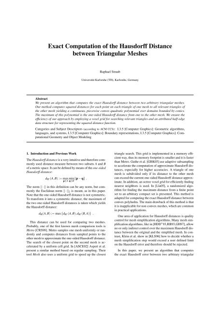
subdivide <strong>the</strong> plane <strong>of</strong> T ′ into seven regions, where each region<br />
contains ei<strong>the</strong>r <strong>the</strong> points p closest to <strong>the</strong> interior <strong>of</strong> T<br />
or closest to one <strong>of</strong> <strong>the</strong> edges or one <strong>of</strong> <strong>the</strong> corners <strong>of</strong> T , see<br />
Fig. 1. These regions are <strong>the</strong> Voronoi regions <strong>of</strong> T , its edges,<br />
and its corners, restricted to <strong>the</strong> plane <strong>of</strong> T ′ . They may be<br />
empty and are obtained by projecting T and six half-lines<br />
emanating from <strong>the</strong> three corners orthogonally to one <strong>of</strong> <strong>the</strong><br />
two adjacent edges into <strong>the</strong> plane <strong>of</strong> T ′ , where <strong>the</strong> projection<br />
direction is orthogonal to T .<br />
Clearly, d 2 T is a continuous function that is quadratic over<br />
each <strong>of</strong> <strong>the</strong>se seven regions:<br />
d 2 ⎧ 2 det[p − a b − a c − a]<br />
if p ∈ Rabc<br />
(b − a) × (c − a)<br />
2 ⎪⎨<br />
(p − a) × (b − a)<br />
if p ∈ Rab<br />
T (p) =<br />
b − a<br />
.<br />
p − a<br />
⎪⎩<br />
2<br />
.<br />
if p ∈ Ra<br />
.<br />
The quadratic functions d 2 T consists <strong>of</strong> are non-negative and<br />
a − b<br />
Ra<br />
T ′<br />
Rab<br />
Rac<br />
a<br />
Rabc<br />
Rbc<br />
Figure 1: The triangle T is projected perpendicularly to T<br />
into <strong>the</strong> plane <strong>of</strong> T ′ dividing it into seven distinct regions<br />
Rabc, Rab, Rbc, Rac, Ra, Rb, and Rc. The boundaries <strong>of</strong> <strong>the</strong><br />
regions Ra, Rb, and Rc lie on planes through <strong>the</strong> corners<br />
<strong>of</strong> T each perpendicular to one <strong>of</strong> <strong>the</strong> two adjacent edges<br />
<strong>of</strong> T . For example, <strong>the</strong> boundary <strong>between</strong> Ra and Rab lies on<br />
<strong>the</strong> plane through a perpendicular to a − b.<br />
<strong>the</strong>refore <strong>the</strong>y are convex, since non-negative quadratic functions<br />
are ei<strong>the</strong>r constant or represent convex parabolic cylinders<br />
or elliptic paraboloids. All o<strong>the</strong>r types <strong>of</strong> quadrics do<br />
not represent functions at all or only functions with negative<br />
values.<br />
Now, to obtain d 2 (cf. Equ. (1)) we have to compute <strong>the</strong><br />
minimum <strong>of</strong> <strong>the</strong> d 2 Ti (i = 1,...,n) over T ′ . The minimum <strong>of</strong><br />
two functions d 2 Ti and d2 Tj is piecewise quadratic, where <strong>the</strong><br />
domains <strong>of</strong> <strong>the</strong> quadratic pieces are bounded by <strong>the</strong> boundaries<br />
<strong>of</strong> <strong>the</strong> regions shown in Fig. 1 and <strong>the</strong> conics given by<br />
<strong>the</strong> equation<br />
Rc<br />
Rb<br />
d 2 Ti (p) = d2 Tj (p) or d2 Ti (p) − d2 Tj (p) = 0 .<br />
These domains are <strong>the</strong> intersections <strong>of</strong> <strong>the</strong> Voronoi regions<br />
<strong>of</strong> all triangles, edges, and vertices <strong>of</strong> M (cf. [Mil93])<br />
with T ′ . Since a convex function reaches its maximum at<br />
<strong>the</strong> boundary <strong>of</strong> its domain, <strong>the</strong> squared distance function<br />
d 2 = min n i=1 d2 Ti has its maximum on one <strong>of</strong> <strong>the</strong>se conics or<br />
line segments. Figure 2 shows <strong>the</strong> graph <strong>of</strong> a squared distance<br />
function for two triangles.<br />
Once <strong>the</strong> maximum <strong>of</strong> d 2 on <strong>the</strong> boundaries <strong>of</strong> its domains<br />
is computed, <strong>the</strong> maximum <strong>of</strong> <strong>the</strong>se values for all triangles<br />
T ′<br />
1 ,...,T ′ m is <strong>the</strong> one-sided <strong>Hausdorff</strong> distance dH ′(M′ ,M).<br />
Algorithm 1 gives a basic overview <strong>of</strong> <strong>the</strong> complete algorithm<br />
for <strong>the</strong> one-sided <strong>Hausdorff</strong> distance. Finally, to obtain<br />
<strong>the</strong> wanted <strong>Hausdorff</strong> distance, <strong>the</strong> o<strong>the</strong>r one-sided <strong>Hausdorff</strong><br />
distance dH ′(M,M′ ) can be determined analogously.<br />
c<br />
T<br />
b
T ′<br />
T1<br />
R. Straub / <strong>Exact</strong> <strong>Computation</strong> <strong>of</strong> <strong>the</strong> <strong>Hausdorff</strong> <strong>Distance</strong> <strong>between</strong> Triangular Meshes<br />
d 2 (p)<br />
Figure 2: The graph <strong>of</strong> <strong>the</strong> piecewise quadratic squared distance<br />
d 2 to two triangles T1 and T2 over a triangle T ′ . The<br />
red and yellow parts <strong>of</strong> <strong>the</strong> graph belong to <strong>the</strong> points that<br />
are nearest to T1 and T2, respectively. The projections <strong>of</strong> T1<br />
and T2 into <strong>the</strong> plane <strong>of</strong> T ′ are depicted in gray.<br />
Algorithm 1 <strong>Computation</strong> <strong>of</strong> <strong>the</strong> one-sided <strong>Hausdorff</strong> dis-<br />
′<br />
tance dH ′({T 1 ,...,T ′ m},{T1,...,Tn})<br />
1: d 2 H ′ := 0<br />
2: for all T ′ ∈ {T ′<br />
1 ,...,T ′ m} do<br />
3: d 2 := ∞<br />
4: for all T ∈ {T1,...,Tn} do<br />
5: compute d 2 T by projecting T into T ′<br />
6: d 2 := min{d 2 ,d 2 T }<br />
7: end for<br />
8: d 2 H ′ := max<br />
9: end for <br />
10: return d2 H ′<br />
3. The Algorithm in Detail<br />
<br />
d 2 H ′, max<br />
p∈T ′ d2 <br />
(p)<br />
In this section, we explain how our one-sided <strong>Hausdorff</strong> distance<br />
computation can be implemented. Especially, we go<br />
into <strong>the</strong> details <strong>of</strong> <strong>the</strong> squared distance function computation<br />
and <strong>the</strong> selection <strong>of</strong> relevant triangles.<br />
3.1. Computing <strong>the</strong> Squared <strong>Distance</strong> Function<br />
We store <strong>the</strong> squared distance functions d 2 in a half-edge<br />
data structure (cf. [BSBK02]), which is commonly used for<br />
meshes. Here, <strong>the</strong> edges <strong>of</strong> <strong>the</strong> mesh represent <strong>the</strong> conic<br />
boundaries <strong>of</strong> <strong>the</strong> domains and <strong>the</strong> faces represent <strong>the</strong> domains.<br />
Hence, <strong>the</strong> edges have <strong>the</strong> equation <strong>of</strong> <strong>the</strong> boundary<br />
conic and <strong>the</strong> faces <strong>the</strong> equation <strong>of</strong> d 2 in <strong>the</strong> corresponding<br />
domain as attributes. This attributed mesh data structure<br />
enables us to split and merge faces and to find adjacent domains<br />
in constant time.<br />
The squared distance function d 2 over a triangle T ′ is<br />
p<br />
T2<br />
<strong>the</strong> minimum over all squared distance functions d 2 T (T ∈<br />
{T1,...,Tn}). As this minimum is computed incrementally<br />
over all relevant triangles T (cf. line 6 in Algorithm 1), we<br />
assume in <strong>the</strong> following that we already have a squared distance<br />
function d 2 in our attributed mesh data structure. Our<br />
goal is now to insert <strong>the</strong> distance function d 2 T <strong>of</strong> a new triangle<br />
T into our data structure so that it represents <strong>the</strong> minimum<br />
<strong>of</strong> d 2 and d 2 T .<br />
The projection <strong>of</strong> T into T ′ divides <strong>the</strong> attributed mesh<br />
into at most seven regions (cf. Fig. 1). For each domain, d 2 is<br />
compared to <strong>the</strong> new distance function d 2 T for all overlapping<br />
regions by computing <strong>the</strong> conic Q(p) := d 2 (p)−d 2 T (p) = 0.<br />
This conic is <strong>the</strong>n trimmed by <strong>the</strong> boundaries <strong>of</strong> <strong>the</strong> domain<br />
and <strong>the</strong> corresponding region. The remaining part <strong>of</strong><br />
<strong>the</strong> conic, if existent, yields a new edge and <strong>the</strong> region <strong>of</strong><br />
all p where Q(p) > 0, i. e., d 2 T (p) < d 2 (p), yields a new face<br />
in <strong>the</strong> domain mesh. Potential resulting adjacent faces where<br />
d 2 is <strong>the</strong> same polynomial can be merged subsequently.<br />
As <strong>the</strong> global maximum <strong>of</strong> <strong>the</strong> squared distance function<br />
d 2 over T ′ is achieved on <strong>the</strong> boundary <strong>of</strong> a domain, this<br />
maximum is <strong>the</strong> maximum <strong>of</strong> all local maxima on <strong>the</strong> edges<br />
and <strong>the</strong> values <strong>of</strong> d 2 at <strong>the</strong> vertices <strong>of</strong> <strong>the</strong> domain mesh. To<br />
determine <strong>the</strong> local maxima on <strong>the</strong> edges we parameterize d 2<br />
over each <strong>of</strong> its boundary conics Q(p) = 0 by using a rational<br />
quadratic parameterization f : R → R 3 , Q(f(t)) = 0 (t ∈ R)<br />
<strong>of</strong> Q (cf. [Far95, pp. 61f]). The resulting parameterization<br />
d 2 (t) := d 2 (f(t)) is a rational quartic polynomial in t whose<br />
local maxima can be computed in a straightforward manner.<br />
3.2. Selecting Relevant Triangles<br />
Our main algorithm consists <strong>of</strong> two nested loops (cf. lines 2<br />
and 4 in Algorithm 1) over all triangles <strong>of</strong> <strong>the</strong> meshes M ′<br />
and M. We should avoid computing <strong>the</strong> squared distance<br />
functions d 2 for all pairs <strong>of</strong> triangles <strong>of</strong> M ′ and M as <strong>the</strong><br />
number <strong>of</strong> triangles in each mesh can exceed some millions<br />
and <strong>the</strong> computation <strong>of</strong> d 2 will become time-consuming.<br />
Since for each triangle T ′ ⊆ M ′ we are only interested<br />
in <strong>the</strong> distance to <strong>the</strong> nearest triangles T ⊆ M, we start projecting<br />
near triangles into T ′ and stop as soon as we are sure<br />
that all o<strong>the</strong>r triangles <strong>of</strong> M are too far away to change d 2 . To<br />
speed up this process we use a voxel grid as a spatial search<br />
structure. In a preprocessing step all triangles <strong>of</strong> M and M ′<br />
are inserted into all voxels <strong>the</strong>y intersect, where each voxel<br />
has two lists, one for <strong>the</strong> triangles <strong>of</strong> each <strong>of</strong> <strong>the</strong> two meshes.<br />
The size <strong>of</strong> <strong>the</strong> voxel grid is determined by <strong>the</strong> size l ×<br />
w × h <strong>of</strong> <strong>the</strong> bounding box <strong>of</strong> M ∪ M ′ and <strong>the</strong> number n +<br />
m <strong>of</strong> triangles. Assuming that <strong>the</strong> voxels are approximately<br />
cubical with edge length a and that all triangles have <strong>the</strong><br />
same size and are equally distributed on <strong>the</strong> surface <strong>of</strong> <strong>the</strong><br />
bounding box, we have<br />
k =<br />
a2 (n + m)<br />
2(lw + lh + wh)
R. Straub / <strong>Exact</strong> <strong>Computation</strong> <strong>of</strong> <strong>the</strong> <strong>Hausdorff</strong> <strong>Distance</strong> <strong>between</strong> Triangular Meshes<br />
triangles per voxel. In practice, we select, e. g., k = 1 and<br />
compute <strong>the</strong> corresponding approximate size a <strong>of</strong> <strong>the</strong> voxels<br />
through <strong>the</strong> equation above.<br />
The selection <strong>of</strong> relevant triangles T for which to compute<br />
<strong>the</strong> squared distance function d 2 T starts with one triangle<br />
<strong>of</strong> M in <strong>the</strong> voxel nearest to one voxel <strong>of</strong> T ′ . The nearest<br />
voxel is found using a breadth-first search strategy starting<br />
with <strong>the</strong> voxels <strong>of</strong> T ′ . In each iterative step, after <strong>the</strong> update<br />
<strong>of</strong> <strong>the</strong> squared distance function d 2 (cf. line 6 in Algorithm 1)<br />
<strong>the</strong> maximum dmax := maxp∈T ′ d2 (p) is computed. For all<br />
following steps only triangles T in voxels that have at least<br />
one point nearer than dmax to a point in a voxel <strong>of</strong> T ′ are<br />
considered. All o<strong>the</strong>r triangles are far<strong>the</strong>r than dmax away<br />
from T ′ , so <strong>the</strong>y do not contribute to <strong>the</strong> minimum <strong>of</strong> all d 2 Ti .<br />
4. Conclusion and Future Work<br />
The algorithm presented in this paper computes <strong>the</strong> exact<br />
<strong>Hausdorff</strong> distance <strong>between</strong> triangular meshes. An implementation<br />
and subsequent tests on real world examples are<br />
planned for <strong>the</strong> future. It is obvious that our method can<br />
be easily employed for arbitrary piecewise linear surfaces,<br />
as it does not make use <strong>of</strong> <strong>the</strong> mesh connectivity and nontriangular<br />
meshes can be triangulated before. A straightforward<br />
extension <strong>of</strong> our method would be to compute <strong>the</strong> mean<br />
squared distance by taking <strong>the</strong> integral <strong>of</strong> <strong>the</strong> squared distance<br />
function over a triangle divided by its area.<br />
5. Acknowledgments<br />
We would like to thank Raphael Diziol for creating <strong>the</strong> visualization<br />
<strong>of</strong> <strong>the</strong> squared distance function and Bertrand<br />
Klimmek for pro<strong>of</strong>-reading this paper.<br />
References<br />
[ASCE02] ASPERT N., SANTA-CRUZ D., EBRAHIMI T.:<br />
Mesh: Measuring errors <strong>between</strong> surfaces using <strong>the</strong> <strong>Hausdorff</strong><br />
distance. In Proceedings <strong>of</strong> <strong>the</strong> IEEE International<br />
Conference on Multimedia and Expo (ICME) (2002),<br />
vol. 1, pp. 705–708.<br />
[BSBK02] BOTSCH M., STEINBERG S., BISCHOFF S.,<br />
KOBBELT L.: Openmesh – a generic and efficient polygon<br />
mesh data structure. In OpenSG Symposium (2002).<br />
[CRS98] CIGNONI P., ROCCHINI C., SCOPIGNO R.:<br />
Metro: Measuring error on simplified surfaces. Computer<br />
Graphics Forum 17, 2 (1998), 167–174.<br />
[Far95] FARIN G. E.: NURB Curves and Surfaces. A K<br />
Peters, Wellesley, MA, 1995.<br />
[GBK05] GUTHE M., BORODIN P., KLEIN R.: Fast and<br />
accurate <strong>Hausdorff</strong> distance calculation <strong>between</strong> meshes.<br />
In Proceedings <strong>of</strong> <strong>the</strong> 13th International Conference in<br />
Central Europe on Computer Graphics, Visualization and<br />
Computer Vision (WSCG) (2005), pp. 41–48.<br />
[GH97] GARLAND M., HECKBERT P. S.: Surface simplification<br />
using quadric error metrics. In Proceedings <strong>of</strong> <strong>the</strong><br />
24th annual conference on Computer graphics and interactive<br />
techniques (1997), pp. 209–216.<br />
[HDD ∗ 93] HOPPE H., DEROSE T., DUCHAMP T., MC-<br />
DONALD J., STUETZLE W.: Mesh optimization. Computer<br />
Graphics 27 (1993), 19–26.<br />
[KLS96] KLEIN R., LIEBICH G., STRASSER W.: Mesh<br />
reduction with error control. In IEEE Visualization ’96<br />
(1996), Yagel R., Nielson G. M., (Eds.), pp. 311–318.<br />
[Lla05] LLANAS B.: Efficient computation <strong>of</strong> <strong>the</strong> <strong>Hausdorff</strong><br />
distance <strong>between</strong> polytopes by exterior random covering.<br />
<strong>Computation</strong>al Optimization and Applications 30,<br />
2 (2005), 161–194.<br />
[Mil93] MILENKOVIC V.: Robust construction <strong>of</strong> <strong>the</strong><br />
Voronoi diagram <strong>of</strong> a polyhedron. In Proceedings <strong>of</strong> <strong>the</strong><br />
Fifth Canadian Conference on <strong>Computation</strong>al Geometry<br />
(Aug. 1993), Lubiw A., Urrutia J., (Eds.), pp. 473–478.<br />
[RB93] ROSSIGNAC J. R., BORREL P.: Multi-resolution<br />
3d approximations for rendering complex scenes. In Geometric<br />
Modeling in Computer Graphics (1993), Falcidieno<br />
B., Kunii T. L., (Eds.), Springer Verlag, pp. 455–<br />
465.