Unrestricted and complete Breadth-First Search of trapezoid graphs ...
Unrestricted and complete Breadth-First Search of trapezoid graphs ...
Unrestricted and complete Breadth-First Search of trapezoid graphs ...

Create successful ePaper yourself
Turn your PDF publications into a flip-book with our unique Google optimized e-Paper software.
lirmm-00469844, version 1 - 2 Apr 2010<br />
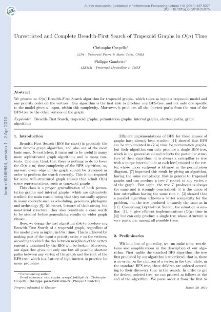
<strong>Unrestricted</strong> <strong>and</strong> Complete <strong>Breadth</strong>-<strong>First</strong> <strong>Search</strong> <strong>of</strong> Trapezoid Graphs in O(n) Time<br />
Abstract<br />
Christophe Crespelle ∗<br />
LIP6 - Université Pierre & Marie Curie, CNRS<br />
Philippe Gambette ∗<br />
LIRMM - Université Montpellier 2, CNRS<br />
We present an O(n) <strong>Breadth</strong>-<strong>First</strong> <strong>Search</strong> algorithm for <strong>trapezoid</strong> <strong>graphs</strong>, which takes as input a <strong>trapezoid</strong> model <strong>and</strong><br />
any priority order on the vertices. Our algorithm is the first able to produce any BFS-tree, <strong>and</strong> not only one specific<br />
to the model given as input, within this complexity. Moreover, it produces all the shortest paths from the root <strong>of</strong> the<br />
BFS-tree to the other vertices <strong>of</strong> the graph.<br />
Keywords: <strong>Breadth</strong>-<strong>First</strong> <strong>Search</strong>, <strong>trapezoid</strong> <strong>graphs</strong>, permutation <strong>graphs</strong>, interval <strong>graphs</strong>, shortest paths, graph<br />
algorithms<br />
1. Introduction<br />
<strong>Breadth</strong>-<strong>First</strong> <strong>Search</strong> (BFS for short) is probably the<br />
most famous graph algorithm, <strong>and</strong> also one <strong>of</strong> the most<br />
basic ones. Nevertheless, it turns out to be useful in many<br />
more sophisticated graph algorithms <strong>and</strong> in many contexts.<br />
One may think that there is nothing to do to lower<br />
the O(n + m) time complexity <strong>of</strong> the BFS algorithm, as,<br />
anyway, every edge <strong>of</strong> the graph should be traversed in<br />
order to perform the search correctly. This is not required<br />
for some well-structured graph classes that admit O(n)<br />
space representations, such as <strong>trapezoid</strong> <strong>graphs</strong>.<br />
This class is a proper generalization <strong>of</strong> both permutation<br />
<strong>graphs</strong> <strong>and</strong> interval <strong>graphs</strong>, which are extensively<br />
studied; the main reason being that they naturally appear<br />
in many contexts such as scheduling, genomics, phylogeny<br />
<strong>and</strong> archeology [6]. Moreover, because <strong>of</strong> their strong but<br />
non-trivial structure, they also constitute a case worth<br />
to be studied before generalizing results to wider graph<br />
classes.<br />
Here, we design the first algorithm able to produce any<br />
<strong>Breadth</strong>-<strong>First</strong> <strong>Search</strong> <strong>of</strong> a <strong>trapezoid</strong> graph, regardless <strong>of</strong><br />
the model given as input, in O(n) time. This is achieved by<br />
making part <strong>of</strong> the input a priority order σ on the vertices,<br />
according to which the ties between neighbors <strong>of</strong> the vertex<br />
currently examined by the BFS will be broken. Moreover,<br />
our algorithm gives not only one but all possible shortest<br />
paths between any vertex <strong>of</strong> the graph <strong>and</strong> the root <strong>of</strong> the<br />
BFS-tree, which is a feature <strong>of</strong> high interest in practice for<br />
many problems.<br />
∗ Corresponding author<br />
Email addresses: christophe.crespelle@lip6.fr (Christophe<br />
Crespelle), philippe.gambette@lirmm.fr (Philippe Gambette)<br />
Author manuscript, published in "Information Processing Letters 110 (2010) 497-502"<br />
DOI : 10.1016/j.ipl.2010.03.015<br />
Efficient implementations <strong>of</strong> BFS for these classes <strong>of</strong><br />
<strong>graphs</strong> have already been studied: [11] showed that BFS<br />
can be implemented in O(n) time for permutation <strong>graphs</strong>,<br />
but their algorithm can only produce a single BFS-tree,<br />
which is not general at all <strong>and</strong> reflects the particular structure<br />
<strong>of</strong> their algorithm: it is always a caterpillar (a tree<br />
with a unique internal node at each level) rooted at the vertex<br />
whose upper endpoint is leftmost in the permutation<br />
diagram. [7] improved this result by giving an algorithm,<br />
having the same complexity, that is general to <strong>trapezoid</strong><br />
<strong>graphs</strong> <strong>and</strong> can produce a tree T rooted at any vertex r<br />
<strong>of</strong> the graph. But again, the tree T produced is always<br />
the same <strong>and</strong> is strongly constrained: it is the union <strong>of</strong><br />
four caterpillars having the same root r. [3] showed that<br />
a parallel algorithm achieves a better complexity for the<br />
problem, but the tree produced is exactly the same as in<br />
[11]. Concerning Depth-<strong>First</strong> <strong>Search</strong>, the situation is similar:<br />
[11, 4] give efficient implementations (O(n) time in<br />
[4]) but can only produce a single tree whose structure is<br />
very particular among all possible trees.<br />
2. Preliminaries<br />
Without loss <strong>of</strong> generality, we can make some restrictions<br />
<strong>and</strong> simplifications in the description <strong>of</strong> our algorithm.<br />
<strong>First</strong>, unlike the st<strong>and</strong>ard BFS algorithm, the tree<br />
first produced by our algorithm is unordered, that is, there<br />
is no order on the children <strong>of</strong> a vertex in the tree, while, in<br />
the st<strong>and</strong>ard BFS-tree, these children are ordered according<br />
to their discovery time in the search. In order to get<br />
the desired ordered tree, we can proceed as follows at the<br />
end <strong>of</strong> the algorithm. We parse order σ from the first to<br />
Preprint submitted to Elsevier March 29, 2010
lirmm-00469844, version 1 - 2 Apr 2010<br />
the last vertex, <strong>and</strong> for each vertex, we remove it from the<br />
list <strong>of</strong> children <strong>of</strong> its father <strong>and</strong> insert it again at the end<br />
<strong>of</strong> this list. This takes O(n) time <strong>and</strong> orders the lists <strong>of</strong><br />
children with regard to σ, as desired. As a consequence,<br />
in the following, we only consider the construction <strong>of</strong> the<br />
unordered tree.<br />
In addition, we focus on the case where the input graph<br />
is connected. If it is not, our algorithm performs the BFS<br />
<strong>of</strong> the connected component <strong>of</strong> the first vertex in σ, without<br />
any modification <strong>of</strong> its description. Then, the algorithm<br />
can go on starting from the first non-visited vertex<br />
<strong>of</strong> σ. Finding this vertex can be done in constant time<br />
by maintaining along the algorithm the list <strong>of</strong> non-visited<br />
vertices, ordered with regard to σ.<br />
Definitions <strong>and</strong> Notations. All <strong>graphs</strong> considered here are<br />
finite, undirected, loopless <strong>and</strong> simple. V is the vertex<br />
set <strong>of</strong> graph G <strong>and</strong> E is its edge set, which we denote by<br />
G = (V, E). Throughout the paper, n st<strong>and</strong>s for |V |. An<br />
edge between vertices x <strong>and</strong> y will be arbitrarily denoted<br />
xy or yx. The neighborhood <strong>of</strong> x is denoted N(x). T<br />
denotes the BFS-tree to be produced. The depth <strong>of</strong> node<br />
u in T is its distance from the root. The set <strong>of</strong> vertices at<br />
depth i in T will be denoted T i (T 0 contains only the root<br />
<strong>of</strong> T ). For a linear ordering σ on a set S, we denote min(σ)<br />
(resp. max(σ)) for the first (resp. last) element <strong>of</strong> σ. For<br />
s ∈ S, s − (resp. s + ) denotes for the predecessor (resp.<br />
successor) <strong>of</strong> s in σ. The interval <strong>of</strong> σ made <strong>of</strong> vertices<br />
between a <strong>and</strong> b, with a ≤σ b, is denoted a, b. The list L<br />
containing elements x1, . . . , xk is denoted L = [x1, . . . , xk].<br />
The concatenation <strong>of</strong> two lists L1, L2 is denoted L1.L2.<br />
A <strong>trapezoid</strong> model <strong>of</strong> a graph G is a set <strong>of</strong> <strong>trapezoid</strong>s<br />
between two horizontal lines (two endpoints on the upper<br />
line <strong>and</strong> two endpoints on the lower line) together with<br />
a one to one mapping onto the set <strong>of</strong> vertices <strong>of</strong> G, such<br />
that there is an edge between vertices x <strong>and</strong> y in G iff their<br />
corresponding <strong>trapezoid</strong>s intersect. A <strong>trapezoid</strong> graph is<br />
a graph admitting such a model. Note that a <strong>trapezoid</strong><br />
model can be computed from the graph in time O(n 2 ) using<br />
the algorithm <strong>of</strong> [9]. The class remains the same if<br />
the <strong>trapezoid</strong>s are required to be closed <strong>and</strong> to have distinct<br />
integer endpoints between 1 <strong>and</strong> 2n on both lines.<br />
All models considered here satisfy this restriction. More<br />
precisely, in the following, a <strong>trapezoid</strong> model will be considered<br />
as a couple (π1, π2) <strong>of</strong> orders on some subsets <strong>of</strong><br />
<strong>trapezoid</strong> endpoints <strong>of</strong> the model: π1 is the left to right<br />
order <strong>of</strong> the endpoints on the upper line, <strong>and</strong> π2 is the left<br />
to right order <strong>of</strong> the endpoints on the bottom line. Each<br />
vertex v is associated with the four endpoints <strong>of</strong> its corresponding<br />
<strong>trapezoid</strong>, which are denoted v l 1, v r 1, v l 2 <strong>and</strong> v r 2 for<br />
the top-left, top-right, bottom-left <strong>and</strong> bottom-right endpoint<br />
respectively. This provides an efficient encoding <strong>of</strong><br />
the graph that takes O(n) space <strong>and</strong> allows to answer adjacency<br />
queries between any pair <strong>of</strong> vertices in O(1) time. In<br />
the sequel, we <strong>of</strong>ten identify vertices <strong>and</strong> their associated<br />
<strong>trapezoid</strong>s.<br />
2<br />
BuildTree(π1, π2, σ)<br />
1. x ← min(σ); ord(x) ← 1; color x in gray<br />
2. initialize I <strong>and</strong> Γ with (x l 1, x r 1, x l 2, x r 2)<br />
3. For all y ∈ N(x) Do<br />
4. parent(y) ← x; color y in gray; update(Γ, y)<br />
5. While I = Γ Do<br />
6. Γnew ← Γ; Ex ← ∅<br />
7. If α l 1 π1 b r 1 Then PutInTree(β r 1, b r+<br />
1 , π1, r, Qr 9.<br />
1)<br />
If γ l 2 π2 d r 2 Then PutInTree(δ r 2, d r+<br />
2 , π2, r, Qr 11.<br />
2)<br />
AssignOrd(Q l 1, Q r 1, Q l 2, Q r 2); color Ex in gray<br />
12. I ← Γ; Γ ← Γnew<br />
Figure 1: Routine BuildTree. Lists Ql 1 , Qr 1 , Ql 2 , Qr 2 <strong>and</strong> Ex are<br />
global variables, as well as I = (al 1 , br 1 , cl 2 , dr 2 ), Γ = (αl 1 , βr 1 , γl 2 , δr 2 )<br />
<strong>and</strong> Γnew which contain quadruplets <strong>of</strong> endpoints.<br />
PutInTree(u side<br />
k , v t k, πk, side, Q)<br />
1. p ← u; Q ← [p]<br />
2. For y s k from u side<br />
k<br />
to v t k in πk Do<br />
3. If y white & s = side & p
lirmm-00469844, version 1 - 2 Apr 2010<br />
<br />
0≤j≤i T j , <strong>and</strong> I1 is the interval containing the upper endpoints<br />
<strong>of</strong> the vertices <strong>of</strong> <br />
0≤j≤i−1 T j ; intervals Γ2 <strong>and</strong> I2<br />
are similarly defined in π2 for lower endpoints.<br />
Each level <strong>of</strong> the tree is built by parsing the endpoints<br />
in Γ1\I1 <strong>and</strong> Γ2\I2, which are split in four intervals, thanks<br />
to the four calls to Routine PutInTree (Lines 7 to 10 <strong>of</strong><br />
BuildTree). The new vertices encountered during this<br />
parse are exactly those <strong>of</strong> T i+1 , which are then assigned<br />
their parent in T . It is important to note that our algorithm<br />
does not discover the vertices in the same order as<br />
the st<strong>and</strong>ard BFS would do. Despite <strong>of</strong> this, we are able<br />
to determine, for each vertex, its correct parent in the<br />
BFS-tree, thanks to function ord. ord numbers a subset<br />
<strong>of</strong> vertices in each level <strong>of</strong> the tree computed so far, except<br />
in the last one T i . Its essential property is that, at the<br />
beginning <strong>of</strong> the ith iteration <strong>of</strong> the main loop, every vertex<br />
<strong>of</strong> level T i−1 having children in T is numbered <strong>and</strong> the<br />
order induced by ord on these vertices is exactly the order<br />
in which the st<strong>and</strong>ard BFS discovers them. Together with<br />
order σ, it allows to determine the parent <strong>of</strong> the vertices<br />
<strong>of</strong> level T i+1 <strong>and</strong> to assign their ord value to vertices <strong>of</strong><br />
T i (at least to those having children in T ). Note that a<br />
vertex may be assigned a parent twice by our algorithm:<br />
in this case, the second one is the correct one.<br />
Before the algorithm starts, for every vertex y, parent(y)<br />
is initialized with ⊥, <strong>and</strong> y is colored white. During the<br />
algorithm, vertices are colored gray once they have been<br />
assigned their correct parent in the tree. This is done at<br />
the end <strong>of</strong> the main loop <strong>of</strong> Routine BuildTree (Line 11).<br />
We denote by (al 1, br 1) (resp. (αl 1, βr 1), (cl 2, dr 2), (γl 2, δr 2)) the<br />
left <strong>and</strong> right endpoint <strong>of</strong> I1 (resp. Γ1, I2, Γ2). Remark<br />
that this notation is coherent, since it is a straightforward<br />
property <strong>of</strong> our algorithm that the left (resp. right) endpoint<br />
<strong>of</strong> any <strong>of</strong> these four intervals is always the left (resp.<br />
right) endpoint <strong>of</strong> some <strong>trapezoid</strong> <strong>of</strong> the model. For y ∈ V<br />
<strong>and</strong> a quadruplet X = (l1, r1, l2, r2) <strong>of</strong> endpoints such<br />
that l1, r1 ∈ π1 <strong>and</strong> l2, r2 ∈ π2, procedure update(X, y)<br />
executes the instructions lj ← minπj (lj, y l j ) <strong>and</strong> rj ←<br />
maxπj (rj, yr j ), for j ∈ {1, 2}. Function ord takes integer<br />
values which are assigned by Procedure AssignOrd.<br />
Order
lirmm-00469844, version 1 - 2 Apr 2010<br />
similar. Since y is white, y ∈ T i <strong>and</strong> therefore is not adjacent<br />
to any vertex <strong>of</strong> T i−1 , which implies that y l 1 >π1 br 1<br />
<strong>and</strong> y l 2 >π2 dr 2. Moreover, since b r 1 = β r 1, Property 1 <strong>and</strong> 2<br />
<strong>of</strong> the invariant ensures that β ∈ T i . If i = 1, from Property<br />
3 <strong>of</strong> the invariant, β has at least one endpoint in I1∪I2.<br />
It follows that β l 1
lirmm-00469844, version 1 - 2 Apr 2010<br />
Invariant 2. For any i ≥ 1, at the beginning <strong>of</strong> the i th<br />
iteration <strong>of</strong> the main loop, the subset O i−1 <strong>of</strong> vertices <strong>of</strong><br />
T i−1 for which ord is defined contains all the vertices <strong>of</strong><br />
T i−1 that have children in T . And the order induced by<br />
ord on vertices <strong>of</strong> O i−1 is exactly the order <strong>of</strong> visit <strong>of</strong> those<br />
vertices by the st<strong>and</strong>ard BFS algorithm.<br />
Pro<strong>of</strong>. Since ord(x) is initialized to 1 at Line 1 <strong>of</strong> Routine<br />
BuildTree, the invariant clearly holds for i = 1. Suppose<br />
it holds for some i ≥ 1. Then, since ord is defined for<br />
every parent <strong>of</strong> the vertices <strong>of</strong> T i , order
lirmm-00469844, version 1 - 2 Apr 2010<br />
most) two pointers. The total size <strong>of</strong> the four lists assigned<br />
to level T i is dominated by the number <strong>of</strong> vertices in T i−1 .<br />
Thus the size <strong>of</strong> the additional space needed to store the<br />
whole data structure is O(n).<br />
In practice, it may be desirable to follow the shortest<br />
paths in the other way: from the root <strong>of</strong> T to the other<br />
vertices <strong>of</strong> G. To this purpose one must store, for each vertex<br />
at level i, its set <strong>of</strong> neighbors at level i+1. This can be<br />
done very similarly to what precedes. During the i th iteration<br />
<strong>of</strong> the loop, for each execution <strong>of</strong> PutInTree, build<br />
the list <strong>of</strong> white vertices encountered by pushing them on<br />
a stack. When a gray vertex z is encountered, assign to<br />
it a pointer to the top <strong>of</strong> the stack: the neighbors <strong>of</strong> z at<br />
level i+1 are the white vertices that are above this pointer<br />
in the stack (Lemma 2).<br />
3.4. Complexity<br />
<strong>First</strong> <strong>of</strong> all, note that the computation <strong>of</strong> the lists storing<br />
all shortest paths from nodes <strong>of</strong> the <strong>graphs</strong> to the root<br />
x <strong>of</strong> T only requires constant additive extra-time in the<br />
treatment <strong>of</strong> an endpoint. This does not change the overall<br />
complexity <strong>of</strong> the algorithm <strong>and</strong>, for sake <strong>of</strong> simplicity,<br />
we do not take it into account anymore in the complexity<br />
analysis.<br />
The complexity <strong>of</strong> Routine BuildTree is O(n). Let B<br />
denote (Γ1 \ I1) ∪ (Γ2 \ I2). At Line 3, we can get N(x) in<br />
O(n) time, by scanning π1 <strong>and</strong> π2, <strong>and</strong> the running time <strong>of</strong><br />
the initialization loop (Lines 3 <strong>and</strong> 4) is O(|N(x)|) = O(n).<br />
In Routine PutInTree(uside k , vt k , πk, side, Q), all instructions<br />
take O(1) time, <strong>and</strong> the routine runs in O(|uside k , vt k|) time. This gives an O(|B|) time bound for the four calls<br />
<strong>of</strong> Lines 7 to 10 <strong>of</strong> BuildTree. Coloring list Ex also takes<br />
O(|B|) time. The complexity <strong>of</strong> procedure AssignOrd<br />
is a crucial point. It is important to note that any list<br />
Q ′ ∈ {Ql 1, Qr 1, Ql 2, Qr 2} being one <strong>of</strong> its arguments is already<br />
sorted according to order