A summary of Modeling and Simulation

A summary of
Modeling and Simulation
Text-book: Modeling of dynamic
systems
– Lennart Ljung and Torkel Glad

Content
• What’re Models for systems and signals?
– Basic concepts
– Types of models
• How to build a model for a given system?
– Physical modeling
– Experimental modeling
• How to simulate a system? y
– Matlab/Simulink tools
• CCase studies
t di

SSystems stems and models
• Part one – Models, p13-78
• SSystem t iis ddefined fi d as an object bj t or a collection ll ti of f
objects whose properties we want to study
• A model of a system is a tool we use to answer
questions about the system without having to do
an experiment
– MMental t l model d l
– Verbal model
– Physical model
– Mathematical model

HHow tto build b ild and d validate lid t models d l
• Physical modeling: laws of nature
• Experimental modeling: Identification
•Any y models have a limited domain of
validation

TTypes pes of mathematical models
• Deterministic & stochastic
• Dynamic & static
• Continuous time & discrete time
• Lumped p & distributed
• Change oriented & discrete event driven

Models for systems y and signals g
(Chapter 3)
• Block diagram models: logical
decomposition of the functions of the
system y and show how the different
parts(blocks) influence each other
u(t)
h(t)
q(t)
Bernoulli’s law: v(t)=sqrt(2gh(t))
u(t)
q(t)
Tank model (1) h(t)

EExample ample of Flow Flo ddynamic namic
u(t)
h(t)
q(t)
dh() t a 2h 1
=− ht () + ut ()
dt A A
qt () = a 2 ght ()

Parameters & Signals
• Parameters: system parameters & design
parameters t
• Signals (variables):
– external signals: input and disturbance
– Output signals
– Internal variables

Description of ssystems stems
• Differential/difference equations
– High-order DE Transfer functions
• Linearization – equilibrium q p point ( (stationary), y),
Taylor expansion
• Laplace transform/Z transform/Z-transform transform
– First-order DE (define internal variables)
state space models
• Linearization – equilibrium point, Taylor expansion
• State variables

Si Signal l ddescriptions: i ti Ti Time-domain d i
• Deterministic & analytic: u(t)=sin(200t)
• Deterministic & sampled: {u(n)}
• Non Non-deterministic deterministic & analytic: u(t)=
sin(2t)+w(t)
• Non-deterministic & sampled: {u(n)} of
random variable u(t) – stochastic
processes p ( (DE sem6) )

Si Signal l ddescriptions: i ti FFrequency ddomain i
• Concept of frequency – harmonic signals
• High freq. & low freq. Signals
• Fourier transform
•Amplitude p spectrum p
• Power Spectrum of a signal is the sqaure
of the absolute value of its Fourier
transform
• FFT algorithms (DE 6sem)

SSystem t descriptions: d i ti Ti Time-domain d i
Deffierential/differenece equations
• ODE (lumped) & PDE (distributed)
• Linear & nonlinear

Effects of system y to input p signal g

SSystem t descriptions: d i ti ffrequency domain d i
• Laplace transform/Z-transform
• TTransfer f functions f ti for f linear li lumped l d ODE
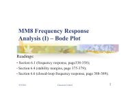
• Bode plot/Nyquist plot

Link between time and frequency q y
domain – systems
• Response to input – Bode plot
• Stability – pole locations
• Performance (overshoot, (overshoot settling time time,
resonance freq.) – pole locations
• Bandwidth
• robustness

Example p Effects of Group p Delay y
The filter has considerable attenuation
at ω=0 ω=0.85π. 85π The group delay at ω=0 ω=0.25π 25π
is about 200 steps, while at ω=0.5π, the
group delay is about 50 steps

CConnection ti of f systems t and d signals i l
• Time-domain: ODE
&& yt () + 2 yt & () + yt () = ut & () + ut ()
yk ( ) − yk ( − 1) + 2 yk ( − 2) = uk ( ) −uk ( −1)
⎧ Xt & () = AXt () + BUt () ⎧ X ( k ) = AX ( k k− 1) +
BU ( k k−
1)
⎨ ⎨
⎩Yt
() = CXt () ⎩Yk
( ) = CXk ( )
• Frequency q y domain: Y () s s+
1
Gs () = = 2
U() s s + 2s+ 1
TF
U(s) G(s) Y(s)
−1
Y( z) 1−z
Gz ( ) = = −1 −2
U( z) 1− z + 2z
−1
Gs () = CsII ( − A) B

Link betwen continuous time and
discrete time models
• Sampling mechanism
• Aliasing problem
• See more from Digital control course course….

Content
• What’re Models for systems and signals?
– Basic concepts
– Types of models
• How to build a model for a given system?
– Physical modeling
– Experimental modeling
• How to simulate a system? y
– Matlab/Simulink tools
• CCase studies
t di

Physical modeling
Part II in textbook pp.79-121

Principle and Phases
• Use the knowledge of physics that is relevant to
the considered system
• Ph Phase 11: structure t t th the problem: bl ddecomposition iti
(cause and effect, variables) block diagram
• Phase 2: formulate subsystems
• Phase 3: get system model via simplification
E l d li th h d b f
• Example: modeling the head box of a paper
machine (pp.85-95)

FFormulation l ti of f physical h i l modeling d li
• Conservation laws
– Mass balance
– Energy balance
– Electronics (Kirchhoff’s laws)
• Constitutive relationships

Simplification of modeling
Principles
• Neglect small effects (approximation)
• Separate time constants
(T_max/T_min

Some relationships in ph physics sics
• Electrical circuits
• Mechanical translation
• Mechanical rotation
• Flow systems y
• Thermal systems
• Lagrange modeling method
• FFor more, see BRP’s BRP’ llectures…. t

Newton’s Newton s 2 2law law
m a = ∑ F
27

Newton’s Newton s 2 law for Rotation
J dω/dt = ∑
τ

DC motor with Permanent Magnet
29

Electro-Mechanical Electro Mechanical Energy Conversion
Chassis or basket
Voice coil
S N
Input Dust cap
Magnet
S N
Suspension
Cone
Force produced by current:
F = Bl I (ved fastholdt svingspole)
F: Kraften på membranen
B: magnetfelt
L: svingspolens trådelængde
I: strømmen
Surround
D t Electro Magnetic force (EMF) and
back EMF
Current produced by membrane
velocity:
emf = Bl v
emf: modelektromotorisk kraft
v: membranens hastighed

U in(t) +
Block Diagram: Loudspeaker
-
+
+ +
1/L e
R e
Bl
∫
v(t)
i(t) F(t)
+
a(t) v(t) x(t)
Bl
1/m ∫ ∫
m
-
+
+ +
r m
1/c m

• Thermal systems, y , Head flow, , modelling g of
geometric problems (for DE5); mm4 2007
DE5 DE5.ppt ppt
• Time and Frequency Response of 1.
and 2. order systems (for M5); mm4 2007
M5 M5.ppt t
• Linearization; mm5 2006 2006.ppt ppt
• Linearization: solution of exercise; mm5
soulution.ppt

Lagrange modeling method
• Generalized coordinate
• Kinetic energy T
• Potential energy V
• External forces along gggerneralized
coordinator Q

Experimental modeling
(nonparametric identification)
Part III in textbook pp.189-223
•Estimation of transient response
•Estimation of transfer function

Estimation of transient response p
(direct method)
• Transient responses:
impulse response, step response
• Arrange experiment (input signal)
• Curve fitting, g, range g scaling, g, time constant
• Transient analysis is easy and most widely
used
• Potential problem: poor accuracy due to
disturbances and measurement errors etc.

Estimation of transient response p
(Correlation analysis)
• Need knowledge of stochastic processes(SEM6)
• Procedure:
– Collect data y(k), u(k), k=1,2,….,N
– Substract sample means from each signal:
N N
1 1
y( k) = y( k) − ∑y( t), u( k) = u( k) − ∑u(
t),
N N
t t= 1 t t=
1
∞
∑
yt () = gut ( − k) + vt ()
– Form signal via whitening filter L(q) (polynomial, lease square):
– Impulse p response: p
y ( k) = L( q) y( k), u ( k) = L( q) u( k)
F F
Rˆ
( τ ) 1 1
g where R y
tu t u t
N N N
N yFuF ˆ N
ˆ
2
ˆ ττ
= y ( ) ( ) ( ), ( )
ˆ
Fu( τ ) =
F ∑ F( ) F( − τ), λN=
∑ F(
)
FuF ∑ F F N ∑
F
λ N t 1 N
N
= t=
1
k = 0
k

Estimation of transient response p
Basic properties:
(Correlation analysis)
• Quick insight into time constants and time delays
• Mo special inputs are required. required
• Poor SNR can be compensated by longer dtata
recordes
• Limitation: input u(t) is uncorrelated with
disturbance v(t). This method won’t work properly
when the dtata are collected from a system under
∞
output feedback y () t = g ut ( − k ) + vt ()
∑
k = 0
∑
k

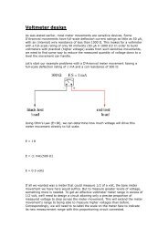
Estimation of transfer functions
(frequency analysis -1)
• Direct frequency analysis (Bode plot)
H(ejω) = |H(ejω)| e

Estimation of transfer functions
• Advantages
(frequency analysis -2)
– Easy to use and requires no complicated data
processing
– RRequires i no strustural t t l assumptions ti other th th than it
being linear
– Easy to concentrate on freq. Ranges of special
interest
• Disadvantages
– Graphic result (Bode plot)
– Need long time of experimentation

Estimation of transfer functions
(Fourier analysis -1)
• Principle: Y( jΩ)
G( jΩ
) =
U ( j Ω )
T( ω) =
N
∑ (
− jωkT ) , T(
ω)
=
N
∑ (
− jωkT )
k= 1 k=
1
Y j T y kT e U j T u kT e
Y YT ( j jω
)
GN( jω)
=
U ( jω)
T
• Evaluation:
T T
− jΩt − jΩt T( Ω ) = ∫ ( ) , ( ) ( )
0
T Ω = ∫0
Y j y t e dt U j u t e dt
ˆ Y YT ( j Ω )
G( jΩ
) =
U ( jΩ)
2 cc u g | V VN ( jjωω
)|
| GN( jω) −G( jω)|
≤ + ,
| UN( jω)| | UN( jω)|
where
system y() t = g( τ) u( t − τ) dτ + v() t
input lim itation : | u( t) | ≤ cu
∫
0
∞
system property : τ | g( τ)| dτ = cg
∫
0
∞
T

Estimation of transfer functions
• Advantages:
(Fourier analysis -2)
– Easy and efficient to use (FFT)
– Good estimation of G(jw) at frequencies
where the input has pure sinusoids
• Di Disadvantages: d t
– The estimation is wildly fluctuating graph,
which only gives a rough picture of the true
frequency domain (see Fig8 Fig8.13, 13 pp pp.209)
209)

Estimation of transfer functions
• Principle:
(Spectra analysis -1)
R ( k) = g( k)* R ( k) R ( k) = g( k)* g( −k)*
R ( k)
yu uu yy uu
Φ ω = ω Φ ω Φ ω = ω Φ ω +Φ ω
2
yu ( ) G( ) uu ( ) yy ( ) | G(
)| uu ( ) vv vv(
)
• Spectra p estimation ( (Black-Tukey’s y spectral p
estimate) - Window function
N
N 1
R Ryu ( k ) = ∑ yt ( + k ) ut ( )
N
t=
1
γ
γ N − jωk Φ yu ( ωω
) = ∑ w wγ ( k ) R Ryu ( k ) e
k =−γ
• Estimation:
1 N
N 1
Ruu ( k) = ∑ ∑u(
t+ k) u( t)
N
t=
1
γ
γγ N − j jωω k
Φ uu ( ω ) = ∑ wγ ( kR ) uu ( kke
)
k =−γ
γ γ
ˆ
Φyu ( ω) | Φyu
( ω)|
γ γ
GN( jω)
= Φ vv =Φyy( ω)
−
γ γ
Φ ( ωω ) Φ
( ωω
)
uu uu
2

Estimation of transfer functions
• Advantages:
(Spectra analysis -2)
– Common method for signals and systems
– Only assume system is linear, and requires no
specific ifi iinput t
– Adjusting the window size usually leads to a good
picture
• Disadvantages: g
– Graphic result (Bode plot)
– This method won’t won t work properly when the dtata are
collected from a system under output feedback

Experimental modeling
(parametric identification)
Chapter 9 in textbook pp.227-257
• Estimation of Tailor-made model
• Estimation of ready ready-made made model

Parametric models
• Tailor-made model: constructed from basic
physical h i l principles. i i l UUnknown k parameters t
have physical p y interpretation p (g (grey-box) y )
• Ready-made model: describe the
properties ti of f the th input-output i t t t relationships l ti hi
without any physical interpretation (black
box)

Tailor Tailor-made made model identification
• Can be done by conventional physical
experimentation i t ti and d measurement t
methods, , e.g., g ,
• Estimate the time constant using step
response
• Esitmate the DC-gain usinf steady
response

Read Ready-made made models
• Box-Jenkins (BJ) model
• Output error (OE) model
B(q)/F(q)
B(q)/F(q)
• ARMAX model C(q)
• ARX model d l
B(q)
B(q)
C(q)/D(q)
1/A(q)
1/A(q)

Ready-made y model
identification
• System identification (IRS7) P.236-252
• Summary on p.252-253
•Chapt p 10 system y identification as a tool for
model building...

Content
• What’re Models for systems and signals?
– Basic concepts
– Types of models
• How to build a model for a given system?
– Physical modeling
– Experimental modeling
• How to simulate a system? y
– Matlab/Simulink tools
• CCase studies
t di

PPart t IV Simulation Si l ti and d model d l use
• Simulation
• Block diagram
Matlab/Simulink, Labview
• Numerical methods (DE ( 6sem), ), p.318-327 p
• Model validation and use

Content
• Wh What’re t’ Models M d l ffor systems t and d signals? i l ?
– Basic concepts
– Types of models
• How to build a model for a given system?
– Physical modeling
– Experimental modeling
• How to simulate a system?
– MMatlab/Simulink tl b/Si li k ttools l
• Case studies – BeoSound 9000 sledge
control