HPC High Performance Linpack - AMD Developer Central
HPC High Performance Linpack - AMD Developer Central
HPC High Performance Linpack - AMD Developer Central
Create successful ePaper yourself
Turn your PDF publications into a flip-book with our unique Google optimized e-Paper software.
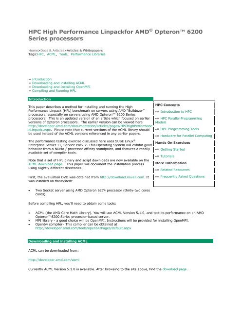
<strong>HPC</strong> <strong>High</strong> <strong>Performance</strong> <strong>Linpack</strong>for <strong>AMD</strong> ® Opteron 6200<br />
Series processors<br />
Home>Docs & Articles>Articles & Whitepapers<br />
Tags:<strong>HPC</strong>, ACML, Tools, <strong>Performance</strong> Libraries<br />
» Introduction<br />
» Downloading and installing ACML<br />
» Downloading and Installing OpenMPI<br />
» Compiling and Running HPL<br />
Introduction<br />
This paper describes a method for installing and running the <strong>High</strong><br />
<strong>Performance</strong> <strong>Linpack</strong> (HPL) benchmark on servers using <strong>AMD</strong> “Bulldozer”<br />
processors, especially on servers using <strong>AMD</strong> Opteron 6200 Series<br />
processors. This is an updated version of an article which focused on earlier<br />
versions of Opteron processors. The earlier version can be viewed here<br />
http://developer.amd.com/documentation/articles/pages/<strong>HPC</strong><strong>High</strong>Performanc<br />
e<strong>Linpack</strong>.aspx. Please note that current versions of the ACML library should<br />
be used instead of the ACML versions referenced in any earlier papers.<br />
The performance testing exercise discussed here uses SUSE Linux ®<br />
Enterprise Server 11, Service Pack 2. This Operating System will exhibit good<br />
behavior from a NUMA / processor affinity standpoint, and features a readily<br />
available set of compiler tools.<br />
Note that a set of HPL binary and script downloads are now available on the<br />
ACML download page. This paper will document the installation process<br />
using slightly different directories.<br />
First, the evaluation DVD was obtained from http://download.novell.com. It<br />
was installed on thissystem:<br />
Two Socket server using <strong>AMD</strong> Opteron 6274 processor (thirty-two cores<br />
cores)<br />
Before compiling HPL, you’ll need to obtain some tools:<br />
ACML (the <strong>AMD</strong> Core Math Library). You will use ACML Version 5.1.0, and test its performance on an <strong>AMD</strong><br />
Opteron6200 Series processor-based server.<br />
MPI library - a good choice will be OpenMPI. Instructions will be provided for installing OpenMPI.<br />
Open64 compiler– This compiler can be obtained at<br />
http://developer.amd.com/tools/open64/Pages/default.aspx<br />
Downloading and installing ACML<br />
ACML can be downloaded from:<br />
http://developer.amd.com/acml<br />
<strong>HPC</strong> Concepts<br />
» Introduction to <strong>HPC</strong><br />
» <strong>HPC</strong> Parallel Programming<br />
Models<br />
» <strong>HPC</strong> Programming Tools<br />
» Hardware for Parallel Computing<br />
Hands On Exercises<br />
» Getting Started<br />
» Tutorials<br />
More Information<br />
» Related Resources<br />
» Frequently Asked Questions<br />
Currently ACML Version 5.1.0 is available. After browsing to the site above, find the download page.
Download from the OPEN64 group:<br />
acml-5-1-0-open64-64bit.tgz<br />
As root, install ACML using the below commands:<br />
tar xzvf acml-5-1-0-open64-64bit.tgz<br />
./install-acml-5-1-0-open64-64bit.sh<br />
The install script will prompt you to accept the license agreement. The default installation locations will be in the<br />
directory/opt/acml5.1.0.<br />
NOTE: If installing to the default location, you might want to change ownership of the ACML directory and it’s<br />
subdirectories to that of a non-privileged user. This will allow that user to run the examples without needing root<br />
privilege. Otherwise, you might want to install into a user account subdirectory.<br />
NOTE: It’s a good idea to run the ACML examples to ensure that the package is installed correctly and that the<br />
compiler environment is correct. Just go to the example directory and type make. Several C and Fortran<br />
examples should build and run. That’s all you need to do for ACML.<br />
NOTE: The Gfortran version of ACML can also be used. In this case it is necessary to use the 4.6.2 version of<br />
GCC/Gfortran (or newer). <strong>Performance</strong> with Open64 is slightly better than with Gfortran.<br />
Downloading and installing OpenMPI<br />
Though an MPI may come with the Linux distribution, we want an MPI implementation that has great support for<br />
NUMA architectures and can be tweaked for a few other optimizations.<br />
A good open-source choice for MPI is OpenMPI. OpenMPI can be downloaded from:<br />
http://www.open-mpi.org (click on the “Download” link in the “Open MPI Software” menu on the left)<br />
Excellent instructions are provided on that website. There is a general FAQ and information on how to build here:<br />
http://www.open-mpi.org/faq/<br />
http://www.open-mpi.org/faq/?category=building<br />
However we’ll provide some specific instructions as well. In this case, you’ll install the MPI libraries to our home<br />
directory, assuming “hpcuser” is the home user. Otherwise, one would need to log in as root since by default<br />
OpenMPI will go into /usr/local. At a command prompt:<br />
cd ~<br />
wget http://www.open-mpi.org/software/ompi/v1.5/downloads/openmpi-<br />
1.5.5.tar.bz2<br />
tar xjfopenmpi-1.5.5.tar.bz2<br />
mkdir /home/hpcuser/openmpi-install<br />
cd /home/hpcuser/openmpi-install<br />
/home/hpcuser/openmpi-1.5.5/configure –-help<br />
/home/hpcuser/openmpi-1.5.5/configure --prefix=/home/hpcuser/openmpi-install<br />
2>&1 | tee configure.log<br />
If you do not want a parallel build, remove the “-j 20”:<br />
make –j 20 2>&1 | tee make.log
make install 2>&1 | tee make_install.log<br />
We could use more cores for building on our 32 core machines, but OpenMPI doesn’t take too long to build.<br />
Alternatively make and install can be combined with:<br />
# make all install –j 20 2>&1 | tee make_all_install.log<br />
Now, to use this MPI implementation, you would simply modify your PATHas shown below.<br />
To make sure OpenMPI will work correctly, and to make sure it will work on multiple nodes, make sure you add<br />
statements like the following to your .bashrc file:<br />
export PATH=/home/hpcuser/openmpi-install/bin:${PATH}<br />
export LD_LIBRARY_PATH=\<br />
/home/hpcuser/openmpi-install/lib:${LD_LIBRARY_PATH}<br />
After installing OpenMPI on multiple nodes, you can very quickly validate OpenMPI like this:<br />
mpirun –np2 –host host1,host2 –np2 /bin/ls<br />
If this fails, it may be because you did not modify PATHand LD_LIBRARY_PATH, in the .bashrc or<br />
/etc/profile.local on all nodes. In that case you may see errors like the following:<br />
bash: orted: command not found<br />
[node1:11985] [0,0,0] ORTE_ERROR_LOG: Timeout in file /home/hpcuser/openmpi-<br />
1.5.5/orte/mca/pls/base/pls_base_orted_cmds.c at line 275<br />
[node1:11985] ERROR: A daemon on node node2 failed to start as expected.<br />
Compiling and Running HPL - The Basics<br />
The <strong>High</strong> <strong>Performance</strong> <strong>Linpack</strong> software is obtainable from:<br />
http://www.netlib.org<br />
It’s also bundled as part of the <strong>HPC</strong> Challenge collection of software. In that case, they’ve added a few extra<br />
Makefiles illustrating various recent platforms.<br />
Basic installation instructions can be found here:http://www.netlib.org/benchmark/hpl<br />
Following is a set of commands to get going with HPL:<br />
cd /home/hpcuser<br />
wget http://www.netlib.org/benchmark/hpl/hpl-2.0.tar.gz<br />
tar xzvf hpl-2.0.tar.gz<br />
cd hpl-2.0<br />
cp setup/Make.Linux_ATHLON_FBLAS make.open64_acml<br />
vi Make.open64_acml<br />
1. Change the line with<br />
ARCH = Linux_ATHLON_FBLAS
To something like (this can be any name you want):<br />
ARCH = open64_acml<br />
2. Change the line with<br />
TOPdir = $(HOME)/hpl<br />
as required to point to the correct directory.<br />
3. Change this line:<br />
CC = /usr/bin/gcc<br />
to:<br />
CC = opencc<br />
4. Change this line:<br />
LINKER = /usr/bin/g77<br />
to:<br />
LINKER = openf90<br />
5. For OpenMPI, change these default lines:<br />
MPdir = /usr/local/mpi<br />
MPinc = -I$(MPdir)/include<br />
MPlib = $(Mpdir)/lib/libmpich.a<br />
to:<br />
MPdir = /home/hpcuser/openmpi-install<br />
MPinc = -I$(MPdir)/include<br />
MPlib =-L$(MPdir)/lib -lmpi<br />
6. For ACML 5.1.0, change these lines:<br />
LAdir = $(HOME)/netlib/ARCHIVES/Linux_ATHLON<br />
LAinc =<br />
LAlib = $(LAdir)/libf77blas.a $(Ladir)/libatlas.a<br />
to:<br />
LAdir = /opt/acml5.1.0/open64_64_fma4<br />
LAinc = -I$(LAdir)/include<br />
LAlib = $(LAdir)/lib/libacml.a<br />
Note the use of the static ACML library. Do not use the shared object library for HPL since this may result in very<br />
poor performance.
7. Last, change the default C compiler flags<br />
CCFLAGS = $(HPL_DEFS) -fomit-frame-pointer -O3 -funroll-loops -W -Wall<br />
to:<br />
= $(HPL_DEFS) –O3<br />
Now do the compile of HPL:<br />
cd /home/hpcuser/hpl-2.0<br />
make –j 8 arch=open64_acml<br />
The example above only uses 8 cores for the build. You can use more than eight cores for the build, but HPL builds<br />
very fast even with just one processor.<br />
NOTE: Remember for subsequent builds you will need to clean out the objects as in the comments below:<br />
# When changing compiler and link options,<br />
# clean out the objects before rebuilding:<br />
# make clean arch=open64_acml<br />
To run HPL with OpenMPI, you can use the following commands – and do not forget to set the PATH variable!<br />
export PATH=/home/hpcuser/openmpi-install/bin:${PATH}<br />
export LD_LIBRARY_PATH=/home/hpcuser/openmpi-install/lib<br />
cd /home/hpcuser/hpl/bin/open64_acml<br />
# Do this however you want; this way lets one know<br />
# exactly what HPL.dat generated what output.<br />
cat HPL.dat >xhpl.out<br />
mpirun –np 4 ./xhpl>>xhpl.out<br />
In the example above, np4 means to run this distributed workload on 4 processors. Running the default HPL.dat<br />
should take no more than a few seconds. The default output simply goes to stdout, which redirects to a file.<br />
Next, examine xhpl.out for the results. If it has run correctly, with the default HPL.dat, then you should see that it<br />
has run 864 tests. It’ll say that they’ve passed residual checks.<br />
To glance at the performance, simply:<br />
grep WR xhpl.out<br />
The far left-hand field “T/V” is a combination of characters that describe the possible parameter permutations.<br />
Other parameters, “N”, “NB”, “P”, and “Q” are enumerated in separate columns. Then the performance metrics;<br />
the meaning of “Time” is obvious, and it is in seconds. Finally, the metric everyone is interested in is “Gflops”<br />
on the far right. This is an aggregated throughput metric based on the estimated number of floating point<br />
calculations for a particular set of parameters, divided by time: gigaflops per second.<br />
To make it more realistic, modify HPL.dat as follows:<br />
1. Change line 6 (“Ns”, controlled by preceding line 5), from:
29 30 34 35 Ns<br />
to:<br />
10000 15000 20000 30000 Ns<br />
2. Change lines 7 and 8 (“# of NBs”, “NBs” -- block sizes and how many) from:<br />
4 # of NBs<br />
1 2 3 4 NBs<br />
to:<br />
3 # of NBs<br />
100 92 104 NBs<br />
To simplify what you arelooking at, reduce the possible permutations of how the workload is distributed and<br />
factorized.<br />
3. Change lines 10-12 [“# of process grids (P X Q)” ] from:<br />
3<br />
2 1 4 Ps<br />
2 4 1 Qs<br />
to:<br />
1<br />
4 Ps<br />
8 Qs<br />
The HPL.dat file should look like this:<br />
HP<strong>Linpack</strong> benchmark input file<br />
Innovative Computing Laboratory, University of Tennessee<br />
HPL.out output file name (if any)<br />
6 device out (6=stdout,7=stderr,file)<br />
4 # of problems sizes (N)<br />
10000 15000 20000 30000 # Ns<br />
3 # of NB<br />
100 92 104 # NBs<br />
0 PMAP process mapping (0=Row-,1=Column-major)<br />
1 # of process grids (P x Q)<br />
4 Ps<br />
8 Qs<br />
16.0 threshold<br />
1 # of panel fact<br />
2 1 PFACTs (0=left, 1=Crout, 2=Right)<br />
1 # of recursive stopping criterium<br />
4 2 NBMINs (>= 1)<br />
1 # of panels in recursion<br />
2 4 NDIVs<br />
1 # of recursive panel fact.<br />
2 1 0 RFACTs (0=left, 1=Crout, 2=Right)<br />
1 # of broadcast
1 3 BCASTs (0=1rg,1=1rM,2=2rg,3=2rM,4=Lng,5=LnM)<br />
1 # of lookahead depth<br />
0 1 2 DEPTHs (>=0)<br />
1 SWAP (0=bin-exch,1=long,2=mix)<br />
64 swapping threshold<br />
0 L1 in (0=transposed,1=no-transposed) form<br />
0 U in (0=transposed,1=no-transposed) form<br />
1 Equilibration (0=no,1=yes)<br />
8 memory alignment in double (> 0)<br />
Now rerun:<br />
cat HPL.dat > xhpl_2.out ; mpirun –np32 ./xhpl>> xhpl_2.out<br />
This will take several minutes. The output for this simple run is included at the end of this paper.<br />
In this case, np32 means to run this distributed workload on 32 processors. To make this work, the product of<br />
PxQ set in HPL.dat would need to be 32, hence the 4 and 8.<br />
A setting of np32 would be suitable for a two socket server using <strong>AMD</strong> Opteron6200 Series processors.<br />
This HPL.dat file is a suitable starting point for current <strong>AMD</strong> Opteron6200 Series processor-based servers. The<br />
parameters have been chosen to provide good performance on such systems. You can experiment with<br />
combinations of these parameters to see how they affect performance. The basic methodology is to systematically<br />
try different parameters to see which ones provide the highest Gflops result. In general, do so with small problems<br />
(~10000) which run quickly. You can run a lot of experiments in short time this way. Refer to the tuning guide on<br />
the HPL web page for more information. Another useful reference is this description of the HPL benchmark. It<br />
helps to know how the code works when trying to tune it.<br />
Example Results<br />
Here are the results of running HPL on a Dinar platform with the HPL.dat parameters described above. These<br />
performance results are for smaller problems and are not representative of what can be achieved with larger<br />
problems.<br />
Note that slightly better performance can be obtained for benchmarking and stress test purposes by turning off<br />
APM mode in the BIOS settings. This will force the processor to remain in the primary voltage/frequency state.<br />
Among the benefits of this is more consistency in the results. A similar BIOS change is to enable <strong>HPC</strong> mode if it is<br />
available. <strong>HPC</strong> mode sets most of the power management P-States to the same value, while still allowing higher<br />
frequency Boost P-States. If your BIOS does not have a <strong>HPC</strong> mode option, a simple hpcmode clock configuration<br />
utility can be downloaded from http://developer.amd.com/libraries/acml/downloads/pages/default.aspx. For a full<br />
description of the Advanced Power Management features of the <strong>AMD</strong> Opteron 6200 Series processors, refer to<br />
the BIOS and Kernel <strong>Developer</strong>s Guide (BKDG) for <strong>AMD</strong> Family 15h Models 00h-0fh processors.<br />
Notice how the choice of NB makes a big difference in performance. The best number, 100, is specific to ACML on<br />
these processors, other NBs will be used with other combinations of libraries and CPUs. Ideally, N should be a<br />
even multiple of NB.<br />
mpirun -n 32 xhpl<br />
=============================================================================<br />
HP<strong>Linpack</strong>2.0 -- <strong>High</strong>-<strong>Performance</strong> <strong>Linpack</strong> benchmark -- September 10, 2008<br />
Written by A. Petitet and R. Clint Whaley, Innovative Computing Laboratory,<br />
UTK<br />
Modified by Piotr Luszczek, Innovative Computing Laboratory, UTK<br />
Modified by JulienLangou, University of Colorado Denver<br />
=============================================================================
An explanation of the input/output parameters follows:<br />
T/V : Wall time / encoded variant.<br />
N : The order of the coefficient matrix A.<br />
NB : The partitioning blocking factor.<br />
P : The number of process rows.<br />
Q : The number of process columns.<br />
Time : Time in seconds to solve the linear system.<br />
Gflops : Rate of execution for solving the linear system.<br />
The following parameter values will be used:<br />
N : 10000 15000 20000 30000<br />
NB : 92 104 100<br />
PMAP : Row-major process mapping<br />
P : 4<br />
Q : 8<br />
PFACT : Right<br />
NBMIN : 4<br />
NDIV : 2<br />
RFACT : Right<br />
BCAST : 1ringM<br />
DEPTH : 0<br />
SWAP : Spread-roll (long)<br />
L1 : transposed form<br />
U : transposed form<br />
EQUIL : yes<br />
ALIGN : 8 double precision words<br />
-----------------------------------------------------------------------------<br />
- The matrix A is randomly generated for each test.<br />
- The following scaled residual check will be computed:<br />
||Ax-b||_oo / ( eps * ( || x ||_oo * || A ||_oo + || b ||_oo ) * N )<br />
- The relative machine precision (eps) is taken to be<br />
1.110223e-16<br />
- Computational tests pass if scaled residuals are less than 16.0<br />
=============================================================================<br />
T/V N NB P Q Time Gflops<br />
-----------------------------------------------------------------------------<br />
WR01R2R4 10000 92 4 8 4.28 1.558e+02<br />
-----------------------------------------------------------------------------<br />
||Ax-b||_oo/(eps*(||A||_oo*||x||_oo+||b||_oo)*N)= 0.0035143 ... PASSED<br />
=============================================================================<br />
T/V N NB P Q Time Gflops<br />
-----------------------------------------------------------------------------<br />
WR01R2R4 10000 104 4 8 4.34 1.536e+02<br />
-----------------------------------------------------------------------------<br />
||Ax-b||_oo/(eps*(||A||_oo*||x||_oo+||b||_oo)*N)= 0.0035900 ... PASSED<br />
=============================================================================<br />
T/V N NB P Q Time Gflops<br />
-----------------------------------------------------------------------------<br />
WR01R2R4 10000 100 4 8 4.28 1.557e+02<br />
-----------------------------------------------------------------------------<br />
||Ax-b||_oo/(eps*(||A||_oo*||x||_oo+||b||_oo)*N)= 0.0031279 ... PASSED<br />
=============================================================================<br />
T/V N NB P Q Time Gflops<br />
-----------------------------------------------------------------------------<br />
WR01R2R4 15000 92 4 8 12.63 1.781e+02<br />
-----------------------------------------------------------------------------
||Ax-b||_oo/(eps*(||A||_oo*||x||_oo+||b||_oo)*N)= 0.0033686 ... PASSED<br />
=============================================================================<br />
T/V N NB P Q Time Gflops<br />
-----------------------------------------------------------------------------<br />
WR01R2R4 15000 104 4 8 12.92 1.742e+02<br />
-----------------------------------------------------------------------------<br />
||Ax-b||_oo/(eps*(||A||_oo*||x||_oo+||b||_oo)*N)= 0.0029765 ... PASSED<br />
=============================================================================<br />
T/V N NB P Q Time Gflops<br />
-----------------------------------------------------------------------------<br />
WR01R2R4 15000 100 4 8 12.59 1.787e+02<br />
-----------------------------------------------------------------------------<br />
||Ax-b||_oo/(eps*(||A||_oo*||x||_oo+||b||_oo)*N)= 0.0030555 ... PASSED<br />
=============================================================================<br />
T/V N NB P Q Time Gflops<br />
-----------------------------------------------------------------------------<br />
WR01R2R4 20000 92 4 8 28.21 1.891e+02<br />
-----------------------------------------------------------------------------<br />
||Ax-b||_oo/(eps*(||A||_oo*||x||_oo+||b||_oo)*N)= 0.0025704 ... PASSED<br />
=============================================================================<br />
T/V N NB P Q Time Gflops<br />
-----------------------------------------------------------------------------<br />
WR01R2R4 20000 104 4 8 28.75 1.855e+02<br />
-----------------------------------------------------------------------------<br />
||Ax-b||_oo/(eps*(||A||_oo*||x||_oo+||b||_oo)*N)= 0.0027287 ... PASSED<br />
=============================================================================<br />
T/V N NB P Q Time Gflops<br />
-----------------------------------------------------------------------------<br />
WR01R2R4 20000 100 4 8 27.93 1.909e+02<br />
-----------------------------------------------------------------------------<br />
||Ax-b||_oo/(eps*(||A||_oo*||x||_oo+||b||_oo)*N)= 0.0023810 ... PASSED<br />
=============================================================================<br />
T/V N NB P Q Time Gflops<br />
-----------------------------------------------------------------------------<br />
WR01R2R4 30000 92 4 8 88.42 2.036e+02<br />
-----------------------------------------------------------------------------<br />
||Ax-b||_oo/(eps*(||A||_oo*||x||_oo+||b||_oo)*N)= 0.0029272 ... PASSED<br />
=============================================================================<br />
T/V N NB P Q Time Gflops<br />
-----------------------------------------------------------------------------<br />
WR01R2R4 30000 104 4 8 90.17 1.996e+02<br />
-----------------------------------------------------------------------------<br />
||Ax-b||_oo/(eps*(||A||_oo*||x||_oo+||b||_oo)*N)= 0.0025377 ... PASSED<br />
=============================================================================<br />
T/V N NB P Q Time Gflops<br />
-----------------------------------------------------------------------------<br />
WR01R2R4 30000 100 4 8 87.86 2.049e+02<br />
-----------------------------------------------------------------------------<br />
||Ax-b||_oo/(eps*(||A||_oo*||x||_oo+||b||_oo)*N)= 0.0025044 ... PASSED<br />
=============================================================================<br />
Finished 12 tests with the following results:<br />
12 tests completed and passed residual checks,<br />
0 tests completed and failed residual checks,<br />
0 tests skipped because of illegal input values.<br />
-----------------------------------------------------------------------------<br />
End of Tests.
<strong>AMD</strong>, the <strong>AMD</strong> logo, the Arrow logo and <strong>AMD</strong> Opteron and combinations thereof are registered trademarks of<br />
Advanced Micro Devices, Inc. in the U.S. and other jurisdictions.<br />
Linux® is the registered trademark of Linus Torvalds in the U.S. and other countries.<br />
Other names are information purposes only and may be trademarks of their respective owners.


