Learning manifolds of dynamical models for activity recognition

of the manifold. Consider then an automorphism (invertible
differentiable map) between M and itself: F : M → M,
m ↦→ F (m), m ∈ M. Let us denote by TmM the tangent
space to M in m. Each tangent vector v ∈ TmM maps any
function f on M to the derivative of f along the direction
v: v(f) = ∂f/∂v.
Any automorphism F is associated with a push-forward
map of tangent vectors: F∗ : TmM → T F (m)M, v ∈
TmM ↦→ F∗v ∈ T F (m)M defined as F∗v(f) = v(f ◦ F )
for all smooth functions f on M, which maps f to its partial
derivative ∂f/∂v in F (m).
Consider now a Riemannian metric 1 g : T M × T M → R
on M. The automorphism F induces a pullback metric
on M: g∗m(u, v) . = g F (m)(F∗u, F∗v) such that the scalar
product of two tangent vectors u, v in m ∈ M according to
the pullback metric g∗ is the scalar product with respect to
the original metric g of the push-forward vectors F∗u, F∗v
in F (m). The pullback geodesic (shortest path) between
two points is the lifting of the geodesic connecting their images
with respect to the original metric. A pullback distance
between two points on M (in our case, two dynamical models)
can be computed along such pullback geodesic.
By defining a class of such automorphisms {Fλ, λ ∈ Λ}
depending on some parameter λ, we get a corresponding
family of pullback metrics {g∗λ, λ ∈ Λ} on M. We can
then define an optimization problem over such family in order
to select an “optimal” metric. The nature of the resulting
manifold will obviously depend on the objective function
we choose to optimize.
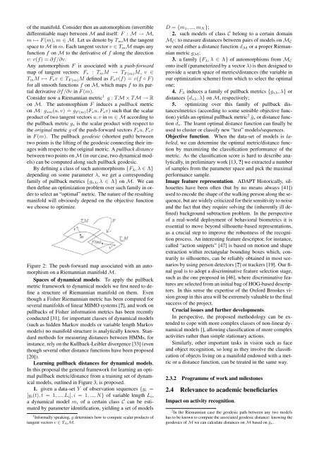
Figure 2: The push-forward map associated with an automorphism
on a Riemannian manifold M.
Spaces of dynamical models. To apply the pullback
metric framework to dynamical models we first need to define
a structure of Riemannian manifold on them. Even
though a Fisher Riemannian metric has been computed for
several manifolds of linear MIMO systems [?], and work on
pullbacks of Fisher information metrics has been recently
conducted [31], for important classes of dynamical models
(such as hidden Markov models or variable length Markov
models) no manifold structure is analytically known. Standard
methods for measuring distances between HMMs, for
instance, rely on the Kullback-Leibler divergence [33] (even
though several other distance functions have been proposed
[20]).
Learning pullback distances for dynamical models.
In this proposal the general framework for learning an optimal
pullback metric/distance from a training set of dynamical
models, outlined in Figure 3, is proposed.
1. given a data-set Y of observation sequences {yi =
[yi(t), t = 1, ..., Li], i = 1, ..., N} of variable length Li,
a dynamical model mi of a certain class C can be estimated
by parameter identification, yielding a set of models
1 Informally speaking, g determines how to compute scalar products of
tangent vectors v ∈ TmM.
D = {m1, ..., mN};
2. such models of class C belong to a certain domain
MC: to measure distances between pairs of models on MC
we need either a distance function dM or a proper Riemannian
metric gM;
3. a family {Fλ, λ ∈ Λ} of automorphisms from MC
onto itself (parameterized by a vector λ) is then designed to
provide a search space of metrics/distances (the variable in
our optimization scheme) from which to select the optimal
one;
4. Fλ induces a family of pullback metrics {g∗λ, λ} or
distances {d∗λ, λ} on M, respectively;
5. optimizing over this family of pullback distances/metrics
(according to some sensible objective function)
yields an optimal pullback metric 2 ˆg∗ or distance function
ˆ d∗. The learnt optimal distance function can finally be
used to cluster or classify new “test” models/sequences.
Objective function. When the data-set of models is labeled,
we can determine the optimal metric/distance function
by maximizing the classification performance of the
metric. As the classification score is hard to describe analytically,
in preliminary work [13, ?] we extracted a number
of samples from the parameter space and pick the maximal
performance sample.
Image feature representation. ADAPT Historically, silhouettes
have been often (but by no means always [41])
used to encode the shape of the walking person along the sequence,
but are widely criticized for their sensitivity to noise
and the fact that they require solving the (inherently ill defined)
background subtraction problem. In the perspective
of a real-world deployment of behavioral biometrics it is
essential to move beyond silhouette-based representations,
as a crucial step to improve the robustness of the recognition
process. An interesting feature descriptor, for instance,
called “action snippets” [47] is based on motion and shape
extraction within rectangular bounding boxes which, contrarily
to silhouettes, can be reliably obtained in most scenarios
by using person detectors [?] or trackers [19]. Our final
goal is to adopt a discriminative feature selection stage,
such as the one proposed in [46], where discriminative features
are selected from an initial bag of HOG-based descriptors.
In this sense the expertise of the Oxford Brookes vision
group in this area will be extremely valuable to the final
success of the project.
Crucial issues and further developments.
In perspective, the proposed methodology can be extended
to cope with more complex classes of non-linear dynamical
models [], allowing classification of more complex
activities rather than simple stationary actions.
Similarly, other important tasks in vision such as face
and object recognition, so long as they involve the classification
of objects living on a manifold endowed with a metric
or a distance function, can be treated in the same way.
2.3.2 Programme of work and milestones
2.4 Relevance to academic beneficiaries
Impact on activity recognition.
2 In the Riemannian case the geodesic path between any two models
has to be known to compute the associated geodesic distance: knowing the
geodesics of M we can calculate distances on M based on ˆg∗.