Final Copy - Oxford Brookes University

A Novel Approach for Video Quantization
Using the Spatiotemporal Frequency
Characteristics of the Human Visual System
Branko Petljanski and Oge Marques
Department of Computer Science and Engineering
Florida Atlantic University
Boca Raton, FL, 33431, USA
branko@voyager.ee.fau.edu, omarques@fau.edu
Abstract
The temporal limitations of the human visual system (HVS) are usually not
fully explored in the quantization stage of today’s video encoders. In this paper
we present a novel method to improve the compression efficiency of popular
video compression algorithms in which the temporal frequency response
characteristics of the HVS are taken into account while building macroblockspecific
quantization matrices for non-intra-coded (i.e., ‘P’ or ‘B’) frames.
These quantization matrices help removing redundant information from the
video sequence and, consequently, increase compression efficiency. Results
from our experiments show that the proposed approach can achieve improved
bit savings over a standard encoder without sacrificing the perceived visual
quality of the compressed sequence.
1 Introduction
Contemporary video compression algorithms use an encoding strategy in which frames
are organized in GOPs (Groups of Pictures), usually of the form ‘IPPBPPI’... or any
of its common variants. Frames coded as stand-alone frames are called ‘I’ or intra(coded)
frames. ‘P’ stands for predicted frames, which are coded relatively to the nearest
previous ‘I’ or ‘P’ frame. Finally, ‘B’ or bidirectional frames use the closest ‘I’ or ‘P’
frame as a reference. For intra-coded frames, the frame is divided into blocks of 8 × 8
pixels. Blocks are then transformed using the Discrete Cosine Transform (DCT) into the
frequency domain for better energy compaction. Transformed blocks are quantized using
a weighted quantization matrix (QM) that appropriately maps the spatial limitations of
the Human Visual System (HVS).
For ‘P’ and ‘B’ frames, the encoding process includes a motion estimation (ME) step,
which consists of predicting the most likely location for a macroblock (MB) from the
reference frame in the target frame. While encoding the differences (errors) between
intensity values at current location and predicted location, most popular algorithms use a
QM that weights all residual DCT coefficients within a block equally. This QM does not
take into account the fact that depending on the spatial displacement between the current

and predicted locations of a block – and, therefore, of its perceived speed – the human
eye will give more or less importance to the block’s contents.
This paper presents a novel method to improve the compression efficiency of DCTbased
video compression algorithms without perceivable quality loss. Under the proposed
approach, temporal frequency response characteristics of the HVS are taken into account
in order to build a quantization matrix for each block in non-intra (i.e., ‘P’ or ‘B’) frames.
These quantization matrices remove redundant information from the video sequence and
consequently increase compression efficiency. The exploitation of temporal limitations
of HVS, in addition to the exploitation of spatial limitations included in the baseline algorithm
– can result in improved bit savings over the baseline case without sacrificing the
perceived visual quality of the compressed sequence. The proposed method is also capable
of reconstructing the quantization matrix for each block on the decoder side without
increasing bit overhead.
This paper is organized as follows: Section 2 presents the basic concepts and assumptions
behind our work. Section 3 describes the proposed method, while Section 4 shows
results of our experiments. Finally, Section 5 concludes the paper.
2 Background
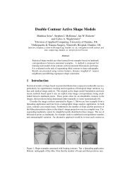
Modern video compression algorithms use temporal redundancy to increase the compression
efficiency for non-intra-coded frames. Figure 1 depicts a general block diagram of an
MPEG encoder and decoder, where the grayed blocks are related to the work described
in this paper. A motion estimator (ME) uses the reference frame stored in a buffer to
compare it with the current frame from the video stream to find similar blocks between
them. The position of the block in the currently coded frame relative to the block in
the reference frame is described by a motion vector (MV). Only one frame per GOP is
intra-coded, while others are only described with MVs and intensity differences between
blocks. These differences are transformed to the frequency domain using a mathematical
transform such as the two-dimensional DCT.
Figure 1: Block diagrams of general MPEG encoder and decoder.
The frequency domain characterizes better energy compaction. At this point, the decoder
can recover the encoded frames without any loss in information – encoding is loss-

less, but compression efficiency is low. Special attention is given to the quantizer stage
(Q in the diagram). For intra-coded frames, a weighted quantization matrix (QM) maps
the spatial limitations of the HVS to perceive high frequency of an image into a low-pass
filter. Most of the high frequency contents are significantly attenuated, under the assumption
that the observer will not be able to notice them anyway. In non-intra-coded frames,
a flat quantization matrix – that attenuates all frequencies by the same amount – is typically
used. After the quantization process, the encoded frame cannot be reconstructed as
the original any longer, because some information has been lost. Compression is lossy,
but compression efficiency is higher. The goal of a good compression algorithm is to
find the right balance between perceived artifacts in decoded frame and compression efficiency.
Our work proposes a novel approach in constructing quantization matrices using
the temporal frequency limitations of HVS for non-intra-coded frames that yields additional
compression efficiency without adding perceivable artifacts in the decoded image.
Local bit allocation in a reference MPEG encoder is based on two measurements:
deviancy from estimated buffer fullness and normalized spatial activity. Combination of
these two measurements results in appropriate modification of the gain of flat quantization
matrices [7].
Various adaptive quantization methods have been proposed. In [8], a strategy for
adaptive quantization in an MPEG encoder based on HVS properties is discussed. Under
the authors’ proposed approach, MBs are classified in regard to their visual importance
and tolerance for compression. A distinction is made between MBs that contain edges
as opposed to MBs containing textures. The algorithm uses the fact that the HVS is
more sensitive to compression errors coming from the edges of an object. The paper also
briefly discusses classification of regions with rapid or smooth motion, and asserts that
rapid motion cannot be tracked so it can tolerate significant quantization due to temporal
masking.
In a related work, Malo et. al. [5] proposed the use of temporal filtering to improve
quantization in intra-coded frames. One of the practical difficulties with their approach is
that the implementation of the proper temporal filters requires storage of multiple frames.
Our approach uses only the reference and current frames to implement temporal filtering.
Since they are already available to the encoder, no additional storage resources are
required.
In [6], the authors stated that – due to camera integration – real video systems tend
to blur the picture in areas of high motion, which would make the gain from coarser
quantization probably be modest. Camera integration is controlled by a shutter mechanical
mechanism or, in new cameras, by an electronic shutter. Modern CCD and CMOS
imagers have greatly improved sensitivity and shorter integration time, which leads to
smaller blur of high motion.
In [1], Girod observes that smooth pursuit of moving objects reduces the effective
temporal frequency. In the ideal case, the temporal frequency at the retina is zero. Perfect
eye tracking is possible only under special conditions (i.e. smoothly moving object in a
simple scene whose movement observer can predict) due to delay in human reaction and
saccades [2].
In this paper, we assume that such conditions are rarely present in real scenes, which
usually consist of one or multiple moving objects with erratic movement. Under such
conditions, the observer has limited capabilities to smoothly track a moving object and
consequently reduce temporal frequencies.

3 The proposed method
In this Section we explain the rationale behind the proposed approach and present relevant
related calculations.
3.1 Spatiotemporal frequency characteristic of the HVS
The most influential work in the area of spatiotemporal frequency characteristic of the
HVS was published by D.H. Kelly [4]. In his work, Kelly claims that, under certain
assumptions, the HVS has a distinctive response in both spatial and temporal domains.
The spatial frequency response describes visual sensitivity to a stationary spatial pattern
with different spatial frequency, whereas the visual sensitivity to a temporally varying
pattern at different frequencies is described as the temporal frequency response of HVS.
In addition to the frequency dependency, the temporal frequency response of HVS is also a
function of the mean brightness level in a scene. Kelly’s results are reproduced in Figure 2,
where it can be seen that for a constant brightness level, the temporal frequency response
of the HVS behaves like a low-pass filter. This low-pass characteristic of the HVS means
that, beyond a certain point, it is not able to discriminate any spatial variations in a given
block.
Figure 2: The temporal frequency response of the HVS (adapted from [4]) where it can
be seen that high temporal frequencies are attenuated.
3.2 Preliminary calculations
Suppose that an object in a frame is moving with horizontal and vertical velocity, vx and vy
respectively. If the spatial pattern of the object is characterized by horizontal and vertical
frequencies ( fx, fy), then the apparent temporal frequency can be calculated as:
ftemporal = − fxvx − fyvy
(1)

The apparent temporal frequency of the observed object is a function of velocity and
frequency content of the object. The upper bound on a temporal frequency of a moving
object is achieved when a maximum velocity vector and a maximum spatial frequency
content occur simultaneously. In MPEG-like coding schemes, the velocity of an object
can be determined only if the best match is found within the search region in the subsequent
frames. Suppose that the search region is a rectangular area of size 36 × 36 pixels.
Objects that travel the maximum spatial distance between two consecutive frames will
have maximum velocity. The maximum spatial distance that an object can travel is obtained
when the best match is at the edge of the search region.
Assuming progressive scan at 30 frames per second and CIF (Common Intermediate
Format) video frame size (352 × 288 pixels), we can calculate the maximum speed of an
object by dividing the maximum distance that the object travels by the minimum possible
time interval (the reciprocal of the frame rate, in this case):
vmax = dmax/33.3ms = ( 18pixels
352pixels )(
1
) = 1.53screen width/s (2)
33.3ms
If the observed object is a block of size 16 × 16 pixels, then the maximum spatial
frequency for such a block is 8 cycles/length. Using these assumptions, the maximum
spatial frequency expressed in cycles per screen width is:
fspatialmax =
8cycles
= 176cycles/screen width (3)
16pixels/352pixels
If the maximum velocity vector and the maximum spatial frequency occur simultaneously,
the maximum temporal frequency can be determined using ( 1):
ftemporalmax = vmax × fspatialmax = 1.53 × 176 = 270Hz (4)
The maximum temporal frequency of 270 Hz serves as an upper bound and it is clearly
higher than the cutoff frequency of all curves shown in Figure 2. This is due to the assumption
that an object with the maximum spatial frequency is moving with the maximum
velocity between two consecutive frames. The calculated value for maximum temporal
frequency clearly points out that the HVS is not able to discriminate higher frequencies
of the objects with high velocity, which implies that preserving all the spatial details in
the form of DCT coefficients of fast moving objects is unnecessary.
3.3 Choosing the appropriate curve
A closer inspection at Figure 2 shows that the frequency response is a function of the
mean brightness level, expressed in trolands. It is important to determine which subset
of curves should be used for a given display system. A troland (Td) is a unit of retinal
illumination equal to object luminance (in cd/m 2 ) times the pupillary aperture area (in
mm 2 ) [10]. Retinal illumination depends on the source’s capability to radiate light and the
aperture of the observer’s pupil.
Pupil diameter varies from 2 mm in very bright conditions (exceeding 54000 lux) to
8 mm under dark conditions. It has been reported that mean pupils diameter for normal
light conditions (light intensity between 2700 and 5400 lux) is 3.6 mm [9]. Multiplying
the mean pupil diameter for normal light conditions and radiating power of displaying
devices – cathode ray tube (CRT), liquid crystal display (LCD), plasma and digital light

CRT LCD Plasma DLP
1790 Td 4354 Td Max Backlight 2156 Td 5% APL 3652 Td
1627 Td Min Backlight 1353 Td 25% APL
824 Td 50% APL
539 Td 100% APL
Table 1: Illumination of human retina from various displaying systems under normal light
conditions (light intensity 2700-5400 lux).
processor (DLP) – gives illumination of human retina summarized in Table 1. It can be
seen from Table 1 that under normal viewing conditions and brightness control set to half
of the maximum value, illumination of human retina is in the range between 250 to 2100
trolands. The subset of curves that is suitable for using under normal lighting conditions
and modern displaying devices are the ones between 77 and 9300 trolands in Figure 2,
which are very close to each other.
3.4 Building a temporal quantization matrix for a non-intra
macroblock
When the prediction error information is calculated as a difference between the intra
and predicted non-intra macroblocks, an appropriate number of bits is allocated to encode
the residual coefficients. Since the transformed residual coefficients are not directly
viewed [10], it is not appropriate to use a spatial perceptually weighted QM like
the one used for intra macroblocks. Therefore, video compression standards assume a
scalar quantizer for non-intra macroblocks [11, 3], which results in a flat QM – that is,
constant number of bits for all entries. This flat QM does not include temporal nonlinear
characteristics of the HVS and attenuates all frequencies of residual coefficients in a
nondiscriminatory way.
An example might help understanding the meaning and possible use of Figure 2. Let
us observe three macroblocks, MB1, MB2 and MB3 with the same cosine grating at a
frequency of 4 cycles/width and an orientation of 45 degrees. Let us also assume that
these three macroblocks travel the same distance between two consecutive frames in the
direction shown in Figure 3.
Macroblock MB1 moved four pixels in the horizontal and four pixels in the vertical
direction during one frame period. The velocity vector of macroblock MB1 is normal to
the cosine grating and it can be projected on horizontal and vertical axis. Under these
conditions, the horizontal and vertical components are v1 x = 0.34m/s and v1 y = 0.34m/s.
Macroblock MB2 moved four pixels in the horizontal direction and four pixels in the
vertical direction but in the opposite direction than MB1, which resulted in velocity components
v2 x = 0.34m/s and v2 y = −0.34m/s. Finally, MB3 moved four pixels only in the
horizontal direction, which gives v3 x = 0.34m/s and v3 y = 0m/s.
Based on equation ( 1), the temporal frequencies for these macroblocks are, respectively,
f 1
temporal = 60 Hz, f 2
temporal = 0 Hz, and f 3
temporal = 30 Hz. The apparent modulation
of the moving grating pattern is attenuated in the case of MB1 to about 10% of the original
value, whereas in the case of MB3 it is attenuated to about 70% of the original value.
The temporal frequency of MB2 is 0Hz, which results in no attenuation.

Figure 3: Three macroblocks with the same cosine grating and velocity, but various directions.
Figure 4: Three macroblocks with the same pattern and velocity but various directions.
Frequency content of each macroblock is evenly distributed in the spectrum.
Let us expand the preceding discussion to macroblocks that have more than one frequency.
Suppose that all frequencies are equally present in a macroblock. Examples
of such macroblocks are shown in Figure 4. Attenuation of a particular frequency depends
on a macroblock’s velocity and direction. Let us assume that macroblock MB1
moved four pixels in horizontal and four pixels in vertical direction during one frame period
time. Figure 5 (left) shows the perceived attenuation of frequencies in MB1. Let
us assume that MB2 moved in the vertical direction during one frame period time. The
horizontal velocity of MB2 is zero, which yields a zero horizontal temporal frequency.
The observer will perceive only attenuation of vertical frequencies, while horizontal frequencies
will be perceived unchanged (Figure 5 (middle)). If a macroblock moves in the
horizontal direction, like MB3, then the vertical velocity is zero and the corresponding
vertical temporal frequency is zero too. That results in a perceived attenuation of horizontal
frequencies while vertical frequencies will be perceived unchanged (Figure 5 (right)).
The main premise of this work is to transfer or store only video information that will be
perceived by the end user. Using the motion vector of a macroblock, we can generate a
non-intra quantization matrix for each macroblock that will attenuate frequencies that are
not perceivable. The QM will change shape as a function of the velocity and direction
of a macroblock (Figure 6). For example, the non-intra QM for MB1 from Figure 4 will
have a shape that is the upside-down equivalent of Figure 5 (left). The same quantizer
matrices can be reconstructed at the receiver’s side, since motion vector information is
also available on decoder. Therefore, there is no need to send or store these matrices.

Figure 5: Perceived attenuation of frequencies for macroblocks shown in Figure 4. The
X- and Y-axis represent DCT coefficients that can be translated to temporal frequency.
Left: MB1; middle: MB2; right: MB3.
Figure 6: Quantization matrices for our approach.
4 Experiments and results
Experiments were performed on a standard PC with MPEG1 code written in C by one
of the authors. The video sequence used for experiment was ‘foreman’ in QCIF frame
format executed at 30 frames per second. This sequence was chosen because it combines
segments with very little motion with panning sequences and sudden (hand) movements.
The baseline reference codec – henceforth referred to as FlatMPEG – utilizes a constant
quantizer matrix, as explained in [3]. Our approach – which will be called HVSMPEG –
calculates a quantizer matrix based on the estimated motion vector for each macroblock.
The maximum gain in a quantizer matrix was set to be equal to the gain in constant
quantizer matrix of FlatMPEG.
4.1 Representative results and related comments
Quantitative results from our preliminary experiments are summarized in Table 2. It can
be seen that the biggest compression gain is achieved in the clip with reference frame
200. In the consecutive frame, the camera executes a panning of the scene, which results
in all macroblocks having certain velocity. The least compression gain is in the clip
with reference frame 0. In consecutive frames there is little motion, so only a limited
number of macroblocks experience velocity. Not surprisingly, if there is no motion in
the consecutive frames, there is no temporal frequency redundancy and consecutively no
compression gain based on it.
From a perceptual viewpoint, the most significant loss is present after frame 154 since

Figure 7: Decompressed frame 155 with detail. Left: decompressed FlatMPEG; right:
decompressed HVSMPEG .
the foreman moves his hand. Figure 7 shows both decompressed frames 155 with enlarged
details. An observer does not, however, perceive any degradation in this frame if it is
played at nominal frame rate with other following frames, because of the aforementioned
HVS temporal limitations.
5 Conclusions
We have proposed and demonstrated a novel approach to video quantization that exploits
the temporal limitations of the human visual system. This method can be applied to
the coding of non-intra-coded frames in a standard video encoder, with the following
advantages over existing solutions: (i) it does not require any additional frame storage;
(ii) the quantization matrices do not need to be transmitted; they can be generated at
the decoder’s side, instead; (iii) it provides additional bit savings; and (iv) the additional
quality loss it introduces cannot be perceived by the end user when the video clip is played
at nominal frame rate. The proposed solution has been subject to preliminary tests which
confirm the claimed bit savings as well as the associated – but not perceived – spatial
quality loss.

Reference Current FlatMPEG HVSMPEG Compression
Frame Frame Bits/Frame Bits/Frame Gain (dB)
0 1 65755 61150 0.31
0 2 66989 61658 0.36
0 3 79029 75609 0.19
154 155 73459 60417 0.84
154 156 85478 71751 0.76
154 157 87332 77245 0.53
200 201 69330 33110 3.21
200 202 85585 56881 1.77
200 203 92100 72484 1.04
Table 2: Quantitative comparison for three clip segments with little motion (upper third),
localized motion (middle third), and multiple motion (lower third) in the scene.
References
[1] B. Girod. Motion Analysis and Image Sequence Processing. Kluwer Academic
Publisher, 1993.
[2] P.E. Hallett. Handbook of Perception and Human Performance. John Wiley and
Sons, 1986.
[3] K. Jack. Video Demystified. LLH Technology Publishing, 2001.
[4] D.H. Kelly. Motion and vision ii. stabilized spatio-temporal threshold surface. J.
Opt. Soc. Am., 69:1340–1349, 1979.
[5] J. Malo, J. Gutierrez, I. Epifanio, F. Ferri, and J. Artigas. Perceptual feedback in
multigrid motion estimation using an improved DCT quantization. IEEE Transactions
on Image Processing, 10(10), October 2001.
[6] J.L. Mitchell, W.B. Pennebaker, C.E. Fogg, and D.J. LeGall. MPEG video compression
standard. International Thompson Publishing, 1996.
[7] MPEG-2. Draft - Test model 5. ISO/IEC JTC1/SC29/WG11, N0400, April 1993.
[8] W. Osberger, S. Hammond, and N. Bergmann. An MPEG encoder incorporating
perceptually based quantization. IEEE TENCON, Speech and Imaging Technologies
for Computing and Telecommunications, pages 731–733, 1997.
[9] C. A. Padgam and J.E. Saunders. The Perception of Light and Colour. G.Bell &
Sons, 1975.
[10] C. Poynton. Digital Video and HDTV Algorithms and Interface. Morgan Kaufmann
Publishers, 2003.
[11] I. Richardson. H.264 and MPEG-4 Video Compression. Wiley, 2004.