Reconstructing relief surfaces - Oxford Brookes University

400 G. Vogiatzis et al. / Image and Vision Computing 26 (2008) 397–404
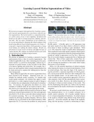
configurations of base surface and sample points (Fig. 1
right).
3. Optimisation
The MRF model laid out in the previous section provides
a probability for any possible height labelling and
corresponding relief surface. MRF inference involves
recovering the most probable site labelling which is an
NP-hard optimization problem in its generality [15]. Fortunately
a number of efficient approximate algorithms have
been proposed such as graph cuts [1] and belief propagation
[24]. These methods have been shown to give very
good results in a depth-map setting (see [21,25] for a comparison).
In this work we choose to apply a belief propagation
scheme which we outline in the following section.
3.1. Loopy belief propagation
Belief propagation works by the circulation of messages
across neighbouring sites. Each site sends to each of its
neighbours a message with its belief about the probabilities
of a neighbour being assigned a particular height. The clique
potentials
UkðhkÞ ¼exp ð CkðhkÞÞ
ð5Þ
and
Wklðhk; hlÞ ¼exp ð Cklðhk; hlÞÞ
ð6Þ
are precomputed and stored as L · 1 and L · N matrices,
respectively. Now suppose that mij(hj) denotes the message
sent from sample point i to sample point j (this is a vector
indexed by possible heights at j). We chose to implement
the max-product rule according to which, after all messages
have been exchanged, the new message sent from k to l is
emkl ¼ max UkðhkÞWklðhk; hlÞ
hk
Y
mikðhkÞ: ð7Þ
i2NðkÞ flg
The update of messages can either be done synchronously
after all messages have been transmitted, or asynchronously
with each sample point sending messages using all
the latest messages it has received. We experimented with
both methods and found the latter to give speedier convergence,
which was also reported in [25].
3.2. Coarse to fine strategy
One of the limitations of loopy belief propagation is that
it has significant memory requirements, especially as the
size of the set of possible heights is increased. In the near
future bigger and cheaper computer memory will make this
problem irrelevant, but for the system described in this
paper we designed a simple coarse to fine strategy that
allows for effective height resolutions of thousands of possible
heights. This strategy effectively, instead of considering
one BP problem with L different labels, considers
logL/logl problems with l labels where l L. It therefore
also offers a runtime speedup since it reduces the time
required from O(ML 2 )toO(logL Ml 2 /logl).
Initially the label set for all sites corresponds to a coarse
quantization of the allowable height range. After convergence
of the Belief Propagation algorithm each site is
assigned a label. In the next iteration a finer quantization
of the heights is used within a range centered at the optimal
label of the previous iteration. The label set is now allowed
to be different for each site. At each phase the number of
possible heights per node is constant but the height resolution
increases.
To make this idea more precise, at this point we replace
height labels with height range labels. A sample point can
now be labelled by a height range in which its true height
should lie. The cost for assigning height interval [Hi,Hi+1] to the kth site is now defined as:
^Ck ð½Hi; H iþ1ŠÞ
¼ min CkðhÞ: ð8Þ
h2½H i;H iþ1Š
In practice this minimum is computed by densely sampling
Ck(h) over the maximum range [Hmin,Hmax] so that the
images are all sampled at a sub-pixel rate. This computation
only has to be performed at the beginning of the algorithm.
Similarly the smoothness cost for assigning height
ranges [Hi,Hi+1], [Hj,Hj+1] to two neighbouring sites k
and l is:
^Cklð½H
H i þ H iþ1
i; H iþ1Š; ½H j; H jþ1ŠÞ ¼ Ckl
;
2
H j þ H jþ1
:
2
ð9Þ
When belief propagation converges, each point is assigned
an interval in which its height is most likely to lie. This
interval will then be subdivided into smaller subintervals
which become the site’s possible labels. The process repeats
until we reach the desired height resolution.
4. Results
In this section, a quantitative analysis using an artificial
scene with ground truth is provided. Results on a challenging
low-relief scene of a Roman sarcophagus, a building
facade and a stone carving are also illustrated. The weight
parameters w 1 and w 2 of Eqs. 3 and 4 are empirically set
relatively easily after a few trial runs. However, in cases
where the distributions of . and dkl are known (e.g., we
are given ground truth data for a similar scene), the weights
can be set by using the approximation of [9] where the clique
potentials are fitted to the distributions of . and dkl.
4.1. Artificial scene
The artificial scene was a unit sphere whose surface was
normally deformed by a random displacement and texture
mapped with a random pattern (see Fig. 2). The object was
rendered from 20 viewpoints around the sphere. Using the
non-deformed sphere as the base surface on which 40,000
sample points were defined, the relief surface MRF was