Region-based Segmentation and Object Detection - Stanford ...

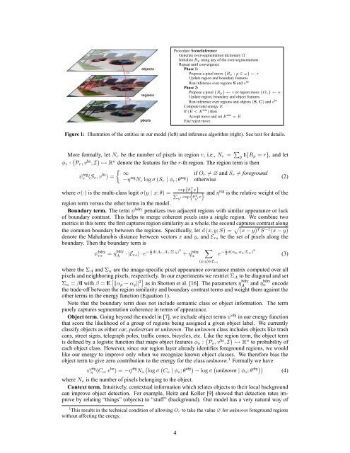
Procedure SceneInference
Generate over-segmentation dictionary Ω
Initialize Rp using any of the over-segmentations
Repeat until convergence
Phase 1:
Propose a pixel move {Rp : p ∈ ω} ← r
Update region and boundary features
Run inference over regions S and v hz
Phase 2:
Propose a pixel {Rp} ← r or region move {Or} ← o
Update region, boundary and object features
Run inference over regions and objects (S,C) and v hz
Compute total energy E
If (E < E min ) then
Accept move and set E min = E
Else reject move
Figure 1: Illustration of the entities in our model (left) and inference algorithm (right). See text for details.
More formally, let Nr be the number of pixels in region r, i.e., Nr =
p 1{Rp = r}, and let
φr : Pr,v hz , I ↦→ R n denote the features for the r-th region. The region term is then
ψ reg
r (Sr,v hz ) =
∞ if Or = ∅ and Sr = foreground
−η reg Nr log σ (Sr | φr;θ reg ) otherwise
where σ(·) is the multi-class logit σ(y | x;θ) = exp{θT y x}
n
P
y
′ exp
θ T
y ′x
(2)
o and η reg is the relative weight of the
region term versus the other terms in the model.
Boundary term. The term ψ bdry penalizes two adjacent regions with similar appearance or lack
of boundary contrast. This helps to merge coherent pixels into a single region. We combine two
metrics in this term: the first captures region similarity as a whole, the second captures contrast along
the common boundary between the regions. Specifically, let d (x,y;S) = (x − y) T S −1 (x − y)
denote the Mahalanobis distance between vectors x and y, and Ers be the set of pixels along the
boundary. Then the boundary term is
ψ bdry
rs = η bdry
A · |Ers|
1 −
· e 2 d(Ar,As;ΣA)2
+ η bdry
α
(p,q)∈Ers
1 −
e 2 d(αp,αq;Σα)2
where the ΣA and Σα are the image-specific pixel appearance covariance matrix computed over all
pixels and neighboring pixels, respectively. In our experiments we restrict ΣA to be diagonal and set
Σα = βI with β = E αp − αq2 as in Shotton et al. [16]. The parameters η bdry
A and ηbdry α encode
the trade-off between the region similarity and boundary contrast terms and weight them against the
other terms in the energy function (Equation 1).
Note that the boundary term does not include semantic class or object information. The term
purely captures segmentation coherence in terms of appearance.
Object term. Going beyond the model in [7], we include object terms ψobj in our energy function
that score the likelihood of a group of regions being assigned a given object label. We currently
classify objects as either car, pedestrian or unknown. The unknown class includes objects like trash
cans, street signs, telegraph poles, traffic cones, bicycles, etc. Like the region term, the object term
is defined by a logistic function that maps object features φo : Po,v hz , I ↦→ Rn to probability of
each object class. However, since our region layer already identifies foreground regions, we would
like our energy to improve only when we recognize known object classes. We therefore bias the
object term to give zero contribution to the energy for the class unknown. 1 Formally we have
ψ obj
n (Co,v hz ) = −η obj
No log σ Co | φo;θ obj − log σ unknown | φo;θ obj
(4)
where No is the number of pixels belonging to the object.
Context term. Intuitively, contextual information which relates objects to their local background
can improve object detection. For example, Heitz and Koller [9] showed that detection rates improve
by relating “things” (objects) to “stuff” (background). Our model has a very natural way of
1 This results in the technical condition of allowing Or to take the value ∅ for unknown foreground regions
without affecting the energy.
4
(3)