Heart rate (residual) - Stanford University
Heart rate (residual) - Stanford University
Heart rate (residual) - Stanford University

You also want an ePaper? Increase the reach of your titles
YUMPU automatically turns print PDFs into web optimized ePapers that Google loves.
Frequency of words<br />
Frequency of words<br />
1st and 2nd This paper proposes a nonparametric Bayesian method for exploratory data analysis<br />
day<br />
and<br />
after<br />
feature<br />
birth<br />
construction in continuous time series. Our method focuses on<br />
understanding shared features in a set of time series that exhibit significant individual<br />
variability. Our method builds on the framework of latent Diricihlet allocation<br />
(LDA) and its extension to hierarchical Dirichlet processes, which allows us<br />
to characterize each series as switching between latent “topics”, where each topic<br />
is characterized as a distribution over “words” that specify the series dynamics.<br />
However, unlike standard applications of LDA, we discover the words as we learn<br />
the model. We apply this model to the task of tracking the physiological signals<br />
of premature infants; our model obtains clinically significant insights as well as<br />
useful features for supervised learning tasks.<br />
7th and 8th Time series data is ubiquitous. The task of knowledge discovery from such data is useful in many scientific<br />
disciplines … dincluding understanding ddisease (b)<br />
…pathogenesis<br />
from longitudinal studies, mining<br />
social interactions, and t wildlife monitoring. t+1 Dynamic models that can succinctly capture generation<br />
of measured day data after as birth a function of underlying latent states can serve as a lens into understanding<br />
series structure. For example, generation of physiologic data by latent disease states can help reveal<br />
how the set of diseases manifest and uncover novel disease associations.<br />
(a) (c)<br />
(d)<br />
g n<br />
1 Introduction<br />
d<br />
g l<br />
k<br />
k<br />
Discovering shared and individual latent structure in<br />
multiple time series<br />
D<br />
Suchi Saria 1 , Daphne Koller 1 and Anna Penn 2<br />
1 Department of Computer Science, 2 Department of Pediatrics<br />
<strong>Stanford</strong> <strong>University</strong><br />
<strong>Stanford</strong>, CA 94305<br />
ssaria@cs.stanford.edu<br />
o t+1<br />
… yt y t+1<br />
Abstract<br />
Traditional generative models for time series data (such as switching Kalman filters[1]) do not explicitly<br />
model generation of a continuum of heterogeneous exemplar series. However, in the domain<br />
of modeling disease physiology, the set of clinical diagnoses for most diseases is not naturally discrete;<br />
patients suffer from diseases to varying extents, and even within disease labels, patients exhibit<br />
significant variability. Furthermore, often the diagnosis is the result of a clinical observation with<br />
significant uncertainty regarding both the onset and the nature of the disease. Increasing representation<br />
granularity by increasing the number of classes can help, but ad hoc discretization into a fixed<br />
set limits our ability to model instance-specific variability. Moreover, the combinatorics quickly get<br />
out of hand when one considers combinations of different diseases, a situation that is unfortunately<br />
quite common in practice.<br />
In the domain of natural language processing, topic models have found great success as a representation<br />
for uncovering the underlying structure of document corpora [2, 7]. A document is associated<br />
with a distribution over latent variables called zt z topics, each of which defines a distribution over words.<br />
At a high level, this paradigm <strong>Heart</strong> extends <strong>rate</strong> (<strong>residual</strong>) naturally t+1tosignal<br />
applications such as disease modeling: individual<br />
patients maintain their own distributions over disease topics, so each patient can be expressed as<br />
a point lying in the continuous disease (topic) simplex. Each topic defines a distribution over dynamic<br />
behaviors observed in the time series. These dynamic behaviors, play the role of “words” in<br />
1<br />
…<br />
N
this framework; these words are shared across topics, allowing us to uncover relationships between<br />
different disease states.<br />
To construct this approach, we build on the framework of hierarchical Dirichlet processes, which<br />
was designed to allow sharing of mixture components within a multi-level hierarchy. While conceptually<br />
straightforward, this extension involves some significant subtleties. Most obviously, current<br />
implementations of topic models assume that the expressed features are pre-specified and only the<br />
latent topic variables are inferred. To apply this framework to continuous data such as physiologic<br />
time series, we must define a notion of a “word”. Loosely speaking, a word specifies the parameterization<br />
of the function that gene<strong>rate</strong>s the system dynamics for the duration of the word. Moreover,<br />
the duration of the word is also not fixed in advance, and may vary from one occurrence to the next.<br />
Hence, our representation of a time series in terms of words must also postulate word boundaries.<br />
In the remainder of this paper, we define our generative time series topic model (TSTM), and provide<br />
an efficient block Gibbs sampling scheme for performing full Bayesian inference over the model.<br />
We then present results on our target application of analyzing physiological time series data, demonstrating<br />
its usefulness both for analyzing the behavior of different time series, and for constructing<br />
features that are subsequently useful in a supervised learning task.<br />
2 Related Work<br />
An enormous body of work has been devoted to the task of modeling time series data. Probabilistic<br />
generative models, the category to which our work belongs, typically utilize a variant of a switching<br />
dynamical system [1], where one or more discrete state variables determine the momentary system<br />
dynamics, which can be either linear or in a richer parametric class. However, these methods typically<br />
utilize a single model for all the time series in the data set, or at most define a mixture over<br />
such models, using a limited set of classes. These methods are therefore unable to capture significant<br />
individual variations in the dynamics of the trajectories for different patients, as required in our data.<br />
Recent work by Fox and colleagues [5, 3, 4] uses nonparametric Bayesian models for capturing<br />
generation of continuous-valued time series. Conceptually, the present work is most closely related<br />
to BP-AR-HMMs [5], which use Beta processes to share observation models, characterized by autoregressive<br />
processes (AR), across series. Thus, it captures variability between series by sampling<br />
subsets of low-level features that are specific to individual series. However, BP-AR-HMMs are<br />
aimed at capturing individual variation that manifests as words (features) that are unique to a particular<br />
time series. By comparison, we aim to capture higher-level concepts that occur broadly across a<br />
subpopulation (e.g., physiologic characteristics exhibited by Lung disorders) while modeling seriesspecific<br />
variability in terms of the extent to which these higher-level concepts are expressed (e.g.,<br />
transient respiratory disorder versus long term respirator distress). Other works [3, 4] have utilized<br />
hierarchical Dirichlet process priors for inferring the number of features in hidden Markov models<br />
and switching linear dynamical systems, but these models do not try to represent variability across<br />
exemplar series. Temporal extensions of LDA [19, 20] model evolution of topic compositions over<br />
time in text data but not continuous-valued temporal data.<br />
A very different approach to analyzing time series data is to attempt to extract meaningful features<br />
from the trajectory without necessarily constructing a generative model. For example, one standard<br />
procedure is to re-encode the time series using a Fourier or wavelet basis, and then look for large<br />
coefficients in this representation. However, the resulting coefficients do not capture signals that are<br />
meaningful in the space of the original signal, and are therefore hard to interpret. Features can also<br />
be constructed using alternative methods that produce more interpretable output, such as the work<br />
on sparse bases [11]. However, this class of methods, as well as others [13], require that we first<br />
select a window length for identifying common features, whereas no such natural granularity exists<br />
in many applications. Moreover, none of these methods aim to discover higher level structure where<br />
words are associated with different “topics” to different extents.<br />
Our specific domain of neonatal monitoring has been previously studied in a machine learning setting<br />
[21, 14], but focusing on the different task of monitoring for known events (e.g., sensor drops).<br />
2
3 Time Series Topic Model<br />
Time Series Topic Model (TSTM) is an extension of Latent Dirichlet Allocation (LDA) [2] for<br />
time-series data. Latent Dirichlet Allocation (LDA) is a generative probabilistic model for text<br />
corpora. It makes the assumption that there is an underlying fixed set of topics that is common to the<br />
heterogeneous collection of documents in the corpus. A topic is a distribution over the vocabulary<br />
of all words present in the corpus. A document is gene<strong>rate</strong>d by first choosing a document-specific<br />
mixing proportion over the topics. To sample each word, sample a topic, and then sample a word<br />
from that topics’ distribution over words.<br />
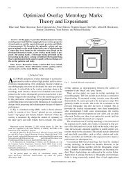
Unlike text, in time series data often the features to be extracted are structurally not obvious (see<br />
figure 2). Pre-segmenting the sequence data into “words” does not offer sufficient flexibility to<br />
learn from the data, especially in the realm of exploration for knowledge discovery. Thus, we<br />
integ<strong>rate</strong> feature discovery into a temporal extension of LDA. We describe below each of the TSTM<br />
components (in a bottom-up fashion).<br />
Data generation model: We assume that the continuous-valued data yt at time t is gene<strong>rate</strong>d using<br />
a function fk from a finite set F of generating functions. These functions take as inputs xt, values<br />
dependent on current and previous time slices, and gene<strong>rate</strong> the output as yt = fk(xt; θk). fk, an<br />
expressive characterization of the time series dynamics, can be thought of as th kth word in the timeseries<br />
corpus vocabulary. Hereafter, we use words and generating functions interchangeably. The<br />
parameterization of fk depends on the choice of the observation model. We choose to use vector<br />
autoregressive processes, which are used for temporal modeling in numerous domains, including<br />
medical time series of fMRI and EEG. Other observation models (such as an SLDS with mixture<br />
model emissions [3]) can also be used.<br />
In an order p autoregressive process, given a function fk with<br />
parameters {A k , V k }, the observation is gene<strong>rate</strong>d as:<br />
yt = A k X T t + vt vt ∼ N(0, V k ) (1)<br />
where yt ∈ Rm×1 for an m-dimensional series. The inputs<br />
Xt = [yt−1, . . . ,yt−p]. Parameters Ak ∈ Rm×p , and V k is<br />
an m × m positive-semidefinite covariance matrix. The kth<br />
word then corresponds to a specific instantiation of the generating<br />
function parameters {Ak , V k }. For TSTM, we want the<br />
words to persist for more than one time-step. Thus, for each<br />
word, we have an additional parameter ωk that specifies mean<br />
length of the word as 1/ωk. Our goal now is to uncover this D<br />
set of functions F, via instantiations of the generating function<br />
parameters, denoted more generally as θk ∈ Θ.<br />
N d<br />
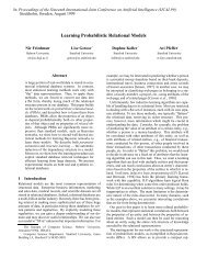
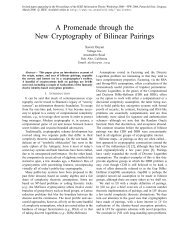
(b) HDP mixture model<br />
g l<br />
g<br />
k<br />
d<br />
D<br />
k<br />
…<br />
n<br />
d t<br />
z t<br />
o t+1<br />
d t+1<br />
z t+1<br />
…<br />
…<br />
yt yt+1 …<br />
N<br />
(c) Time Series Topic Model<br />
Figure 1: Graphical representation<br />
of the time series topic model<br />
Word and Topic descriptions: To uncover the finite generating function set F, such that these<br />
functions are shared across latent topics, we use the hierarchical Dirichlet process[18] (HDP). A<br />
Dirichlet process (DP), denoted by DP(γ, H), yields a distribution on discrete measures. H is a base<br />
(continuous or discrete) probability measure on Θ and γ is the concentration parameter. Sethuraman<br />
[17] shows that G0 ∼ DP(γ, H), a sample drawn from the DP, is a discrete distribution because,<br />
with probability one:<br />
k−1 <br />
G0 = Σ ∞ k=1βkδθk θk ∼ H βk = β ′ k (1 − β<br />
l=1<br />
′ l ) β′ k<br />
∼ Beta(1, γ) (2)<br />
Draws from H yield the location of “sticks”’, δθk , in the discrete distribution. The generation of the<br />
stick weights βk is denoted by β ∼ GEM(γ). Thus, we use the DP to place priors on the mixture<br />
of generating functions by associating a generating function with each stick in G0. In addition, by<br />
associating each data sample (time point in a series) with a specific generating function via indicator<br />
variables, the posterior distribution yields a probability distribution on different partitions of the data.<br />
The mixing proportion (the stick weights) in the posterior distribution are obtained from aggregating<br />
corresponding weights from the prior and the assigned data samples.<br />
HDPs [18] extend the DP to enable sharing of generating functions between topics. If discrete measures<br />
Gj are sampled with the discrete measure G0 as its base measure, the resulting distributions<br />
3
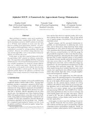
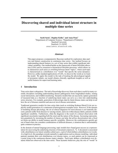
<strong>Heart</strong> <strong>rate</strong> (<strong>residual</strong>) signal<br />
Figure 2: <strong>Heart</strong> signal (mean removed) from three infants in their first few hours of life<br />
have non-zero probability of regenerating the same sticks, thereby sharing generating functions between<br />
related topics. Thus, a draw Gj from the HDP with G0 as its base measure, Gd ∼ DP(η, Go),<br />
can be described as:<br />
Gd = Σ ∞ k=1 φdkδθk φd ∼ DP(η, β), β ∼ GEM(γ), θk ∼ H (3)<br />
where φd represents the topic specific mixing proportions over the generating functions and β represents<br />
the global mixing proportion. Similar to [5], we use a matrix-normal inverse-Wishart on the<br />
parameters {A k , V k } and a symmetric Beta prior on ωk as our base measures H.<br />
Dynamics of words and topics: Given the words F, topics φ1:D and series-specific transition<br />
matrices πn, the series generation is straightforward. For each time slice t ∈ 1, · · ·,T , we gene<strong>rate</strong>:<br />
1. Current latent topic state given topic at previous time-step, dt ∼ Mult(π dt−1<br />
n )<br />
2. Switching variables ot, which determine whether a new word is selected. A new word<br />
is always gene<strong>rate</strong>d (ot = 0) if the latent state has changed from the previous time step;<br />
otherwise, ot is selected from a Bernoulli distribution whose parameter determines the<br />
word length. Thus, ot ∼ I(dt = dt−1)Bernoulli(ωzt−1), where I is the indicator function.<br />
3. The identity of the generating function (word) to be applied; if ot = 1, we have zt = zt−1,<br />
otherwise zt ∼ Mult(φdt).<br />
4. Observation given the generating function index zt as yt ∼ fzt(xt−1; θzt).<br />
The-series specific topic transition distribution πn is gene<strong>rate</strong>d from the global topic transition distribution<br />
πg. Hyperparameters αl controls the degree of sharing across series in our belief about the<br />
prevalence of latent topic states. A large αl assigns a stronger prior and allows less variability across<br />
series. To gene<strong>rate</strong> πn, each row i is gene<strong>rate</strong>d from Dir(αlπi g ), where πi g is the ith row of the global<br />
topic transition distribution. Given hyperparameters, αg and κ, πi g ∼ Dir(αg + κδi). κ controls the<br />
degree of self-transitions for the individual topics.<br />
4 Approximate Inference using block-Gibbs<br />
Several approximate inference algorithms have been developed for mixture modeling using the<br />
HDP; see [18, 3, 10] for a discussion and comparison. We use a block-Gibbs sampler that relies<br />
on the degree L weak limit approximation presented in [8]. This sampler has the dvantage of being<br />
simple, computationally efficient and shows faster mixing than most alternate sampling schemes [3].<br />
The block-Gibbs sampler for TSTM proceeds by alternating between sampling of the state variables<br />
{dt, zt}, the model parameters, and the series specific transition matrices. To introduce notation<br />
briefly, we use 1 : T to mean all indices 1 through T . n indexes individual series. We drop subindices<br />
when all instances of a variable are used (for e.g., z1:N,1:Tn is written as z for short). We<br />
drop the index n when explicit that that the variable refers to a single series. We detail the update<br />
steps of our block-Gibbs inference algorithm below.<br />
Sampling latent topic descriptions β, φd: The DP can also be viewed as the infinite limit of the<br />
order L mixture model [8, 18]:<br />
β|γ ∼ Dirichlet(γ/L, · · ·,γ/L) φd ∼ Dirichlet(ηβ) θk ∼ H (4)<br />
We can approximate the limit by choosing L to be larger than the expected number of words in the<br />
data set. The prior distribution over each topic-specific word distribution is then:<br />
φd|β, η ∼ Dir(ηβ1, · · · , ηβL) (5)<br />
4
Within an iteration of the sampler, let md,l be the counts for the number of times zn,t sampled<br />
the lth word1 for the dth disease topic; that is, let md,l = <br />
n=1:N t=1:Tn I(zn,t = l)I(dn,t =<br />
d)I(on,t = 0) and m.,l = <br />
d=1:D md,l. The posterior distribution for the global and individual<br />
topic parameters is:<br />
β|z, d, γ ∼ Dir(γ/L + m.,1, · · ·,γ/L + m.,L) (6)<br />
φd ′|z, d, η, β ∼ Dir(ηβ1 + md ′ ,1, · · ·,ηβL + md ′ ,L) (7)<br />
Sampling word parameters ωl and θl: Loosely, the mean word length of the lth word is 1/ωl.<br />
A symmetric Beta prior with hyperparameter ρ, conjugate to the Bernoulli distribution, is used as<br />
a prior over word lengths. The sufficient statistics needed for the posterior distribution of ωl are<br />
the counts ¯cl,i = <br />
n=1:N t=1:Tn I(dn,t = dn,t−1)I(zn,t−1 = l)I(on,t = i) where i ∈ {0, 1},<br />
representing the number of time steps, across all sequences, in which the topic remained the same,<br />
the word was initially l, and the word either changed (on,t = 1) or not (on,t = 0). Thus,<br />
ωl|¯cl,., ρ ∼ Beta(ρ/2 + ¯cl,1, ρ/2 + ¯cl,0) (8)<br />
For sampling the AR generating function parameters, note that conditioned on the mode assignments<br />
z, the observations y1:T,1:N can be partitioned into sets corresponding to each unique l ∈ L. This<br />
gives rise to L independent linear regression problems of the form Y l = A l X l +E l where Y l is the<br />
target variable, with observations gene<strong>rate</strong>d from mode l, stacked column-wise. X l is a matrix with<br />
the corresponding r lagged observations and E l is the corresponding noise matrix. The parameters<br />
A l and V l are sampled from the posterior given conjugate priors of the Matrix-Normal Inverse-<br />
Wishart, similar to [5].<br />
Sampling global and series-specific transition matrices, πg and πn: Since the number of topic<br />
states D is known, and we use conjugate priors of Dirichlet distribution for each row of the transition<br />
matrix, the posterior update simply involves summing up counts from the prior and the data. The relevant<br />
count vectors are computed as ci n,k = Tn t=1 I(dn,t−1 = i)I(dn,t = k) and ci k = N n=1 ci n,k<br />
which aggregates over each series. ci = {ci 1, · · ·,c i D } and i indexes a row of the transition matrix:<br />
π i g|d, αg, κ ∼ Dir(αg + κδi + c i ) π i n|πg, d, αl ∼ Dir(αlπ i g + c i n,1:D) (9)<br />
Sampling state variables: If all model parameters (topic and word descriptions) are specified,<br />
then one can exploit the structure of the dependency graph to compute the posterior over the state<br />
variables using a single forward-backward pass. This is the key motivation behind using block<br />
Gibbs. The joint posterior can be computed recursively. Forward sampling is used to sample the<br />
variables in each time slice given samples for the previous time slice:<br />
P(z1:T,d1:T |y1:T,π) = <br />
P(zt, dt|zt−1, dt−1, y1:T,π) (10)<br />
Top-down sampling is used within a given time slice. See appendix A for details.<br />
5 Experiments and Results<br />
t<br />
We demonst<strong>rate</strong> the utility of TSTM on physiologic heart <strong>rate</strong> (HR) signal collected from premature<br />
infants of gestational age ≤ 34 weeks and birth weight ≤ 2000 grams admitted to the XXX<br />
(anonymized) neonatal ICU within the first few hours of life. Our inclusion criteria resulted in data<br />
from 145 infants. 2 These infants are continuously monitored as part of routine care and data aggregated<br />
at the minute-level granularity was stored. These infants are extremely vulnerable, and<br />
complications during their stay in the NICU can adversely affect long term neurological development.<br />
Clinicians and alert systems implemented on ICU monitors utilize coarse information based<br />
on thresholding of the signal mean (e.g., HR > 160 bpm) and discard the dynamics as noise. We<br />
use TSTM to discover whether there is information contained in the signal dynamics. As infants<br />
1 Within this approximation, words get re-ordered such that all words that are observed in the corpus are<br />
assigned indices less than L. Thus, l indexes the lth observed word which can correspond to different parameter<br />
instantiations over different iterations.<br />
2 All work was performed under protocol 8312 approved by XXX’s (anonymized) Panel on Human Subjects.<br />
5
mature, they become less vulnerable; their base heart <strong>rate</strong> also lowers. We preprocess the signal to<br />
remove the basal signal computed from taking a 40 minute moving average window. Removing the<br />
base signal allows us to capture characteristics only related to the dynamics of the signal (see raw<br />
signal in figure 2).<br />
Partially-supervised training: We first experimented with a partially-supervised training regime of<br />
labeled LDA [15], where during training, we constrain infant-specific transition matrices not to have<br />
topics corresponding to complications that they did not show symptoms for. This form of training<br />
has the advantage of biasing the topics into categories that are coherent and more easily interpreted.<br />
We define four broad clinically meaningful topics: Lung for primarily lung related complications<br />
such as RDS; Hemorrhage for head related complications such as IVH; Multi as the catch-all class<br />
for severe complications that often affect multiple organ systems; and Healthy.<br />
For each infant in a randomly chosen subset of 30 infants, we assign a vector λn of length D = 4,<br />
where we have a 0 at index i when this infant is known not to have complications related to the ith<br />
category. All infants are marked to have the healthy topic, representing the assumption that there is<br />
some fraction of their time in the NICU at which they exhibit behaviors of a healthy baby.<br />
Each row of the infant-specific transition matrix is gene<strong>rate</strong>d as:<br />
<br />
π i n<br />
∼ Dir<br />
π<br />
αl<br />
i g ⊗ λn<br />
< πi g, λn ><br />
λn(i) = 1 (11)<br />
where ⊗ denotes the element-wise vector product. We used an AR(1) process as our observation<br />
model and set the L to 15. We experimented with a few different settings of the hyperparameters;<br />
upon visual inspection, the relative distribution of words for each infant looked similar. For the<br />
reported experiments, αl, γ and η were each set to 10, κ = 25 and ρ = 20. We run 2000 iterations<br />
for each Gibbs chain.<br />
Qualitative evaluation: We fix the topic distributions φ1:D to that of the 2000th Gibbs iteration and<br />
run inference on our larger set of 145 infants. Here, no supervision is given; that is, both πg and πn<br />
are initialized from the prior and are left unconstrained during the inference process (using block<br />
Gibbs). We ran three sepa<strong>rate</strong> Gibbs chains to 400 iterations. Given the topics, the block-Gibbs<br />
sampler appears to mix within 200 iterations.<br />
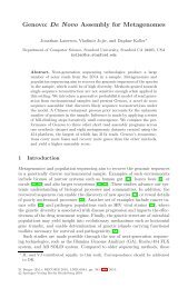
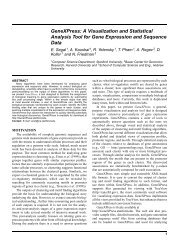
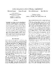
In figure 3, we analyze 30 randomly selected infants from this test set at the 400th iteration from<br />
chain 1. In panel (a), we plot the word distribution for days 1,2 (top) and days 7,8 (bottom). Several<br />
interesting observations arise: the infants follow a continuum of word distribution profiles. Infants<br />
with no complications, shown as red squares at the bottom of panel (a), express words 3, 9 and 10<br />
in much greater proportion than the other infants. As can be seen in (b), these words are primarily<br />
associated with the Healthy topic. Figure 3d shows examples of words extracted from the data. The<br />
words with the highest mutual information with the Healthy topic appear to have higher frequencies.<br />
Words with AR parameter a > 1 generally represent heart <strong>rate</strong> accelerations (e.g., word 8 shown in<br />
gray); words where a is positive and close to 0 represent periods with significantly lower dynamic<br />
range (e.g., word 2 shown in purple). Thus, our model seems to imply a correlation between the<br />
health of the infant and the extent to which their heart <strong>rate</strong> exhibits significant variations.<br />
Respiratory distress (RDS), a common complication of prematurity, usually resolves within the first<br />
few days as the infant stabilizes and is transitioned to room air. This is reflected by the decrease in<br />
relative proportion of word 2, only associated with the Lung topic. Exceptions to this are infants 3<br />
and 30, both of whom have chronic lung problems.<br />
To demonst<strong>rate</strong> the insights provided by this representation, we examine the clinical evolution of<br />
three sample infants — 2, 16 and 23 — chosen to be illustrative of different trajectories of the<br />
word distributions. In figure 3c, we show the posterior for the Healthy topic being expressed from<br />
averaging over 30 Gibbs chains. The bold line shows the smoothed posterior over time. Infant 2 (I2)<br />
was born with a heart defect called VSD (can be acutely life-threatening) and a mode<strong>rate</strong> size patent<br />
ductus arteriosus (PDA), both of which cause left to right shunting and disrupt blood flow to the<br />
body. I2 was ligated on day 4, a procedure performed to resolve PDA. She was also on dopamine<br />
starting day 2 due to hypotension, had a renal failure on day 3 post indomethacine (medication<br />
for PDA) and was on a ventilator during this entire time. On Day 7, her state started to resolve<br />
significantly, and on day 8 her ventilator settings were minimal and she was taken off dopamine. Her<br />
empirical evolution closely tracks her medical history; in particular, her state continually improves<br />
6
Frequency of words<br />
Frequency of words<br />
1 st and 2 nd day after birth<br />
7 th and 8 th day after birth<br />
(a) (c)<br />
(d)<br />
Figure 3: (a) Inferred word distributions for 30 infants during their stay at the NICU, (b) distribution<br />
over disease topic given words for the population, (c) inferred posterior (and smoothed version<br />
shown in bold) over latent state, Healthy, (d) examples of inferred features extracted from the data.<br />
after day 4. Infant 16 was a healthier preemie with few complications of prematurity and was<br />
discharged on day 4. Infant 23, on the other hand, got progressively sicker and eventually died on<br />
day 4. The figure shows that their inferred posterior prediction closely tracks their medical history<br />
as well. Of note, the ventilator controls only oxygen supply and does not directly control the heart<br />
<strong>rate</strong>, so the inferred topics are not just uncovering the different ventilator settings.<br />
Quantitative evaluation: To provide a more quantitative evaluation, we extract grades G1:N that<br />
represent an infant’s health based on his final outcome, as identified retrospectively by a clinician.<br />
Grade 0 represents no complications; grade 1 to isolated minor complications frequently associated<br />
with prematurity; grade 2 to multiple minor complications; grade 3 to major complications at low<br />
grade; and grade 5 to major complications at severe grades. We defined a “health ranking” H over<br />
infants, based on their relative frequency of the Healthy topic. The rank score for a ranking H is:<br />
(b)<br />
rankscoreH = Σ N n=1 ΣN m=1 I(H(n) > H(m))(Gn − Gm) (12)<br />
The maximal achievable score for our dataset is 22992 for the perfect ordering while a random ordering<br />
has an expected score of 0. For comparison, we compute the rank score from SNAP [16], a<br />
validated and highly accu<strong>rate</strong> score that characterizes illness severity based on birth characteristics,<br />
laboratory tests and monitor data at 12 hours of life. SNAP achieves a score of 13030, corresponding<br />
to 78.3% of the overall range. Based on dynamics alone, TSTM (in the median from three<br />
Gibbs trials) achieves a score of 10432 corresponding to 72.69% at the first 12 hours and 11314<br />
corresponding to 74.6% from the first 8 days. Although SNAP achieves a slightly higher score, it<br />
incorpo<strong>rate</strong>s multiple biomarkers including invasive tests.<br />
Comparison to Fourier features: The preceding analysis ranked babies using only a single feature<br />
extracted from the TSTM model — the frequency of the Healthy topic. To test whether informa-<br />
7
tion is present in the entire topic distribution, we use a supervised learning regime where we train<br />
a support vector machine with a ranking objective [9] to predict the infant’s disease grade. In this<br />
supervised setting, we wanted to compare to features constructed by the fast Fourier transform,<br />
a commonly used feature processing scheme for time-series data. The FFT seems appropriate in<br />
this setting, since we observed earlier that words associated with the Healthy topic tend to exhibit<br />
higher frequencies. The frequencies of the resulting FFT coefficients span 1/v for v ∈ {1, · · ·,T }.<br />
Based on preliminary data analysis, we compute FFT features from a grid of periods between 4<br />
and 40 minutes in increments of 4 minutes. We use each of the FFT coefficients as a feature in the<br />
ranking SVM. To make for a fairer comparison, we estimate the parameters of TSTM without any<br />
supervision, using 6 topics; we use the proportions for each of the 6 topics as features of the time<br />
series in the ranking SVM. 3 . We report results averaged over 20 random folds with 50–50 train/test<br />
splits. The SVM tradeoff parameter C was set using cross-validation. SVM TSTM and SVM FFT<br />
achieve mean performance (relative to maximum rank for each split) of 72.74% and 63.5% respectively<br />
(with a random order having a mean score of 50.0%). This suggests that the inferred topic<br />
distributions provide a useful feature representation scheme that can be employed within supervised<br />
objectives as an alternative or in addition to the FFT.<br />
Comparison to BP-AR-HMM: As discussed in section 2, BP-AR-HMMs is the generative model<br />
for time series data that is most closely related to our work. For a visual comparison of the difference<br />
between TSTM and BP-AR-HMM, we used the BP-AR-HMM to infer word distributions over the<br />
same 30 infants shown in figure 3a. Since BP-AR-HMM is sampling in the space of binary matrices,<br />
it takes much longer to mix. Thus, due to computational resource constraints, we were only able to<br />
run BP-AR-HMMs on the first four days of data.<br />
We experimented with different values of the parameters, but found that the model generally tends<br />
to encourage the generation of multiple unique, series-specific features (see example figure in supplementary<br />
materials). This behavior is not surprising, since the notion of individual series variation<br />
in BP-AR-HMMs is quite different from that in TSTMs: TSTMs, like topic models, encourage<br />
sharing by having all series utilize the same set of topics, but to different extents; by contrast, BP-<br />
AR-HMMs have some features that are shared and others that are explicitly series-specific. Thus,<br />
the two models are likely to be useful for fairly different types of exploratory data analysis.<br />
We also performed a quantitative comparison regarding the utility of these features for a supervised<br />
learning task. We trained an SVM classifier, using leave-one-out cross-validation, to distinguish<br />
Healthy vs Not healthy, using the labels shown at the bottom of figure 3a. We compared the features<br />
derived from BP-AR-HMM from those inferred in an unsupervised manner using TSTM for a 4<br />
topic model. The SVM using the 4 features learned by TSTM has an accuracy of 80% while the<br />
SVM using the 43 features inferred by BP-AR-HMM has an accuracy of 70%. Again, this is not<br />
surprising, since the fragmentation of the data across multiple individual features is bound to hurt<br />
performance, especially for such a small data set.<br />
6 Discussion and Future work<br />
In summary, the primary contribution of this paper is a new class of models for time-series data<br />
that emphasizes the modeling of instance specific variability while discovering population level<br />
characteristics. We demonst<strong>rate</strong> its use in a novel and useful application of modeling heterogeneous<br />
patient populations over time. Towards this end, we extended the existing topic modeling framework<br />
to also simultaneously discover the finite set of features (words) expressed in the data. We believe<br />
that TSTM provides a significant departure from current practices and a flexible tool for exploratory<br />
time series data analysis in novel domains. Furthermore, learned topic or word distributions can<br />
serve as features within supervised tasks. We demonst<strong>rate</strong>d the utility of TSTMs on medical time<br />
series, but the framework is broadly applicable to other time-series applications.<br />
Clinically, our work independently validates existing knowledge about heart <strong>rate</strong> dynamics containing<br />
information for characterizing health of a fetus [22] and predicting infection and death near<br />
onset time in premature infants[6]; furthermore, it suggests that information contained in the dynamics<br />
might be informative for a broader set of complications than infection and death.<br />
3 Due to the size of our corpus, the topic descriptions were inferred from only 30% of the data and fixed at<br />
the 2000th iteration. Thereafter, we infer series-specific topic proportions based on these fixed settings of the<br />
model parameters.<br />
8
Several extensions of LDA that model additional structure in the data [19, 20, 12] can add to the<br />
expressiveness of TSTMs. In particular, modeling disease composition over time (analogous to<br />
[19]) and disease evolution within a single patient (analogous to [20]) should provide interesting<br />
insight. We leave these next steps for future work.<br />
References<br />
[1] Y. Bar-Shalom and T. E. Fortmann. Tracking and Data Association. Academic Press Professional,<br />
Inc., 1987.<br />
[2] D. Blei, A. Ng, and M. Jordan. Latent Dirichlet allocation. In J. Mach. Learn. Res. 2003.<br />
[3] E. Fox, E. Sudderth, M. Jordan, and A. Willsky. The sticky HDP-HMM: Bayesian nonparametric<br />
hidden Markov models with persistent states. Technical Report P-2777, MIT LIDS,<br />
2007.<br />
[4] E. Fox, E. Sudderth, M. Jordan, and A. Willsky. Nonparametric Bayesian learning of switching<br />
linear dynamical systems. In NIPS. 2008.<br />
[5] E. Fox, E. Sudderth, M. Jordan, and A. Willsky. Sharing features among dynamical systems<br />
with Beta Processes. In NIPS. 2009.<br />
[6] M. Griffin, D. Lake, E. Bissonette, F. Harrell, T. O’Shea, and J. Moorman. <strong>Heart</strong> <strong>rate</strong> characteristics:<br />
novel physiomarkers to predict neonatal infection and death. In Pediatrics. 2005.<br />
[7] T. Griffiths and M. Steyvers. Finding scientific topics. In PNAS. 2004.<br />
[8] H. Ishwaran and M. Zarepour. Exact and approximate sum-representation for the Dirichlet<br />
process. In Canadian Journal of Statistics. 2002.<br />
[9] T. Joachims. Training linear SVMs in linear time. In KDD. 2006.<br />
[10] K. Kurihara, M. Welling, and Y. W. Teh. Collapsed variational Dirichlet process mixture<br />
models. In IJCAI, 2007.<br />
[11] H. Lee, Y. Largman, P. Pham, and A. Ng. Unsupervised feature learning for audio classification<br />
using convolutional deep belief networks. In NIPS, 2009.<br />
[12] W. Li and A. McCallum. Pachinko Allocation: DAG-structured mixture models of topic correlations.<br />
In ICML, 2006.<br />
[13] A. Mueen, E. Keogh, Q. Zhu, S. Cash, and B. Westover. Exact discovery of time series motifs.<br />
In SDM, 2009.<br />
[14] J. Quinn, C. Williams, and N. McIntosh. Factorial switching linear dynamical systems applied<br />
to physiological condition monitoring. In IEEE Trans. Pattern Analysis Machine Intelligence,<br />
2009.<br />
[15] D. Ramage, D. Hall, R. Nallapati, and C. Manning. Labeled LDA: A supervised topic model<br />
for credit attribution in multi-labeled corpora. In EMNLP, 2009.<br />
[16] D. Richardson, J. Gray, M. McCormick, K. Workman, and D. Goldmann. Score for neonatal<br />
acute physiology: a physiologic severity index for neonatal intensive care. In Pediatrics. 1993.<br />
[17] J. Sethuraman. A constructive definition of Dirichlet priors. In Statistics Sinica. 1994.<br />
[18] Y. W. Teh, M. Jordan, M. Beal, and D. Blei. Hierarchical Dirichlet processes. In JASA. 2006.<br />
[19] C. Wang, D. Blei, and D. Heckerman. Continuous time dynamic topic models. In UAI. 2008.<br />
[20] X. Wang and A. McCallum. Topics over Time: A non-Markov continuous time model of<br />
topical trends. In KDD, 2006.<br />
[21] C. Williams, J. Quinn, and N. McIntosh. Factorial switching Kalman filters for condition<br />
monitoring in neonatal intensive care. In NIPS, 2005.<br />
[22] K. Williams and F. Galerneau. Intrapartum fetal heart <strong>rate</strong> patterns in the prediction of neonatal<br />
acidemia. In Am J Obstet Gynecol. 2003.<br />
9