Cause and Extend of the Extreme Radio Flux Density
Cause and Extend of the Extreme Radio Flux Density
Cause and Extend of the Extreme Radio Flux Density

Create successful ePaper yourself
Turn your PDF publications into a flip-book with our unique Google optimized e-Paper software.
CAUSE AND EXTENT OF THE EXTREME RADIO FLUX DENSITY<br />
REACHED BY THE SOLAR FLARE OF 2006 DECEMBER 06<br />
Dale E. Gary<br />
Center for Solar-Terrestrial Research, Physics Department, New Jersey Institute <strong>of</strong> Technology,<br />
323 M. L. King Jr. Blvd., Newark, NJ 07102<br />
Abstract. The solar burst <strong>of</strong> 2006 December 06 reached a radio flux density <strong>of</strong> more than 1 million solar<br />
flux units (1 sfu = 10 −22 W/m 2 /Hz), as much as 10 times <strong>the</strong> previous record, <strong>and</strong> caused widespread loss<br />
<strong>of</strong> satellite tracking by GPS receivers. The event was well observed by NJIT's Owens Valley Solar Array<br />
(OVSA). This study concentrates on an accurate determination <strong>of</strong> <strong>the</strong> flux density (made difficult due to<br />
<strong>the</strong> receiver systems being driving into non-linearity), <strong>and</strong> discusses <strong>the</strong> physical conditions on <strong>the</strong> Sun<br />
that gave rise to this unusual event. At least two o<strong>the</strong>r radio outbursts occurred in <strong>the</strong> same region (on<br />
2006 December 13 <strong>and</strong> 14) that had significant, but smaller effects on GPS. We discuss <strong>the</strong> differences<br />
among <strong>the</strong>se three events, <strong>and</strong> consider <strong>the</strong> implications <strong>of</strong> <strong>the</strong>se events for <strong>the</strong> upcoming solar cycle.<br />
1. Introduction<br />
During <strong>the</strong> period 2006 December 5-14, a period near <strong>the</strong> minimum <strong>of</strong> <strong>the</strong> solar activity cycle, active<br />
region (AR) 10930 produced a remarkable series <strong>of</strong> X-class flares. Although <strong>the</strong> X-ray flux <strong>of</strong> <strong>the</strong><br />
flares was not exceptional, several <strong>of</strong> <strong>the</strong> events produced record radio noise in <strong>the</strong> L-b<strong>and</strong> (1-2 GHz frequency<br />
range). What makes <strong>the</strong>se events <strong>of</strong> special interest are <strong>the</strong> reports <strong>of</strong> widespread effects on<br />
Global Positioning System (GPS) receivers. The potential for such effects caused by solar radio noise<br />
during flares was discussed by Klobuchar (1999) <strong>and</strong> Chen (2005), <strong>and</strong> <strong>the</strong> direct quantitative comparison<br />
that demonstrated cause <strong>and</strong> effect was shown by Cerruti et al. (2006) for a burst in 2003. As a result <strong>of</strong><br />
<strong>the</strong>se studies, it was thought that solar radio bursts could have small but non-negligible effect on GPS receivers,<br />
but <strong>the</strong> situation changed on 2006 December 06, when a s<strong>of</strong>t-X-ray class X6.5 event caused widespread<br />
failure <strong>of</strong> GPS receiver position determination over <strong>the</strong> entire sunlit hemisphere <strong>of</strong> Earth (Cerruti et<br />
al. 2008). The extent <strong>of</strong> <strong>the</strong> GPS effects <strong>and</strong> <strong>the</strong> failure mode <strong>of</strong> <strong>the</strong> GPS receivers is detailed elsewhere<br />
for several <strong>of</strong> <strong>the</strong> 2006 December bursts (Cerruti et al. 2008; Afraimovich et al. 2007, 2008; Kintner<br />
2008). This paper focuses on <strong>the</strong> question <strong>of</strong> how <strong>the</strong> Sun produced such strong radio emission in <strong>the</strong> Lb<strong>and</strong><br />
frequency range, <strong>and</strong> how <strong>of</strong>ten such events can be expected to occur in <strong>the</strong> future.<br />
To answer <strong>the</strong> question <strong>of</strong> how <strong>of</strong>ten such high-flux events will occur in <strong>the</strong> future, it is important<br />
to know <strong>the</strong> historical record <strong>of</strong> past radio bursts. Solar radio emission is monitored by a world-wide network<br />
<strong>of</strong> radiometers, whose measurements are reported by <strong>the</strong> National Oceanic <strong>and</strong> Atmospheric Administration<br />
(NOAA) National Geophysical Data Center (NGDC). Nita et al. (2002) reported on <strong>the</strong> spectral<br />
<strong>and</strong> solar-cycle dependence <strong>of</strong> <strong>the</strong> bursts in this data set, extending over 40 years from 1960-2000.<br />
This is an inhomogeneous data set made by dissimilar instruments, although in later years <strong>the</strong> reports are<br />
dominated by <strong>the</strong> relatively homogeneous US Air Force <strong>Radio</strong> Solar Telescope Network (RSTN). The<br />
RSTN instruments have stated flux density limits <strong>of</strong> 5×10 5 sfu (solar flux units; 1 sfu = 10 −22 W m −2 Hz −1 )<br />
below 1 GHz, but only 10 5 sfu at L b<strong>and</strong> (1415 MHz), <strong>and</strong> 5×10 4 sfu above 2 GHz. As we will see, <strong>the</strong><br />
reported RSTN flux densities are lower than <strong>the</strong> true ones for <strong>the</strong> 2006 Dec 6, 13 <strong>and</strong> 14 events. This suggests<br />
that <strong>the</strong> largest bursts may be missing from <strong>the</strong> historical record due to saturation <strong>of</strong> <strong>the</strong> measurements.<br />
Indeed, Nita et al. (2002) pointed out in <strong>the</strong>ir study <strong>of</strong> <strong>the</strong> size distribution <strong>of</strong> solar bursts that <strong>the</strong>ir<br />
results are consistent with an undercount <strong>of</strong> large events, although <strong>the</strong>y could not say whe<strong>the</strong>r this was <strong>the</strong><br />
result <strong>of</strong> instrument saturation or whe<strong>the</strong>r <strong>the</strong> Sun simply does not produce large events. With <strong>the</strong> bursts<br />
<strong>of</strong> 2006 December, we can now say with certainty that <strong>the</strong> Sun can indeed produce events that exceed <strong>the</strong><br />
RSTN saturation level.<br />
To put <strong>the</strong> 2006 December bursts in perspective, in §2 we give an overview <strong>of</strong> <strong>the</strong> flares produced<br />
by AR 10390, including <strong>the</strong> 4 X-class flares, <strong>and</strong> describe <strong>the</strong>ir associated radio bursts. We point out that<br />
<strong>the</strong> last three <strong>of</strong> <strong>the</strong>se bursts, 2006 Dec. 6, 13 <strong>and</strong> 14, all produced exceptionally high L-b<strong>and</strong> flux density,<br />
although <strong>the</strong>ir radio flux densities were not atypical at o<strong>the</strong>r frequencies, <strong>and</strong> that all three are associated<br />
with GPS effects. In §3, we examine <strong>the</strong> issue <strong>of</strong> saturation <strong>of</strong> <strong>the</strong> measurements, to show that <strong>the</strong> extreme<br />
flux density <strong>of</strong> <strong>the</strong>se bursts challenged <strong>the</strong> ability <strong>of</strong> current instruments to make accurate flux density<br />
measurements. In §4 we discuss <strong>the</strong> physical cause <strong>of</strong> <strong>the</strong> high L-b<strong>and</strong> flux density, especially for <strong>the</strong><br />
1
well-observed 2006 December 6 event, <strong>and</strong> show that it is due to coherent plasma emission involving a<br />
type <strong>of</strong> burst called ms spike bursts (Slottje 1978), thought to be due to <strong>the</strong> Electron-Cyclotron Maser<br />
(ECM) mechanism (see Treumann 2006 <strong>and</strong> references <strong>the</strong>rein). We conclude in §5 with a discussion <strong>of</strong><br />
<strong>the</strong> implications <strong>of</strong> <strong>the</strong> 2006 December bursts for assessing threats to GPS <strong>and</strong> o<strong>the</strong>r navigation systems.<br />
2. The 2006 December Flares <strong>and</strong> Associated <strong>Radio</strong> Bursts<br />
AR 10390 was already formed <strong>and</strong> growing when it rotated over <strong>the</strong> East limb <strong>of</strong> <strong>the</strong> Sun on 2006<br />
December 5. On this date, it produced <strong>the</strong> largest <strong>of</strong> <strong>the</strong> X-class s<strong>of</strong>t X-ray flares, an X9.0 peaking at<br />
10:35 UT. It produced a second X-class flare <strong>the</strong> next day, an X6.5 peaking around 18:45 UT on 2006<br />
December 6. Two more X-flares occurred a week later, on December 13 <strong>and</strong> 14. We will refer to <strong>the</strong>se<br />
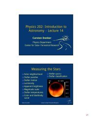
four X-class flares as Flares 1-4, in chronological order <strong>of</strong> <strong>the</strong>ir occurrence. Figure 1 shows <strong>the</strong> history <strong>of</strong><br />
<strong>the</strong> region’s flare production during its 2-week rotation across <strong>the</strong> solar disk. Although <strong>the</strong> region was<br />
highly flare-productive at times, it was by no means a record flare producer, ei<strong>the</strong>r in number <strong>of</strong> flares or<br />
<strong>the</strong>ir s<strong>of</strong>t X-ray class.<br />
Figure 1: Histogram <strong>of</strong> occurrence<br />
<strong>of</strong> flares <strong>of</strong> various s<strong>of</strong>t X-ray<br />
class, B (white), C (green), M (yellow)<br />
<strong>and</strong> X (red), versus date, starting<br />
on <strong>the</strong> day <strong>the</strong> region appeared<br />
on <strong>the</strong> East limb <strong>of</strong> <strong>the</strong> Sun <strong>and</strong><br />
continuing for <strong>the</strong> approximately 2<br />
weeks <strong>of</strong> passage across <strong>the</strong> solar<br />
disk. The region was quite flare<br />
productive <strong>the</strong> first few days, <strong>and</strong><br />
<strong>the</strong>n produced only a small number<br />
<strong>of</strong> C-class flares, with <strong>the</strong> major<br />
exception <strong>of</strong> two X-class flares on<br />
13-14 December. B-class flares<br />
are typically too small to see during<br />
solar maximum, <strong>and</strong> would not<br />
even be reported were it not solar<br />
minimum.<br />
In <strong>the</strong> production <strong>of</strong> radio noise, however, <strong>the</strong> region was a record breaker. The L-b<strong>and</strong> flux density<br />
attained by both <strong>the</strong> 2006 December 6 <strong>and</strong> 13 events (~1 million <strong>and</strong> >300,000 sfu, respectively) exceeded<br />
<strong>the</strong> previous record (165,000 sfu for a burst in April 1973—see Cerruti et al. 2008) by large factors.<br />
The first event on 2006 December 5, in contrast, was not exceptional at L b<strong>and</strong> despite <strong>the</strong> fact that<br />
it was <strong>the</strong> largest <strong>of</strong> <strong>the</strong> four X-class bursts as measured in s<strong>of</strong>t X-rays.<br />
The radio bursts were observed with several radio instruments. We report here on data from <strong>the</strong><br />
four RSTN sites, <strong>the</strong> Owens Valley Solar Array (OVSA) <strong>and</strong> FASR Subsystem Testbed (FST), both in<br />
California, <strong>and</strong> <strong>the</strong> Nobeyama <strong>Radio</strong> Polarimeter (NoRP) in Japan. The RSTN sites each observed one <strong>of</strong><br />
<strong>the</strong> flares, while OVSA <strong>and</strong> FST observed flares 2 <strong>and</strong> 4, <strong>and</strong> NoRP observed flare 3.<br />
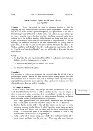
As an example that illustrates some <strong>of</strong> <strong>the</strong> issues, we first show <strong>the</strong> OVSA dynamic spectra for<br />
Flare 2 (Dec 6) in Figure 2. OVSA records data at 39 frequencies between 1.2 <strong>and</strong> 18 GHz, in both senses<br />
<strong>of</strong> circular polarization, with a time resolution <strong>of</strong> 8.1 s (see Nita et al. 2004). It is significant that GPS<br />
transmissions are right circularly polarized (RCP). One <strong>of</strong> <strong>the</strong> clear characteristics <strong>of</strong> <strong>the</strong> December bursts<br />
is that <strong>the</strong>ir L-b<strong>and</strong> emission was also highly RCP. Solar bursts may be highly polarized in ei<strong>the</strong>r sense <strong>of</strong><br />
circular polarization (depending on <strong>the</strong> polarity <strong>of</strong> magnetic field in <strong>the</strong> source region), or may have little<br />
or no polarization. Only <strong>the</strong> RCP component <strong>of</strong> <strong>the</strong> solar emission can affect GPS receivers. Figure 2a<br />
shows radio flux density in a logarithmic scale, with black representing low radio flux density <strong>and</strong> white<br />
representing high flux density. The scale ranges from 1 to 10 4 sfu, so emission greater than 10 4 sfu is saturated.<br />
Note especially <strong>the</strong> strong, saturated emission below 2 GHz in <strong>the</strong> RCP, while in LCP it is unsaturated.<br />
The radio burst lasted about 1 h 40 m <strong>and</strong>, except for <strong>the</strong> strong L-b<strong>and</strong> RCP emission, <strong>the</strong> burst is<br />
quite typical <strong>of</strong> large flares. OVSA maintains a high dynamic range by inserting attenuation in <strong>the</strong> re-<br />
2
ceiver to keep <strong>the</strong> signal in range, based on <strong>the</strong> measured flux density in <strong>the</strong> previously measured sample<br />
8.1 s earlier. However, when <strong>the</strong> fluctuations in flux density are too rapid, <strong>the</strong> system may have too little<br />
attenuation <strong>and</strong> will <strong>the</strong>n saturate. Such points are flagged as bad data, <strong>and</strong> appear black in Fig. 2. This is<br />
especially noticeable at <strong>the</strong> lowest frequency, 1.2 GHz.<br />
Figure 2: OVSA dynamic spectrum <strong>of</strong> <strong>the</strong> largest <strong>of</strong> <strong>the</strong> radio bursts, <strong>the</strong> 2006 Dec 06 event. a) right circular<br />
polarization (RCP). b) left circular polarization (LCP). The flux density scale ranges logarithmically from 1<br />
to 10 4 sfu, so <strong>the</strong> very bright RCP L-b<strong>and</strong> emission (1-2 GHz) is saturated on this scale <strong>and</strong> appears white.<br />
True saturation (see text) causes <strong>the</strong> data to be flagged as bad data, <strong>and</strong> appears black in <strong>the</strong> figure, which is<br />
especially noticeable at 1.2 GHz. The brightest L-b<strong>and</strong> RCP emission occurs between 19:30 <strong>and</strong> 19:40 UT,<br />
<strong>and</strong> causes instrumental artifacts at higher frequencies (between 15-18 GHz, <strong>and</strong> at times at o<strong>the</strong>r frequencies<br />
as well).<br />
Fortunately, at <strong>the</strong> time <strong>of</strong> <strong>the</strong>se flares a new instrument was operating at Owens Valley, <strong>the</strong> FASR<br />
Subsystem Testbed (Liu et al. 2007), which was observing at extremely high time <strong>and</strong> frequency resolution<br />
(20 ms <strong>and</strong> 977 kHz, respectively) in <strong>the</strong> b<strong>and</strong> 1.0-1.5 GHz, so we can in effect zoom in on this portion<br />
<strong>of</strong> <strong>the</strong> spectrum as shown in Figure 3. The time resolution in Fig. 3 has been vastly reduced to match<br />
<strong>the</strong> OVSA time resolution, for display purposes, but we will use <strong>the</strong> full resolution in §4 where we discuss<br />
<strong>the</strong> physical origin <strong>of</strong> <strong>the</strong> emission. Although <strong>the</strong> emission in Fig. 3 appears relatively smooth <strong>and</strong> featureless,<br />
it in fact exhibits extreme variability at shorter time scales.<br />
Figure 3: FST dynamic spectrum <strong>of</strong> <strong>the</strong> 1.0-1.5 GHz RCP emission, scaled logarithmically from 1 to 10 6 sfu.<br />
The time resolution <strong>of</strong> <strong>the</strong> FST instrument has been vastly reduced, to 8 s to match <strong>the</strong> OVSA data, but it is<br />
actually far better, at 20 ms, allowing us to unambiguously determine <strong>the</strong> emission mechanism.<br />
3
The main points to draw from Figs. 2 <strong>and</strong> 3 are that <strong>the</strong> burst emits over a broad range <strong>of</strong> frequencies,<br />
<strong>and</strong> that in <strong>the</strong> L-b<strong>and</strong> it produced vast amounts <strong>of</strong> radio noise in RCP. GPS operates at two frequencies,<br />
<strong>the</strong> so-called L1 frequency at 1575 MHz, <strong>and</strong> L2 at 1227 MHz (see Cerruti et al. 2008 for more details),<br />
so this L-b<strong>and</strong> emission is highly significant for GPS receivers.<br />
The RSTN stations operate at 8 frequencies, 245, 410, 610, 1415, 2695, 4995, 8400, <strong>and</strong> 15400<br />
MHz, <strong>and</strong> records data only in total intensity (no polarization information). The 1415 MHz frequency is<br />
<strong>the</strong> one <strong>of</strong> interest for potential impact on GPS <strong>and</strong> o<strong>the</strong>r navigation systems. Peak flux densities were<br />
reported for all four X-class events, from four different RSTN stations. As shown in Table 1, <strong>the</strong> RSTN<br />
flux was reported to be less than <strong>the</strong> peak L-b<strong>and</strong> flux for three <strong>of</strong> <strong>the</strong> four events, but for different reasons<br />
that will be discussed in §3.<br />
Flare<br />
Number<br />
Table 1: Reported L-B<strong>and</strong> <strong>Flux</strong> vs. Actual Peak <strong>Flux</strong> for X-Class Events<br />
Date <strong>of</strong> X-Flare S<strong>of</strong>t X-ray<br />
Class<br />
RSTN<br />
Station<br />
RSTN 1400 MHz<br />
<strong>Flux</strong> Reported<br />
Actual L-b<strong>and</strong><br />
Peak <strong>Flux</strong><br />
1 2006 Dec 05 X9.0 San Vito 3,900 3,900<br />
2 2006 Dec 06 X6.5 Sagamore Hill 13,000 ~1,000,000<br />
3 2006 Dec 13 X3.4 Learmonth 130,000 440,000 (1 GHz)<br />
4 2006 Dec 14 X1.5 Palehua 2,700 120,000<br />
The NoRP instrument operates at 7 frequencies, 1000, 2000, 3750, 9400, 17000, 35000 <strong>and</strong> 80000<br />
MHz, <strong>and</strong> records both RCP <strong>and</strong> LCP flux densities. Only Flare 3 occurred during <strong>the</strong> NoRP observing<br />
time, <strong>and</strong> its L-b<strong>and</strong> frequencies bracket <strong>the</strong> 1415 MHz RSTN frequency, so comparisons are inexact, but<br />
<strong>the</strong> reported flux densities <strong>of</strong> 440,000 sfu at 1 GHz <strong>and</strong> 302,000 sfu at 2 GHz suggest that <strong>the</strong> 1415 MHz<br />
flux density falls somewhere in <strong>the</strong> range 3-4×10 5 sfu.<br />
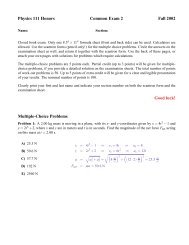
RSTN radio flux density time pr<strong>of</strong>iles at 1415 <strong>and</strong> 2695 MHz are shown in Figure 4 for Flares 1<br />
<strong>and</strong> 3, in order to contrast <strong>the</strong>ir radio behavior. Although <strong>the</strong> s<strong>of</strong>t X-ray class <strong>of</strong> <strong>the</strong> X9.0 event on December<br />
5 exceeds that <strong>of</strong> <strong>the</strong> X3.4 event on December 13, <strong>the</strong> order <strong>of</strong> <strong>the</strong>ir relative radio output is reversed.<br />
The smaller s<strong>of</strong>t X-ray event (Flare 3) was a much greater producer <strong>of</strong> radio emission. We discuss<br />
this fur<strong>the</strong>r in §4.<br />
4<br />
Figure 4: <strong>Radio</strong> flux density at two frequencies<br />
for Flares 1 <strong>and</strong> 3, recorded at<br />
RSTN sites. a) Flare 1, recorded on 2006<br />
December 05 at San Vito, Italy, displays<br />
typical flux density levels for a large<br />
flare, reaching about 10,000 sfu at 2695<br />
MHz, <strong>and</strong> showing a relatively smooth<br />
time pr<strong>of</strong>ile. b) The same flare at 1415<br />
MHz reached only 3900 sfu. c) Flare 3,<br />
recorded on 2006 December 13 at Learmonth,<br />
Australia, at 2695 GHz, displays<br />
rapid variations <strong>and</strong> stays at elevated flux<br />
levels for several hours. d) The same flare<br />
at 1415 MHz, showing that <strong>the</strong> flux density<br />
increases at lower frequencies, typical<br />
<strong>of</strong> <strong>the</strong> bursts affecting GPS systems. Note<br />
that <strong>the</strong> highest peaks at 1415 MHz are<br />
clipped at <strong>the</strong> 100,000 sfu saturation level<br />
<strong>of</strong> <strong>the</strong> RSTN receivers.
3. Effects <strong>of</strong> Saturation on Measurements <strong>of</strong> <strong>Radio</strong> Noise Level<br />
In order to assess <strong>the</strong> threat <strong>of</strong> solar radio bursts to wireless systems, we need a way to determine<br />
<strong>the</strong> likelihood <strong>of</strong> occurrence <strong>of</strong> bursts exceeding some threshold for harmful effects. An obvious way to<br />
do this is to consult <strong>the</strong> historical record, which was <strong>the</strong> approach taken by Nita et al. (2002, 2004). However,<br />
Figure 5, adapted from Nita et al. (2002), shows that <strong>the</strong> largest bursts in <strong>the</strong> 1-2 GHz frequency<br />
range appear to be missing from <strong>the</strong> data. There is a clear cut<strong>of</strong>f at about 10 5 sfu in <strong>the</strong> distribution <strong>of</strong><br />
bursts occurring at solar maximum. The occurrence <strong>of</strong> <strong>the</strong> 2006 December events shows that large bursts<br />
do occur, <strong>and</strong> that <strong>the</strong> cut<strong>of</strong>f may be due to instrumental saturation. Even <strong>the</strong> extrapolated distribution,<br />
however, would predict <strong>the</strong> 2006 December 6 event to occur only once in 100 years at solar minimum. We<br />
briefly examine <strong>the</strong> way <strong>the</strong>se bursts affected <strong>the</strong> RSTN <strong>and</strong> OVSA radio instruments, <strong>and</strong> by implication,<br />
how saturation may have affected <strong>the</strong> historical record.<br />
Figure 5: Distribution <strong>of</strong> sizes (peak<br />
flux densities) <strong>of</strong> solar radio bursts<br />
over 40 years <strong>of</strong> burst reports from<br />
NOAA, separated into bursts occurring<br />
within 2 years <strong>of</strong> solar maximum <strong>and</strong><br />
those occurring within 2 years <strong>of</strong> solar<br />
minimum (see Nita et al. 2002 for details).<br />
The horizontal scale gives <strong>the</strong><br />
number <strong>of</strong> days between bursts. Both<br />
distributions show an apparent cut<strong>of</strong>f<br />
in flux density, i.e. <strong>the</strong> highest flux<br />
density bursts are missing. Note that<br />
extrapolating <strong>the</strong> distributions to 10 6<br />
sfu predicts such bursts should occur<br />
once every 10 solar maximum years<br />
(about once every 25 years), or once in<br />
41 solar minimum years (about 100<br />
years).<br />
Different receiver designs will be affected by saturation in different ways. The RSTN data from<br />
Learmonth for Flare 3 (Fig. 4d) shows one way that receivers may react, by simply clipping <strong>the</strong> signal at<br />
<strong>the</strong>ir design limit. However, <strong>the</strong> fluxes reported by RSTN sites for Flares 2 <strong>and</strong> 4 (Table 1) are far below<br />
those measured by OVSA, suggesting a different failure mode for those sites. Unfortunately, <strong>the</strong> detailed<br />
records for <strong>the</strong>se two flares are not yet available at NOAA, so we have only <strong>the</strong> peak flux reports.<br />
OVSA, too, suffered saturation <strong>of</strong> at least two different kinds during <strong>the</strong> largest burst (Flare 2) on<br />
2006 December 6. One type <strong>of</strong> saturation results in data being unrecoverably lost due to incorrect attenuation<br />
inserted into <strong>the</strong> system. This results in overdriving <strong>the</strong> A/D converter, <strong>and</strong> causes <strong>the</strong> unrecoverable<br />
loss <strong>of</strong> data shown in Fig. 2, especially at 1.2 GHz. The o<strong>the</strong>r type <strong>of</strong> saturation is more subtle, where<br />
<strong>the</strong>re is an in-range measurement, but due to non-linear amplifier response <strong>the</strong> measured flux density is<br />
lower than its true flux density. The OVSA measurements are made in parallel on several nominally identical<br />
antennas, <strong>and</strong> by plotting <strong>the</strong> flux density measured on one antenna versus ano<strong>the</strong>r we do see such<br />
nonlinearity. However, lacking a clear preference for one antenna over ano<strong>the</strong>r, we use <strong>the</strong> average value<br />
<strong>of</strong> <strong>the</strong>se independent measurements. Thus, although it could be argued that <strong>the</strong> antenna measuring <strong>the</strong><br />
highest flux density suffered <strong>the</strong> least saturation, we take <strong>the</strong> more conservative average keeping in mind<br />
that <strong>the</strong> true flux density could be higher.<br />
We now wish to transfer OVSA’s absolute flux density scale to <strong>the</strong> FST data, which are available<br />
at much higher time <strong>and</strong> frequency resolution. To do this, we have to identify <strong>the</strong> specific times in <strong>the</strong><br />
FST data <strong>and</strong> integrate over <strong>the</strong> same b<strong>and</strong>width as covered by <strong>the</strong> OVSA receivers. Figure 6 shows a<br />
30 s segment <strong>of</strong> <strong>the</strong> FST data at full resolution, with small boxes outlining <strong>the</strong> durations <strong>and</strong> b<strong>and</strong>widths <strong>of</strong><br />
individual OVSA measurements at 1.2 <strong>and</strong> 1.4 GHz. Integrating over <strong>the</strong>se boxes, we obtain <strong>the</strong> exact<br />
data for comparison with OVSA <strong>and</strong> transfer <strong>of</strong> <strong>the</strong> calibration. Figure 7 shows <strong>the</strong> FST measurements<br />
integrated over <strong>the</strong> regions like <strong>the</strong> examples in Fig. 6, overplotted with appropriate scaling to match <strong>the</strong><br />
OVSA data.<br />
Fig. 7 shows that <strong>the</strong> two instruments agree to a high degree <strong>of</strong> precision except for <strong>the</strong> period<br />
around 18:50 UT, when <strong>the</strong> FST gain control malfunctioned for a time. FST uses signals from three <strong>of</strong> <strong>the</strong><br />
5
Figure 6: A 30 s <strong>of</strong> period <strong>of</strong> FST data at full resolution, for Flare 2, showing <strong>the</strong> times <strong>and</strong> b<strong>and</strong>widths <strong>of</strong> <strong>the</strong><br />
OVSA measurements at 1.2 <strong>and</strong> 1.4 GHz. OVSA is a double-sideb<strong>and</strong> system, so it covers sideb<strong>and</strong>s on ei<strong>the</strong>r<br />
side <strong>of</strong> <strong>the</strong> nominal frequency. The alternating brighter <strong>and</strong> darker b<strong>and</strong>s <strong>of</strong> 4 s duration (8.1 s period)<br />
are due to switching circular polarization. The brighter b<strong>and</strong>s are RCP, <strong>and</strong> show thous<strong>and</strong>s <strong>of</strong> densely<br />
packed spike bursts. The darker b<strong>and</strong>s are LCP, <strong>and</strong> are dominated by instrumental artifacts caused by crosstalk<br />
from <strong>the</strong> RCP feed, hence should be ignored. The integrated flux density in such boxes for <strong>the</strong> entire duration<br />
<strong>of</strong> <strong>the</strong> burst is shown in Fig. 7.<br />
Figure 7: <strong>Radio</strong> flux density<br />
at two frequencies for<br />
<strong>the</strong> event <strong>of</strong> 2006 December<br />
6, comparing <strong>the</strong><br />
OVSA measurements (+<br />
symbols) with <strong>the</strong> FST<br />
measurements integrated<br />
over <strong>the</strong> identical times<br />
<strong>and</strong> b<strong>and</strong>widths as in Fig.<br />
6. The FST data <strong>of</strong> uncalibrated<br />
flux density are<br />
scaled with a fixed multiplicative<br />
factor to match<br />
<strong>the</strong> OVSA points, which<br />
yields <strong>the</strong> factor needed to<br />
transfer OVSA’s calibration<br />
to FST.<br />
OVSA dishes, but two <strong>of</strong> <strong>the</strong> FST receivers suffered saturation during <strong>the</strong> highest peaks, especially during<br />
<strong>the</strong> period that most affected <strong>the</strong> GPS receivers, from 19:30-19:40 UT. This causes a visible suppression<br />
(not shown) <strong>of</strong> <strong>the</strong> peaks in <strong>the</strong> data from those two antennas relative to <strong>the</strong> third. The overall peak flux<br />
densities for <strong>the</strong> 2006 December 6 event, as measured with OVSA are 6.5×10 5 sfu at 1.2 GHz, 1×10 6 sfu<br />
at 1.4 GHz, <strong>and</strong> 5×10 5 sfu at 1.6 GHz. However, recall that sfu is a flux density, with units W m -2 Hz -1 ,<br />
<strong>and</strong> so <strong>the</strong>se values represent an average flux over <strong>the</strong> OVSA b<strong>and</strong>width (roughly 100 MHz). The relevant<br />
GPS b<strong>and</strong>width is much smaller (1 or 10 MHz, depending on <strong>the</strong> GPS receiver operation), <strong>and</strong> as Fig.<br />
6 shows <strong>the</strong> radio emission occurs in very narrow b<strong>and</strong>, short-duration spikes.<br />
Using FST data, we plot flux densities integrated over 10 MHz in Figure 8 during <strong>the</strong> highest-flux<br />
period, 19:30-19:40 UT. We find that <strong>the</strong> flux density momentarily reaches peak levels <strong>of</strong> 1.85×10 6 sfu at<br />
1.227 MHz (<strong>the</strong> GPS L2 frequency) <strong>and</strong> 2.5×10 6 sfu at 1.405 MHz (for comparison with RSTN). Note<br />
that <strong>the</strong> fluctuations in Fig. 8 are not statistical noise. As discussed by Nita et al. (2007), <strong>the</strong> statistical<br />
signal to noise ratio for a single power measurement is exactly 1 for Gaussian noise, so after averaging<br />
over M time samples <strong>and</strong> N frequencies, <strong>the</strong> signal to noise ratio will be 1 / MN . Each point in Fig. 8<br />
represents an average over M = 122 time samples <strong>and</strong> N = 10 frequencies, for a signal to noise ratio <strong>of</strong><br />
about 0.03. This is about 20 times smaller than <strong>the</strong> fluctuations in Fig. 8. The extreme variability <strong>of</strong> <strong>the</strong><br />
solar signal on such short time <strong>and</strong> narrow frequency scales means that gauging <strong>the</strong> effect <strong>of</strong> solar radio<br />
noise on GPS receivers requires solar observations using high resolution spectrographic data like that provided<br />
by FST <strong>and</strong> o<strong>the</strong>r spectrographs around <strong>the</strong> world.<br />
6
Figure 8: Full resolution<br />
RCP flux density, integrated<br />
over 10 MHz b<strong>and</strong>width a)<br />
for GPS L2 frequency, b) for<br />
1.4 GHz. The gaps are periods<br />
when LCP was being<br />
measured The variations in<br />
each 4 s <strong>of</strong> data points is due<br />
to true variations in <strong>the</strong> solar<br />
signal, <strong>and</strong> are not statistical<br />
noise. Therefore, <strong>the</strong> points<br />
above <strong>the</strong> 10 6 sfu level (indicated<br />
by <strong>the</strong> horizontal line in<br />
each plot) are significant.<br />
4. Emission Mechanism <strong>and</strong> Physical Conditions Responsible for <strong>the</strong> Solar <strong>Flux</strong> <strong>Density</strong><br />
From <strong>the</strong> spectral signature <strong>of</strong> <strong>the</strong> emission seen in Fig. 6, especially near <strong>the</strong> end <strong>of</strong> <strong>the</strong> 30 s period<br />
shown, we see that <strong>the</strong> emission is made up <strong>of</strong> extremely narrow-b<strong>and</strong> (3-5 MHz) spikes <strong>of</strong> short duration<br />
(< 20 ms). Such bursts are well known, <strong>and</strong> are not surprisingly called spike bursts (Slottje 1978).<br />
However, in those bursts where such spikes are seen, generally <strong>the</strong> number <strong>of</strong> spikes is in <strong>the</strong> hundreds to<br />
thous<strong>and</strong>s (e.g. Csillaghy & Benz 1993), <strong>and</strong> although <strong>the</strong>y can occur in clusters, <strong>the</strong>y usually last for only<br />
a few minutes <strong>and</strong> are sufficiently separated that individual spikes can be seen. During more than 40 minutes<br />
<strong>of</strong> <strong>the</strong> 2006 December 6 event, <strong>the</strong> spikes were so numerous as to blend into a single highly fluctuating<br />
level <strong>of</strong> emission, only becoming individually distinguishable near <strong>the</strong> end <strong>of</strong> <strong>the</strong> burst, as shown in<br />
Fig. 6. A simple estimate <strong>of</strong> number <strong>of</strong> spikes (assuming no overlap) to fill a 500 MHz b<strong>and</strong>width for 40<br />
minutes requires more than 10 million spikes to have been produced during this burst.<br />
As mentioned in §1, <strong>the</strong> ECM mechanism is thought to be responsible spike bursts (see Treumann<br />
2006 for a general review, <strong>and</strong> Fleishman 2006 for a review <strong>of</strong> <strong>the</strong> solar burst case). This coherent<br />
mechanism is naturally highly polarized, <strong>and</strong> is due to high-energy electrons mirroring in <strong>the</strong> converging<br />
field <strong>of</strong> a closed magnetic loop, where <strong>the</strong>y form a loss-cone distribution that is unstable to catastrophic<br />
wave growth (Wu & Lee 1979; Holman et al. 1980; Melrose & Dulk 1982). The emission occurs near <strong>the</strong><br />
cyclotron frequency or its low harmonics, which requires a magnetic field strength <strong>of</strong> order 450 G. To<br />
maintain <strong>the</strong> instability requires replenishment <strong>of</strong> <strong>the</strong> high-energy electrons, which implies sustained acceleration<br />
<strong>and</strong> excellent trapping over 40 minutes (see Rozhansky et al. 2008, where <strong>the</strong> local source<br />
model is discussed in some detail). Such trapping in turn requires relatively low density in <strong>the</strong> loop<br />
(Fleishman et al. 2003) to avoid collisional energy loss. One can estimate <strong>the</strong> density assuming that collisional<br />
energy loss <strong>of</strong> electrons <strong>of</strong> energy ~100 keV (e.g. eq. 4 <strong>of</strong> Bastian et al. 2007) causes <strong>the</strong> long exponential<br />
decay (time constant about 208 s) visible in Fig. 7 after <strong>the</strong> spikes turn <strong>of</strong>f around 1940 UT. The<br />
implied density is around 10 9 cm -3 , <strong>and</strong> even lower for lower energy electrons; hence such loops are generally<br />
not visible in EUV or X-ray images. The instability in a given volume <strong>of</strong> plasma is quickly<br />
quenched (within < 20 ms, which accounts for <strong>the</strong> short duration <strong>of</strong> <strong>the</strong> spikes), so to create 10 million<br />
spikes requires that <strong>the</strong>se appropriate conditions be satisfied again <strong>and</strong> again, at many places in <strong>the</strong> loop<br />
simultaneously. One might consider such conditions to occur only very rarely, except that we know that<br />
<strong>the</strong>y occurred three times within one week in AR 10930. This strongly suggests that AR 10930 maintained<br />
a magnetic configuration highly favorable for <strong>the</strong> production <strong>of</strong> ECM emission. Because <strong>the</strong> historical<br />
record appears to be incomplete, it remains uncertain how <strong>of</strong>ten such conditions occur.<br />
5. Conclusion<br />
We have given an overview <strong>of</strong> <strong>the</strong> flares in AR 10390 during 2006 December, have placed <strong>the</strong>se<br />
bursts in <strong>the</strong> context <strong>of</strong> <strong>the</strong> historical record, <strong>and</strong> have attempted to obtain a reliable L-b<strong>and</strong> flux density<br />
for <strong>the</strong> largest <strong>of</strong> <strong>the</strong> events, <strong>the</strong> event <strong>of</strong> 2006 December 6. We have also briefly examined <strong>the</strong> solar conditions<br />
causing <strong>the</strong> extreme solar radio flux densities observed. Our main conclusions are as follows:<br />
• The cause <strong>of</strong> <strong>the</strong> extreme flux density is an unusually high density <strong>of</strong> spike bursts due to <strong>the</strong><br />
Electron-Cyclotron Maser mechanism.<br />
7
• The December 6 event reached a flux density <strong>of</strong> at least 10 6 sfu at 1.4 GHz, momentarily<br />
reaching flux densities as high as 2.5×10 6 sfu during individual spikes.<br />
• Bursts <strong>of</strong> 10 6 sfu, if <strong>the</strong>y follow <strong>the</strong> general size distribution <strong>of</strong> solar bursts, should occur once<br />
every 25 years at solar maximum rates, or once every 100 years at solar minimum rates. The<br />
events <strong>of</strong> 2006 December 6 are <strong>the</strong>refore extremely rare occurrences.<br />
• In <strong>the</strong> historical record, however, <strong>the</strong> largest bursts are missing, <strong>and</strong> we argue that it may be<br />
due to instrumental saturation. This leaves open <strong>the</strong> question <strong>of</strong> how <strong>of</strong>ten such large events<br />
may occur.<br />
• To monitor <strong>the</strong> effects <strong>of</strong> solar bursts on GPS, GLONASS, <strong>and</strong> Galileo navigation systems, a<br />
world-wide network <strong>of</strong> solar spectrographs is needed that can measure right-circularly polarized<br />
emission at L-b<strong>and</strong> with high frequency <strong>and</strong> time resolution, without saturation.<br />
As our society becomes ever more dependent on wireless technology, <strong>the</strong> effects <strong>of</strong> solar radio bursts can<br />
be expected to appear more <strong>of</strong>ten. Mission-critical systems should be designed with solar radio emission<br />
in mind. A warning system based on an improved set <strong>of</strong> world-wide instrumentation could be implemented<br />
at relatively low cost, taking advantage <strong>of</strong> new technology that allows broadb<strong>and</strong> digital signal<br />
measurements. Ultimately, such extreme flux density bursts need to be studied at high spatial resolution<br />
with arrays such as <strong>the</strong> proposed Frequency Agile Solar <strong>Radio</strong>telescope (FASR) in order to better underst<strong>and</strong><br />
<strong>the</strong> conditions leading to <strong>the</strong>ir occurrence, <strong>and</strong> ultimately to be able to predict such events.<br />
6. Acknowledgments<br />
This work was supported by NSF grants ATM-0707319, AST-0352915 <strong>and</strong> AST-0607544, <strong>and</strong><br />
NASA grant NNG06GJ40G to New Jersey Institute <strong>of</strong> Technology.<br />
References<br />
Afraimovich, E.L., Zherebtsov G.A., <strong>and</strong> Smolkov G.Ya. 2007, Total Failure <strong>of</strong> GPS during a solar flare on December<br />
6, 2006. Doklady Earth Sciences 417 (8), 1231<br />
Afraimovich, E. L., Demyanov, V. V., Gary, D. E., Ishin, A. B. <strong>and</strong> Smolkov, G. Ya. 2008, Failure <strong>of</strong> GPS functioning<br />
caused by extreme solar radio events, IES 2008 (this proceedings).<br />
Bastian, T.S., Fleishman, G.D. & Gary, D.E. 2007, <strong>Radio</strong> Spectral Evolution <strong>of</strong> an X-Ray-poor Impulsive Solar<br />
Flare: Implications for Plasma Heating <strong>and</strong> Electron Acceleration, ApJ, 666, 1256<br />
Cerruti, A.P., Kintner, P.M., Gary, D.E., Lanzerotti, L.J., E.R. de Paula, Vo, H.B., 2006. Observed Solar <strong>Radio</strong> Burst<br />
Effects on GPS/WAAS Carrier-to-Noise Ration. Space Wea<strong>the</strong>r 4, S10006<br />
Cerruti, A.P., Kintner, P.M., Gary, D.E., Mannucci, A.J., Meyer, R.F., Doherty, P. & Coster, A.J. 2008, The effect <strong>of</strong><br />
intense December 2006 solar radio bursts on GPS receivers, Space Wea<strong>the</strong>r, in press.<br />
Chen, Z., Gao Y., <strong>and</strong> Liu Z., 2005. Evaluation <strong>of</strong> solar radio bursts' effect on GPS receiver signal tracking within<br />
International GPS Service network. <strong>Radio</strong> Science 40, RS3012, doi:10.1029/2004RS003066.<br />
Csillaghy, A. & Benz, A. O. 1993, The b<strong>and</strong>width <strong>of</strong> millisecond radio spikes in solar flares, A&A, 274, 487<br />
Fleishman, G.D. 2006, in Solar Physics with <strong>the</strong> Nobeyama <strong>Radio</strong>heliograph, ed. K. Shibasaki et al. (NSRO Rep. 1)<br />
(Nobeyama: Nobeyama Sol. <strong>Radio</strong> Obs.), 51<br />
Fleishman, G., Gary, D.E. & Nita, G.M. 2003, Decimetric spike bursts versus microwave continuum, ApJ, 592, 571<br />
Holman, G.D., Eichler, D. & Kundu, M.R. 1980, An interpretation <strong>of</strong> solar flare microwave spikes as gyrosynchrotron<br />
mastering, in <strong>Radio</strong> physics <strong>of</strong> <strong>the</strong> Sun, IAU Symposium 86, 457<br />
Liu, Z., Gary, D.E., Nita, G.M., White, S.M. & Hurford, G.J. 2007, PASP, A subsystem test bed for <strong>the</strong> Frequency-<br />
Agile Solar <strong>Radio</strong>telescope, 119, 303<br />
Melrose, D.B. & Dulk, G.A. 1982, Electron-cyclotron masers as <strong>the</strong> source <strong>of</strong> certain solar <strong>and</strong> stellar radio bursts,<br />
ApJ, 259, 844<br />
Nita, G.M., Gary, D., Lanzerotti, L. & Thomson, D. 2002. Peak flux distribution <strong>of</strong> solar radio bursts, ApJ, 570, 423.<br />
Nita, G.M., Gary, D.E. & Lee, J. 2004, Statistical study <strong>of</strong> two years <strong>of</strong> solar flare radio spectra obtained with <strong>the</strong><br />
Owens Valley Solar Array, ApJ, 605, 528<br />
Nita, G.M., Gary, D.E., Liu, Z., Hurford, G. & White, S.M. 2007, <strong>Radio</strong> frequency interference excision using spectral-domain<br />
statistics, PASP, 119, 805<br />
Kintner, P.M. 2008, An overview <strong>of</strong> solar radio bursts <strong>and</strong> GPS, IES 2008, this proceedings.<br />
Klobuchar, J. A., Kunches, J. M., Van Dierendonck, A. J., 1999. Eye on <strong>the</strong> ionosphere: Potential solar radio<br />
burst effects on GPS signal to noise. GPS Solutions 3(2), 69<br />
Rozhansky, I.V.; Fleishman, G.D.; Huang, G.-L. 2008, Millisecond microwave spikes: statistical study<br />
<strong>and</strong> application for plasma diagnostics, Astro-ph/0803.2380 (ApJ, accepted)<br />
Slottje, C. 1978, Millisecond microwave spikes in a solar flare, Nature 275, 520<br />
Treuman, R. 2006, The electron cyclotron maser for astrophysical application, A&ARv, 13, 229<br />
Wu, C.S. & Lee, L.C. 1979, A <strong>the</strong>ory <strong>of</strong> <strong>the</strong> terrestrial kilometric radiation, ApJ, 230, 621<br />
8