Underwater SLAM in man-made structured environments - robotics ...
Underwater SLAM in man-made structured environments - robotics ...
Underwater SLAM in man-made structured environments - robotics ...

You also want an ePaper? Increase the reach of your titles
YUMPU automatically turns print PDFs into web optimized ePapers that Google loves.
<strong>Underwater</strong> <strong>SLAM</strong> <strong>in</strong><br />
Man-Made Structured<br />
Environments<br />
• • • • • • • • • • • • • • • • • • • • • • • • • • • • • • •<br />
1. INTRODUCTION<br />
David Ribas and Pere Ridao<br />
Grup de Visió per Computador i Robòtica<br />
Universitat de Girona<br />
Girona 17071, Spa<strong>in</strong><br />
e-mail: dribas@eia.udg.es, pere@eia.udg.es<br />
Juan Dom<strong>in</strong>go Tardós and José Neira<br />
Grupo de Robótica y Tiempo Real<br />
Universidad de Zaragoza<br />
Zaragoza 50018, Spa<strong>in</strong><br />
e-mail: tardos@unizar.es, jneira@unizar.es<br />
Received 9 January 2008; accepted 30 May 2008<br />
This paper describes a navigation system for autonomous underwater vehicles (AUVs)<br />
<strong>in</strong> partially <strong>structured</strong> <strong>environments</strong>, such as dams, harbors, mar<strong>in</strong>as, and mar<strong>in</strong>e platforms.<br />
A mechanically scanned imag<strong>in</strong>g sonar is used to obta<strong>in</strong> <strong>in</strong>formation about the<br />
location of vertical planar structures present <strong>in</strong> such <strong>environments</strong>. A robust vot<strong>in</strong>g algorithm<br />
has been developed to extract l<strong>in</strong>e features, together with their uncerta<strong>in</strong>ty, from the<br />
cont<strong>in</strong>uous sonar data flow. The obta<strong>in</strong>ed <strong>in</strong>formation is <strong>in</strong>corporated <strong>in</strong>to a feature-based<br />
simultaneous localization and mapp<strong>in</strong>g (<strong>SLAM</strong>) algorithm runn<strong>in</strong>g an extended Kal<strong>man</strong><br />
filter. Simultaneously, the AUV’s position estimate is provided to the feature extraction algorithm<br />
to correct the distortions that the vehicle motion produces <strong>in</strong> the acoustic images.<br />
Moreover, a procedure to build and ma<strong>in</strong>ta<strong>in</strong> a sequence of local maps and to posteriorly<br />
recover the full global map has been adapted for the application presented. Experiments<br />
carried out <strong>in</strong> a mar<strong>in</strong>a located <strong>in</strong> the Costa Brava (Spa<strong>in</strong>) with the Ict<strong>in</strong>eu AUV show the<br />
viability of the proposed approach. C○ 2008 Wiley Periodicals, Inc.<br />
Simultaneous localization and mapp<strong>in</strong>g (<strong>SLAM</strong>) is<br />
one of the fundamental problems that needs to be<br />
solved before achiev<strong>in</strong>g truly autonomous vehicles.<br />
For this reason, <strong>in</strong> recent years it has been the focus<br />
of a great deal of attention (see Bailey & Durrant-<br />
Whyte, 2006; Durrant-Whyte & Bailey, 2006, and references<br />
there<strong>in</strong>). Multiple techniques have shown<br />
promis<strong>in</strong>g results <strong>in</strong> a variety of different applications<br />
and scenarios. Some of them perform <strong>SLAM</strong> <strong>in</strong>doors<br />
Journal of Field Robotics, 1–24 (2008) C○ 2008 Wiley Periodicals, Inc.<br />
Published onl<strong>in</strong>e <strong>in</strong> Wiley InterScience (www.<strong>in</strong>terscience.wiley.com). • DOI: 10.1002/rob.20249<br />
(Castellanos, Montiel, Neira, & Tardós, 1999), outdoors<br />
(Guivant, Nebot, & Durrant-Whyte, 2000), and<br />
even on air (Kim & Sukkarieh, 2003). However, the<br />
underwater environment is still one of the most challeng<strong>in</strong>g<br />
scenarios for <strong>SLAM</strong> because of the reduced<br />
sensorial possibilities and the difficulty <strong>in</strong> f<strong>in</strong>d<strong>in</strong>g reliable<br />
features. Acoustic devices are the most common<br />
choice. Many approaches extract features from<br />
acoustic data produced by imag<strong>in</strong>g sonars (Leonard,<br />
Carpenter, & Feder, 2001; Tena, Petillot, Lane, &<br />
Salson, 2001) or sidescan sonars (Tena, Reed, Petillot,
2 • Journal of Field Robotics—2008<br />
Bell, & Lane, 2003). Some <strong>in</strong>troduce artificial beacons<br />
to deal with complex <strong>environments</strong> (New<strong>man</strong><br />
& Leonard, 2003; Williams, New<strong>man</strong>, Rosenblatt,<br />
Dissanayake, & Durrant-Whyte, 2001). An alternative<br />
approach is analyz<strong>in</strong>g the three-dimensional (3D)<br />
structure of the environment to perform <strong>SLAM</strong>, either<br />
us<strong>in</strong>g bathymetric scans (Ro<strong>man</strong> & S<strong>in</strong>gh, 2005)<br />
or produc<strong>in</strong>g a tessellated representation of the scenario<br />
(Fairfield, Jonak, Kantor, & Wettergreen, 2007).<br />
The use of cameras is limited to applications <strong>in</strong> which<br />
the vehicle navigates <strong>in</strong> clear water and very near<br />
to the seafloor (Eustice, S<strong>in</strong>gh, Leonard, Walter, &<br />
Ballard, 2005). On the other hand, the visual <strong>in</strong>formation<br />
can also be comb<strong>in</strong>ed with acoustic data to<br />
improve the overall reliability of the <strong>SLAM</strong> system<br />
(Williams & Mahon, 2004).<br />
This article focuses on underwater <strong>SLAM</strong> applied<br />
to <strong>man</strong>-<strong>made</strong> <strong>environments</strong> (harbors, mar<strong>in</strong>as,<br />
mar<strong>in</strong>e platforms, dams, etc.) where structures composed<br />
of vertical planes are present and produce<br />
reliable features <strong>in</strong> acoustic images. Although most<br />
of the previous work done <strong>in</strong> this field focuses on<br />
open sea and coastal applications, obta<strong>in</strong><strong>in</strong>g an accurate<br />
position<strong>in</strong>g <strong>in</strong> such scenarios would notably<br />
<strong>in</strong>crease autonomous underwater vehicle (AUV) capabilities.<br />
For <strong>in</strong>stance, an AUV could use a harbor<br />
as an outpost for oceanography research if it is<br />
able to localize itself and navigate through it with<br />
enough accuracy to safely perform the leav<strong>in</strong>g and<br />
return<strong>in</strong>g operations (Griffiths, McPhail, Rogers, &<br />
Meldrum, 1998). Ma<strong>in</strong>tenance and <strong>in</strong>spection of underwater<br />
structures (Mart<strong>in</strong>s, Matos, Cruz, & Pereira,<br />
1999) and even surveillance of mar<strong>in</strong>e <strong>in</strong>stallations<br />
are examples of other applications that can benefit<br />
from such a system.<br />
We have chosen an extended Kal<strong>man</strong> filter<br />
(EKF)–based implementation of the stochastic map to<br />
perform <strong>SLAM</strong>. The algorithm relies on a mechanically<br />
scanned imag<strong>in</strong>g sonar (MSIS) for feature extraction.<br />
Although these mechanically actuated devices<br />
usually have a low scann<strong>in</strong>g rate, they are quite<br />
popular because of their reduced cost. When work<strong>in</strong>g<br />
with MSIS, it is not uncommon to assume that<br />
the robot rema<strong>in</strong>s static or moves slowly enough to<br />
neglect the <strong>in</strong>duced acoustic image distortion. Here,<br />
the static assumption is removed. Vehicle position estimates<br />
from the filter are <strong>in</strong>troduced to reduce the<br />
effects of motion-<strong>in</strong>duced distortion <strong>in</strong> the result<strong>in</strong>g<br />
acoustic data. Typically, approaches us<strong>in</strong>g imag<strong>in</strong>g<br />
sonars have focused on the use of po<strong>in</strong>t features (Tena<br />
et al., 2001; Williams et al., 2001). This work proposes<br />
the use of l<strong>in</strong>e features <strong>in</strong> underwater <strong>environments</strong><br />
as a representation of the cross sections produced<br />
when a sonar scan <strong>in</strong>tersects with exist<strong>in</strong>g planar<br />
structures. As a result, a two-dimensional (2D) map<br />
of the environment is produced by the <strong>SLAM</strong> algorithm.<br />
Most of the applications at hand <strong>in</strong>volve only<br />
trajectories performed at a constant depth, and therefore,<br />
a 2D map is sufficient for navigation. Moreover,<br />
it is generally viable to apply the present method<br />
when 3D motion is also required because the predom<strong>in</strong>ance<br />
of vertical structures <strong>in</strong> the target scenarios<br />
makes the 2D map valid for different operat<strong>in</strong>g<br />
depths.<br />
In recent years, <strong>man</strong>y different authors have<br />
proposed methods to carry out <strong>SLAM</strong> by build<strong>in</strong>g<br />
sequences of local maps (Bosse et al., 2003;<br />
Bosse, New<strong>man</strong>, Leonard, & Teller, 2004; Clemente,<br />
Davison, Reid, Neira, & Tardós, 2007; Estrada, Neira,<br />
&Tardós, 2005; Leonard & Feder, 2001; Leonard &<br />
New<strong>man</strong>, 2003; New<strong>man</strong>, Leonard, & Rikoski, 2003;<br />
Ni, Steedly, & Dellaert, 2007; Tardós, Neira, New<strong>man</strong>,<br />
& Leonard, 2002; Williams, Dissanayake, & Durrant-<br />
Whyte, 2002). The ma<strong>in</strong> objective of such techniques<br />
is limit<strong>in</strong>g the cost of updat<strong>in</strong>g the full covariance matrix,<br />
which has O(n 2 ) complexity (Guivant & Nebot,<br />
2001). By work<strong>in</strong>g on local maps of limited size, the<br />
cost of these algorithms rema<strong>in</strong>s constant most of the<br />
time. In this work we consider conditionally <strong>in</strong>dependent<br />
local maps (P<strong>in</strong>iés & Tardós, 2007) because<br />
they allow shar<strong>in</strong>g vital <strong>in</strong>formation between consecutive<br />
maps (<strong>in</strong> this case the underwater vehicle<br />
state). Strong empirical evidence also suggests that<br />
the use of local maps also improves the consistency<br />
of EKF-based <strong>SLAM</strong> algorithms (Castellanos, Neira,<br />
&Tardós, 2004; Huang & Dissanayake, 2007).<br />
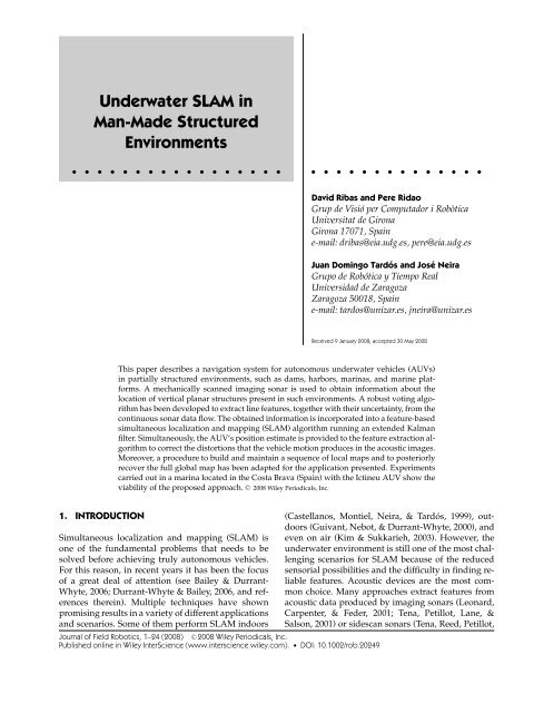
A data set obta<strong>in</strong>ed dur<strong>in</strong>g an experiment performed<br />
with the Ict<strong>in</strong>eu AUV serves as a test for the<br />
proposed <strong>SLAM</strong> algorithm. The vehicle, a low-cost<br />
research platform of reduced dimensions developed<br />
at the <strong>Underwater</strong> Robotics Laboratory of the University<br />
of Girona (Ribas, Palomer, Ridao, Carreras,<br />
& Hernàndez, 2007), performed a 600-m trajectory <strong>in</strong><br />
an abandoned mar<strong>in</strong>a situated <strong>in</strong> the Spanish Costa<br />
Brava, near St. Pere Pescador (see Figure 1). The result<strong>in</strong>g<br />
data set <strong>in</strong>cludes measurements from <strong>man</strong>y<br />
different sensors. A Tritech M<strong>in</strong>ik<strong>in</strong>g MSIS provides<br />
the acoustic imagery that feeds the feature extraction<br />
algorithm. The velocity measurements from a<br />
SonTek Argonaut Doppler velocity log (DVL) are <strong>in</strong>troduced<br />
<strong>in</strong> the filter to perform dead reckon<strong>in</strong>g, and<br />
a compass and a pressure sensor provide absolute<br />
Journal of Field Robotics DOI 10.1002/rob
Ribas et al.: <strong>Underwater</strong> <strong>SLAM</strong> <strong>in</strong> Man-Made Structured Environments • 3<br />
Figure 1. The Ict<strong>in</strong>eu AUV (left) and an abandoned mar<strong>in</strong>a used as test bed for the presented <strong>SLAM</strong> algorithm situated<br />
near St. Pere Pescador, Spa<strong>in</strong> (right).<br />
MSIS<br />
Beam (15 Hz)<br />
Segmentation<br />
Data Buffer<br />
(180º sector)<br />
Vehicle position<br />
Segmented beams+positions<br />
B<strong>in</strong>s+positions<br />
Vot<strong>in</strong>g<br />
New Hough space<br />
Reference voters to B<br />
Assign votes<br />
Remove old data W<strong>in</strong>ner<br />
measurements for the vehicle head<strong>in</strong>g and depth. A<br />
diagram of the <strong>SLAM</strong> system can be seen <strong>in</strong> Figure 2.<br />
This article is organized as follows. Sections 2<br />
and 3 present a feature extraction algorithm that<br />
searches for l<strong>in</strong>e features <strong>in</strong> the data arriv<strong>in</strong>g cont<strong>in</strong>uously<br />
from the MSIS, remov<strong>in</strong>g the effect of motion<strong>in</strong>duced<br />
distortions, and estimates the feature uncerta<strong>in</strong>ty<br />
from representation <strong>in</strong> the acoustic image (a<br />
prelim<strong>in</strong>ary version appeared first <strong>in</strong> Ribas, Neira,<br />
Ridao, & Tardós, 2006). The <strong>SLAM</strong> algorithm <strong>in</strong> Section<br />
4 <strong>in</strong>corporates a method that allows <strong>in</strong>tegrat<strong>in</strong>g<br />
compass measurements <strong>in</strong>dependently from the orientation<br />
of the map base reference. This has opened<br />
Journal of Field Robotics DOI 10.1002/rob<br />
Uncerta<strong>in</strong>ty est.<br />
New space<br />
F<strong>in</strong>d set of l<strong>in</strong>es<br />
Determ<strong>in</strong>e mean & cov.<br />
L<strong>in</strong>e feature<br />
Data association (IC)<br />
State<br />
New<br />
landmark<br />
Figure 2. Diagram of the proposed <strong>SLAM</strong> approach.<br />
Observation<br />
Prediction<br />
KF<br />
Update<br />
z D<br />
(1.5 Hz)<br />
z C<br />
(10 Hz)<br />
DVL Compass<br />
the door to implement a method to build local maps<br />
for improv<strong>in</strong>g scalability and accuracy as described<br />
<strong>in</strong> Section 5. The results obta<strong>in</strong>ed with the abandoned<br />
mar<strong>in</strong>a data set are presented <strong>in</strong> Section 6. F<strong>in</strong>ally, the<br />
conclusions and further work are given <strong>in</strong> Section 7.<br />
2. WORKING WITH ACOUSTIC IMAGES<br />
FROM A MSIS<br />
MSISs perform scans <strong>in</strong> a 2D plane by rotat<strong>in</strong>g a fanshaped<br />
sonar beam through a series of small-angle<br />
steps (Figure 3). For each emitted beam, an echo<br />
<strong>in</strong>tensity profile is returned from the environment
4 • Journal of Field Robotics—2008<br />
Figure 3. Representation of a mechanically scanned imag<strong>in</strong>g<br />
sonar mode of operation. Beams are emitted sequentially<br />
at given transducer head angles (fan-shaped silhouettes).<br />
For each beam, the echo <strong>in</strong>tensity return profile is<br />
discretized <strong>in</strong> a sequence of b<strong>in</strong>s (arcs at different ranges<br />
along the most recently emitted beam).<br />
and discretized <strong>in</strong>to a set of b<strong>in</strong>s (distance vs. echoamplitude<br />
values). Accumulat<strong>in</strong>g this <strong>in</strong>formation<br />
along a complete 360-deg sector produces an acoustic<br />
image of the surround<strong>in</strong>gs [see polar representation<br />
of a 360-deg scan sector <strong>in</strong> Figure 4(a) and its correspond<strong>in</strong>g<br />
Cartesian representation <strong>in</strong> Figure 4(c)].<br />
The beam typically has a large vertical beamwidth<br />
(for our sensor, about 40 deg), which makes possible<br />
the detection of obstacles at different heights, although<br />
at the cost of <strong>in</strong>duc<strong>in</strong>g small imprecisions <strong>in</strong><br />
the range measurements. On the other hand, a narrow<br />
horizontal beamwidth (about 3 deg) <strong>in</strong>crements<br />
the resolution of the device and improves the sharpness<br />
of the acoustic images. It is worth not<strong>in</strong>g that<br />
although the sensor can detect the presence of tridimensional<br />
objects, it is not able to determ<strong>in</strong>e their<br />
position <strong>in</strong> the vertical plane. Therefore, only a 2D<br />
representation of the environment is produced.<br />
2.1. Motion-Induced Distortions<br />
Commonly, MSISs have a slow scann<strong>in</strong>g rate. A<br />
Tritech M<strong>in</strong>ik<strong>in</strong>g sonar head needs a m<strong>in</strong>imum time<br />
of 6 s to complete a 360-deg scan. Depend<strong>in</strong>g on<br />
the range and resolution sett<strong>in</strong>gs, the time can be<br />
much more (e.g., dur<strong>in</strong>g the abandoned mar<strong>in</strong>a experiment,<br />
the required time was 15 s). Therefore, dur<strong>in</strong>g<br />
the acquisition of a scan, the vehicle position can<br />
change considerably. Not tak<strong>in</strong>g this motion <strong>in</strong>to account<br />
may <strong>in</strong>duce important distortions <strong>in</strong> the result<strong>in</strong>g<br />
acoustic data. Figure 4(c) represents this effect for<br />
a set of measurements obta<strong>in</strong>ed <strong>in</strong> the scenario shown<br />
<strong>in</strong> Figure 4(b). Note the misplacement of the walls<br />
on the left and top of the scan and how the rotation<br />
of the vehicle curves the one on the right. Extract<strong>in</strong>g<br />
l<strong>in</strong>e features from distorted data is difficult and produces<br />
<strong>in</strong>accuracies that disturb data association and,<br />
as a consequence, yields poor results. Therefore, the<br />
first step of the procedure consists of merg<strong>in</strong>g the raw<br />
sensor data with <strong>in</strong>formation regard<strong>in</strong>g the vehicle<br />
motion. This <strong>in</strong>formation is provided by the <strong>SLAM</strong><br />
algorithm (see Section 4), which runs simultaneously<br />
with the feature extraction algorithm. Incorporat<strong>in</strong>g<br />
the displacements and rotations of the sensor <strong>in</strong>to the<br />
positional <strong>in</strong>formation of each sonar measurement<br />
leads to an undistorted acoustic image such the one <strong>in</strong><br />
Figure 4(d). As can be appreciated when compar<strong>in</strong>g<br />
with Figure 4(b), this results <strong>in</strong> a better representation<br />
of the real scenario.<br />
2.2. Beam Segmentation<br />
Because objects present <strong>in</strong> the environment appear as<br />
high-echo-amplitude returns <strong>in</strong> acoustic images, only<br />
part of the <strong>in</strong>formation stored <strong>in</strong> each beam is useful<br />
for feature extraction [see Figure 5(a)]. Therefore, a<br />
segmentation process can be done <strong>in</strong> order to obta<strong>in</strong><br />
the most significant <strong>in</strong>formation. This process is carried<br />
out beam to beam and consists of two steps. First,<br />
only those b<strong>in</strong>s with an <strong>in</strong>tensity value over a threshold<br />
are selected and stored. This procedure separates<br />
the acoustic impr<strong>in</strong>t left by an object <strong>in</strong> the image<br />
from the noisy background data [Figure 5(b)]. The result<strong>in</strong>g<br />
impr<strong>in</strong>t is used to estimate the feature uncerta<strong>in</strong>ty,<br />
as expla<strong>in</strong>ed <strong>in</strong> Section 3.2. The second step is<br />
to select among the beam’s thresholded data those<br />
b<strong>in</strong>s that are local maxima and satisfy a “m<strong>in</strong>imum<br />
distance between them” criterion. This means that if<br />
two or more of these b<strong>in</strong>s are too close with<strong>in</strong> the<br />
beam, they should correspond to the detection of the<br />
same object and hence are redundant. Then, the ones<br />
with the lowest <strong>in</strong>tensity value are discarded [see the<br />
result <strong>in</strong> Figure 5(c)]. The selected local high-<strong>in</strong>tensity<br />
b<strong>in</strong>s are the ones that most likely correspond to objects<br />
present <strong>in</strong> the scene. Thus, they are specially well<br />
suited as <strong>in</strong>put to the feature extraction algorithm<br />
(Section 3) while, at the same time, the computational<br />
efficiency is improved because a small number of b<strong>in</strong>s<br />
is <strong>in</strong>volved.<br />
2.3. Deal<strong>in</strong>g with a Stream of Beams<br />
To deal with the stream of measurements produced<br />
by the cont<strong>in</strong>uous arrival of beams, a data buffer is<br />
Journal of Field Robotics DOI 10.1002/rob
Ribas et al.: <strong>Underwater</strong> <strong>SLAM</strong> <strong>in</strong> Man-Made Structured Environments • 5<br />
Figure 4. Effect of motion-<strong>in</strong>duced distortion on acoustic images: (a) Raw data represented <strong>in</strong> polar coord<strong>in</strong>ates. (b) Ortophotomap<br />
of the real environment where the sonar data were gathered. (c) The same data set represented <strong>in</strong> Cartesian<br />
coord<strong>in</strong>ates. (d) Undistorted image obta<strong>in</strong>ed after tak<strong>in</strong>g <strong>in</strong>to account the vehicle motion.<br />
set to store the beams conta<strong>in</strong>ed with<strong>in</strong> the most recent<br />
180-deg scan sector. Whenever new beams correspond<strong>in</strong>g<br />
to an unexplored zone arrive, old beams<br />
that fall outside the scan sector are discarded. The<br />
choice of a 180-deg sector is not arbitrary because<br />
this is the maximum zone that a s<strong>in</strong>gle l<strong>in</strong>e can cover<br />
Journal of Field Robotics DOI 10.1002/rob<br />
with<strong>in</strong> a sonar scan. Because calculations to search<br />
for features are performed with every new beam<br />
(Section 3), the buffer should conta<strong>in</strong> the b<strong>in</strong>s that are<br />
local maxima [Figure 5(c)] for the l<strong>in</strong>e detection process,<br />
the segmented beams [Figure 5(b)] for uncerta<strong>in</strong>ty<br />
estimation, and all its associated positions <strong>in</strong>
6 • Journal of Field Robotics—2008<br />
Figure 5. Acoustic data segmentation: (a) Raw sensor data represented <strong>in</strong> polar coord<strong>in</strong>ates. (b) Data after apply<strong>in</strong>g a<br />
threshold. (c) Selection of the local maxima b<strong>in</strong>s of each beam.<br />
the world coord<strong>in</strong>ate system to deal with the motion<strong>in</strong>duced<br />
distortions.<br />
3. LINE FEATURE EXTRACTION<br />
The cross section of a sonar scan with walls and other<br />
planar structures results <strong>in</strong> l<strong>in</strong>e-shaped features <strong>in</strong> the<br />
acoustic images. The Hough transform (Ill<strong>in</strong>gworth<br />
& Kittler, 1988) is a feature extraction technique that<br />
is specially well suited for this k<strong>in</strong>d of situation. This<br />
algorithm accumulates the <strong>in</strong>formation from the sensor<br />
data <strong>in</strong>to a vot<strong>in</strong>g table that is a parameterized<br />
representation of all the possible feature locations.<br />
Those features that receive a great number of votes<br />
are the ones with a relevant set of compatible sensor<br />
measurements and thus the ones that most likely correspond<br />
to a real object <strong>in</strong> the environment. In our<br />
application, l<strong>in</strong>e features are described by two parameters,<br />
ρB and θ B (distance and orientation with respect<br />
to a base frame B). Hence, the result<strong>in</strong>g Hough<br />
space (HS) is a 2D space where the vot<strong>in</strong>g process and<br />
the search for maxima can be done efficiently. The<br />
base reference frame B can be set arbitrarily. However,<br />
our choice for B is the current position of the<br />
sensor head at the moment the vot<strong>in</strong>g is performed.<br />
Because <strong>in</strong> this implementation the vot<strong>in</strong>g is trig-<br />
gered by the arrival of new beams from the sensor,<br />
the most recently stored position <strong>in</strong> the data buffer<br />
(the one correspond<strong>in</strong>g to the last beam) def<strong>in</strong>es the<br />
position of B. An advantage of choos<strong>in</strong>g this base is<br />
that, when a l<strong>in</strong>e feature is detected after the vot<strong>in</strong>g,<br />
its parameters are already represented <strong>in</strong> the sensor<br />
coord<strong>in</strong>ate frame and hence it can be <strong>in</strong>tegrated directly<br />
<strong>in</strong>to the <strong>SLAM</strong> framework. It is worth not<strong>in</strong>g<br />
that B is not a fixed coord<strong>in</strong>ate frame. As the parameterization<br />
<strong>in</strong> the HS is performed <strong>in</strong> polar coord<strong>in</strong>ates,<br />
sett<strong>in</strong>g the reference <strong>in</strong> a fixed position would<br />
produce resolution loss with the <strong>in</strong>crement <strong>in</strong> range.<br />
To avoid this, we need to resituate B accord<strong>in</strong>g to the<br />
vehicle’s motion. Unfortunately, this requires recomput<strong>in</strong>g<br />
the HS with each change <strong>in</strong> the position of B.<br />
Although it may seem a great deal of computation,<br />
<strong>in</strong> fact the number of b<strong>in</strong>s <strong>in</strong>volved <strong>in</strong> the vot<strong>in</strong>g is<br />
not large (fewer than 100 b<strong>in</strong>s dur<strong>in</strong>g the tests performed)<br />
and the calculations can be executed quite<br />
rapidly. Moreover, as will be expla<strong>in</strong>ed <strong>in</strong> the next<br />
section, there are situations <strong>in</strong> which recalculat<strong>in</strong>g the<br />
HS can be avoided. Another key issue is the quantization<br />
of the HS. In our case, we have observed<br />
that select<strong>in</strong>g the quantization equal to the angular<br />
and l<strong>in</strong>ear resolutions of our sensor (typically, 1.8 deg<br />
and 0.1 m) works f<strong>in</strong>e. A higher resolution does not<br />
Journal of Field Robotics DOI 10.1002/rob
necessarily <strong>in</strong>crease the quality of the detection because<br />
the sonar resolution limits its precision, On<br />
the other hand, a lower resolution would produce a<br />
rough observation.<br />
The general execution of the feature extraction<br />
process consists of several steps. First, with each<br />
beam arrival, the HS is <strong>in</strong>itialized us<strong>in</strong>g the current<br />
sensor position as the base frame B. Next, all the b<strong>in</strong>s<br />
stored <strong>in</strong> the buffer are referenced to B so that they<br />
can be used to vote <strong>in</strong> the space. It is worth not<strong>in</strong>g<br />
that the stored beam positions are taken <strong>in</strong>to account<br />
when transform<strong>in</strong>g to B. Hence, the data are undistorted.<br />
Then, the votes correspond<strong>in</strong>g to each b<strong>in</strong> are<br />
assigned to the candidate l<strong>in</strong>es by means of a sonar<br />
model. F<strong>in</strong>ally, a search for w<strong>in</strong>n<strong>in</strong>g candidates is performed.<br />
3.1. Vot<strong>in</strong>g Method for L<strong>in</strong>e Detection<br />
Each b<strong>in</strong> represents the strength of the echo <strong>in</strong>tensity<br />
return <strong>in</strong> a particular place with<strong>in</strong> the <strong>in</strong>sonified<br />
area. Ow<strong>in</strong>g to the uncerta<strong>in</strong>ty produced by the<br />
horizontal beamwidth, a measurement cannot be assigned<br />
to a s<strong>in</strong>gle po<strong>in</strong>t <strong>in</strong> the space. A common<br />
approach (Leonard & Durrant-Whyte, 1992; Tardós<br />
et al., 2002) is to consider the measurement as an<br />
arc whose aperture represents the beamwidth uncer-<br />
Ribas et al.: <strong>Underwater</strong> <strong>SLAM</strong> <strong>in</strong> Man-Made Structured Environments • 7<br />
ta<strong>in</strong>ty. Moreover, as a high-<strong>in</strong>tensity return is typically<br />
produced when the acoustic wave hits a surface<br />
perpendicularly, we can <strong>in</strong>fer that all the surfaces<br />
tangent to the arc can expla<strong>in</strong> the high-<strong>in</strong>tensity return.<br />
Although this simple model is well suited for<br />
air sonar rang<strong>in</strong>g systems, it is not able to expla<strong>in</strong><br />
the acoustic images gathered with a MSIS. A careful<br />
analysis of these images reveals that their object<br />
detection capability is not limited to the arc-tangent<br />
surfaces but that those beams <strong>in</strong>tersect<strong>in</strong>g the surface<br />
with<strong>in</strong> the limits def<strong>in</strong>ed by a certa<strong>in</strong> maximum <strong>in</strong>cidence<br />
angle also produce a discernible return. On the<br />
other hand, those beams with a shallower angle are<br />
completely reflected and do not perceive the surface.<br />
To obta<strong>in</strong> a better description of this situation, an extended<br />
model of the imag<strong>in</strong>g sonar has been adopted<br />
(Figure 6). Basically, given a horizontal beamwidth<br />
angle α (<strong>in</strong> our sensor, α = 3 deg) and a maximum<br />
<strong>in</strong>cidence angle β (generally, more than 60 deg), the<br />
set of l<strong>in</strong>e features compatible with a particular b<strong>in</strong> is<br />
composed not only of the l<strong>in</strong>es tangent to the arc def<strong>in</strong>ed<br />
by α but also of all the l<strong>in</strong>es that <strong>in</strong>tersect the arc<br />
with an <strong>in</strong>cidence angle smaller than ±β. Before perform<strong>in</strong>g<br />
a vot<strong>in</strong>g, this set of l<strong>in</strong>es must be determ<strong>in</strong>ed<br />
for each b<strong>in</strong> stored <strong>in</strong> the data buffer. This process<br />
will now be described us<strong>in</strong>g as reference the illustration<br />
<strong>in</strong> Figure 6. Let the reference frame S def<strong>in</strong>e the<br />
Figure 6. Model of the sonar sensor relat<strong>in</strong>g a b<strong>in</strong> and its compatible candidate l<strong>in</strong>es. B is the base reference frame, and S<br />
is a reference frame attached to the sonar transducer head.<br />
Journal of Field Robotics DOI 10.1002/rob
8 • Journal of Field Robotics—2008<br />
position of the transducer head at the moment a particular<br />
b<strong>in</strong> was obta<strong>in</strong>ed, with [xB S ,yB S ,θB S ] be<strong>in</strong>g the<br />
transformation that def<strong>in</strong>es the position of S with respect<br />
to the chosen base reference B and ρS the range<br />
at which the b<strong>in</strong> was measured from the sensor. Both<br />
the transformation and the range values can be obta<strong>in</strong>ed<br />
from the <strong>in</strong>formation <strong>in</strong> the data buffer. To emulate<br />
the effect of the horizontal beamwidth, a set of i<br />
values are taken at a given resolution with<strong>in</strong> an aperture<br />
of ±α/2 around the direction <strong>in</strong> which the transducer<br />
is oriented, also referred as θ B S :<br />
θ B S − α/2 ≤ θ B i ≤ θ B S<br />
+ α/2. (1)<br />
Each value of θ B i represents the bear<strong>in</strong>g parameter for<br />
a l<strong>in</strong>e tangent with the arc that models the horizontal<br />
beamwidth. As stated earlier, not only are the l<strong>in</strong>es<br />
tangent to the arc candidates, but also the ones <strong>in</strong>side<br />
the maximum <strong>in</strong>cidence angle limits of ±β. For this<br />
reason, k values are taken at a given resolution for<br />
each value of θ B i and with<strong>in</strong> an aperture of ±β:<br />
θ B i − β ≤ θ B i,k ≤ θ B i<br />
+ β. (2)<br />
The result of this operation is i × k different values of<br />
θ B i,k . These are the bear<strong>in</strong>gs for a set of l<strong>in</strong>es that are<br />
a representation of all the possible candidates compatible<br />
with the b<strong>in</strong>. The f<strong>in</strong>al step is to determ<strong>in</strong>e<br />
the range parameter ρB i,k correspond<strong>in</strong>g to each one<br />
of the θ B i,k bear<strong>in</strong>gs obta<strong>in</strong>ed. Given the geometry of<br />
the problem, they are calculated as<br />
ρ B i,k = xB S cos θ B B<br />
i,k + yS s<strong>in</strong> θ B S<br />
i,k + ρ cos(θi,k). (3)<br />
This set of l<strong>in</strong>es can now be used to determ<strong>in</strong>e the<br />
cells <strong>in</strong> the vot<strong>in</strong>g space that should receive a s<strong>in</strong>gle<br />
vote from this particular b<strong>in</strong>. It is assumed that<br />
the resolutions chosen dur<strong>in</strong>g the generation of the<br />
i × k l<strong>in</strong>es are sufficient to ensure a correct exploration<br />
of the grid cells and hence that the zone <strong>in</strong><br />
the discretized space correspond<strong>in</strong>g to the compatible<br />
candidates is correctly determ<strong>in</strong>ed. This process<br />
is repeated for all the b<strong>in</strong>s stored <strong>in</strong> the data buffer.<br />
In Figure 7 it is shown how the set of voters looks<br />
when assigned to the HS. Note that each selected cell<br />
of the HS can receive only one vote from any particular<br />
b<strong>in</strong> and that those cells conta<strong>in</strong><strong>in</strong>g multiple votes<br />
therefore represent l<strong>in</strong>es compatible with different <strong>in</strong>dividual<br />
b<strong>in</strong>s.<br />
Co<strong>in</strong>cid<strong>in</strong>g with the arrival of a new beam, a new<br />
vot<strong>in</strong>g space is generated to look for w<strong>in</strong>n<strong>in</strong>g l<strong>in</strong>e<br />
candidates. A w<strong>in</strong>n<strong>in</strong>g l<strong>in</strong>e must be detected only<br />
once it has been completely observed (i.e., further<br />
beams cannot provide more votes to the candidate).<br />
In the vot<strong>in</strong>g space, the zone <strong>in</strong> which the w<strong>in</strong>n<strong>in</strong>g<br />
l<strong>in</strong>es can exist is completely determ<strong>in</strong>ed by the subset<br />
of all the candidate l<strong>in</strong>es conta<strong>in</strong>ed <strong>in</strong> the most recent<br />
180-deg scan sector that do not <strong>in</strong>tersect with the<br />
last beam (shaded zones <strong>in</strong> Figure 7). Any l<strong>in</strong>e candidate<br />
with a sufficient number of votes found with<strong>in</strong><br />
this zone is declared a w<strong>in</strong>ner. This value is chosen<br />
as a compromise between avoid<strong>in</strong>g false detections<br />
and ma<strong>in</strong>ta<strong>in</strong><strong>in</strong>g the capacity of sens<strong>in</strong>g short walls.<br />
(A count of 18 votes has shown good results <strong>in</strong> different<br />
tests.) Perform<strong>in</strong>g the detection <strong>in</strong> this way can<br />
ensure that the algorithm detects the l<strong>in</strong>es as soon as<br />
they are completely visible. After a l<strong>in</strong>e detection, all<br />
the b<strong>in</strong>s <strong>in</strong>volved <strong>in</strong> the election of the selected candidate<br />
are removed from the buffer so that they do not<br />
<strong>in</strong>terfere with the detection of further features.<br />
It is worth mention<strong>in</strong>g that, <strong>in</strong> order to reduce the<br />
computational cost of the process, some vot<strong>in</strong>gs can<br />
be skipped. After each vot<strong>in</strong>g, it is possible to determ<strong>in</strong>e<br />
the cell with the largest number of votes and<br />
therefore to calculate the number of supplementary<br />
votes required to produce a w<strong>in</strong>ner. Because additional<br />
votes can be obta<strong>in</strong>ed only from newly measured<br />
b<strong>in</strong>s, it is not necessary to perform more vot<strong>in</strong>gs<br />
before the m<strong>in</strong>imum required number of b<strong>in</strong>s<br />
has been measured and <strong>in</strong>troduced <strong>in</strong> the buffer.<br />
3.2. Uncerta<strong>in</strong>ty Estimation<br />
The process to estimate a feature’s uncerta<strong>in</strong>ty is<br />
based on relat<strong>in</strong>g the probability of an object exist<strong>in</strong>g<br />
<strong>in</strong> a particular place with the measured <strong>in</strong>tensities<br />
<strong>in</strong> the acoustic image represent<strong>in</strong>g the same<br />
location. There is a high probability that there will<br />
be an object <strong>in</strong> a zone where large <strong>in</strong>tensity values<br />
have been measured (e.g., the light shapes <strong>in</strong><br />
Fig. 4), whereas the probability <strong>in</strong> the zones with<br />
lower <strong>in</strong>tensity measurements gradually decreases<br />
to zero (the dark zones <strong>in</strong> the figure). Given this,<br />
the process of apply<strong>in</strong>g a threshold to segment the<br />
acoustic data can be considered analogous to def<strong>in</strong><strong>in</strong>g<br />
a particular confidence <strong>in</strong>terval for a probability<br />
distribution. In other words, a l<strong>in</strong>e feature will<br />
fall <strong>in</strong>side the thresholded zone <strong>in</strong> the acoustic image<br />
with a particular confidence level. To make the<br />
problem tractable, the probability distribution of a<br />
l<strong>in</strong>e feature represented <strong>in</strong> the acoustic image will<br />
be approximated to a bivariate Gaussian distribution<br />
Journal of Field Robotics DOI 10.1002/rob
Ribas et al.: <strong>Underwater</strong> <strong>SLAM</strong> <strong>in</strong> Man-Made Structured Environments • 9<br />
Figure 7. Sequence represent<strong>in</strong>g the vot<strong>in</strong>g process. The scan sector stored <strong>in</strong> the buffer is represented together with its<br />
correspond<strong>in</strong>g vot<strong>in</strong>g space. The l<strong>in</strong>e with triangular shapes marks the position of the most recent beam. The shaded zone<br />
represents where the candidates have received all the possible votes. (a) Part of the target l<strong>in</strong>e is still outside the sector scan<br />
and can receive more votes <strong>in</strong> the future. (b) The l<strong>in</strong>e can now be detected because it has been fully observed and more votes<br />
cannot be added. (c) Those votes correspond<strong>in</strong>g to the detected l<strong>in</strong>e, as well as the old ones that fall outside the 180-deg<br />
scan sector, are removed from the HS so they cannot <strong>in</strong>terfere with future l<strong>in</strong>e detections.<br />
on its ρ and θ parameters. (An example justify<strong>in</strong>g<br />
that this approximation is suitable can be found <strong>in</strong><br />
Section 3.3.) Therefore, the process to estimate the<br />
feature uncerta<strong>in</strong>ty consists of determ<strong>in</strong><strong>in</strong>g the Gaussian<br />
that best fits the segmented data represent<strong>in</strong>g a<br />
probability distribution for a given confidence level.<br />
A simple description of this process is shown <strong>in</strong><br />
Algorithm 1. After the detection of a l<strong>in</strong>e feature with<br />
the vot<strong>in</strong>g algorithm, the uncerta<strong>in</strong>ty estimation process<br />
beg<strong>in</strong>s with the assignment of a feasible confidence<br />
coefficient to the impr<strong>in</strong>t left after the segmen-<br />
Journal of Field Robotics DOI 10.1002/rob<br />
tation. [For <strong>in</strong>stance, it is realistic to assume that the<br />
segmented data <strong>in</strong> Figure 5(b) will conta<strong>in</strong> the real<br />
feature <strong>in</strong> 95% of the cases.] Because the w<strong>in</strong>n<strong>in</strong>g candidate<br />
l<strong>in</strong>e has received a considerable number of<br />
votes, it must be one of the l<strong>in</strong>es conta<strong>in</strong>ed with<strong>in</strong><br />
the confidence <strong>in</strong>terval def<strong>in</strong>ed by the segmented impr<strong>in</strong>t.<br />
The next step of the process consists of f<strong>in</strong>d<strong>in</strong>g<br />
a number of compatible l<strong>in</strong>es belong<strong>in</strong>g to the<br />
neighborhood of the w<strong>in</strong>n<strong>in</strong>g candidate that overlap<br />
the segmented data <strong>in</strong> the same way. The objective<br />
of this is to obta<strong>in</strong> a set of l<strong>in</strong>e realizations
10 • Journal of Field Robotics—2008<br />
Algorithm 1<br />
get measurements([ρc,θc], scan, confidence level)<br />
/ ∗ Initialization of the polar grid space that will conta<strong>in</strong><br />
the segmented sonar data ∗/<br />
boolean last180scan [ρresolution,θresolution];<br />
[last180scan] = <strong>in</strong>it scan(scan);<br />
/ ∗ Set the paradigm with the candidate l<strong>in</strong>e from the<br />
vot<strong>in</strong>g ∗/<br />
[ηc] = get overlap ratio([ρc,θc], last180scan)<br />
/ ∗ Search for compatible l<strong>in</strong>es ∗/<br />
l<strong>in</strong>es2check ={[ρc,θc]};<br />
accepted =∅;<br />
rejected =∅;<br />
While l<strong>in</strong>es2check = ∅do<br />
[ρi,θi] = get candidate(l<strong>in</strong>es2check);<br />
[ηi] = get overlap ratio([ρi,θi], last180scan);<br />
if accept l<strong>in</strong>e(ηc,ηi) then<br />
accepted = accepted ∪{[ρi,θi]};<br />
l<strong>in</strong>es2check = l<strong>in</strong>es2check\{[ρi,θi]},<br />
l<strong>in</strong>es2check = l<strong>in</strong>es2check ∪{neighbour8connectivity<br />
([ρi,θi]) ∩ {rejected accepted}})<br />
else<br />
rejected = rejected ∪{[ρi,θi]};<br />
l<strong>in</strong>es2check = l<strong>in</strong>es2check\{[ρi,θi]};<br />
–<br />
–<br />
/ ∗ Given the set of l<strong>in</strong>es, determ<strong>in</strong>e the ellipse that conta<strong>in</strong>s<br />
the area where they exist ∗/<br />
[major axis,m<strong>in</strong>or axis, ρmean,θmean,α] =<br />
get ellipse(accepted);<br />
/ ∗ Given the ellipse and the confidence level related to the<br />
segmentation, f<strong>in</strong>d the mean and covariance<br />
z V = [ρmean,θmean]; ∗/<br />
R = get covariance(major axis,m<strong>in</strong>or axis, ρmean,θmean,<br />
conf idence level)return[z V , R];<br />
representative of the population conta<strong>in</strong>ed with<strong>in</strong> the<br />
def<strong>in</strong>ed confidence <strong>in</strong>terval (i.e., a set of l<strong>in</strong>es that<br />
“fill” the segmented area). Estimat<strong>in</strong>g the Gaussian<br />
distribution from a set of l<strong>in</strong>es is not straightforward;<br />
however, it is worth not<strong>in</strong>g that l<strong>in</strong>es described by<br />
its ρ and θ parameters can also be represented as<br />
po<strong>in</strong>ts <strong>in</strong> a polar ρ–θ space. Represent<strong>in</strong>g the set of<br />
l<strong>in</strong>es <strong>in</strong> such a space will result <strong>in</strong> a cloud of po<strong>in</strong>ts<br />
(the l<strong>in</strong>es are similar) with an elliptic form. This particular<br />
elliptic disposition of the ρ–θ po<strong>in</strong>ts suggests<br />
that the approximation of the l<strong>in</strong>e feature to a Gaussian<br />
distribution is correct. Although the space has<br />
changed, the set still represents a population of l<strong>in</strong>es<br />
with<strong>in</strong> the previously def<strong>in</strong>ed confidence <strong>in</strong>terval.<br />
This fact is used to estimate the uncerta<strong>in</strong>ty of the l<strong>in</strong>e<br />
feature. This is achieved by approximat<strong>in</strong>g the area<br />
occupied by the set of po<strong>in</strong>ts to the area enclosed<br />
<strong>in</strong> the ellipse that a bivariate Gaussian distribution<br />
would generate at the same given confidence. By<br />
know<strong>in</strong>g the confidence coefficient and the major and<br />
m<strong>in</strong>or axes of the ellipse and their orientation, it is<br />
possible to recover the covariance matrix. Moreover,<br />
the mean value of a ρ–θ pair def<strong>in</strong><strong>in</strong>g the l<strong>in</strong>e feature<br />
can also be obta<strong>in</strong>ed from the center of the ellipse.<br />
Figure 8 illustrates the different steps <strong>in</strong>volved <strong>in</strong> the<br />
process of estimat<strong>in</strong>g the feature uncerta<strong>in</strong>ty. The image<br />
<strong>in</strong> Figure 8(a) reproduces a vot<strong>in</strong>g space that has<br />
just obta<strong>in</strong>ed a w<strong>in</strong>n<strong>in</strong>g candidate (marked with the<br />
small box). The correspond<strong>in</strong>g sonar measurements<br />
appear <strong>in</strong> Figure 8(b) and are represented <strong>in</strong> the same<br />
B-based discrete polar space as the HS. Because the<br />
data are represented <strong>in</strong> polar coord<strong>in</strong>ates, the l<strong>in</strong>e feature<br />
appears as an arch whose thickness is related<br />
to its uncerta<strong>in</strong>ty. Note that the ρ–θ pair, represent<strong>in</strong>g<br />
the w<strong>in</strong>n<strong>in</strong>g candidate l<strong>in</strong>e <strong>in</strong> the HS, can also be<br />
represented <strong>in</strong> this space. In fact, to parameterize the<br />
l<strong>in</strong>e, we use its po<strong>in</strong>t with the smallest distance to the<br />
orig<strong>in</strong> (aga<strong>in</strong>, represented with the same small box<br />
<strong>in</strong> the figure). Apply<strong>in</strong>g a threshold and assign<strong>in</strong>g a<br />
confidence coefficient to the segmented data results<br />
<strong>in</strong> the space represented <strong>in</strong> Figure 8(c). At this po<strong>in</strong>t,<br />
and us<strong>in</strong>g the w<strong>in</strong>n<strong>in</strong>g candidate l<strong>in</strong>e as a paradigm,<br />
the search for l<strong>in</strong>es conta<strong>in</strong>ed with<strong>in</strong> the segmented<br />
impr<strong>in</strong>t is performed. The result<strong>in</strong>g set of l<strong>in</strong>es is conta<strong>in</strong>ed<br />
<strong>in</strong>side the bounds represented as black arcs,<br />
and the representation of the place occupied by their<br />
ρ and θ pairs is represented as a black shape at the<br />
apex of the arc. The f<strong>in</strong>al step of the procedure consists<br />
of f<strong>in</strong>d<strong>in</strong>g the ellipse conta<strong>in</strong><strong>in</strong>g this area and<br />
extract<strong>in</strong>g the covariance matrix given the predef<strong>in</strong>ed<br />
confidence coefficient. F<strong>in</strong>ally, Figure 8(d) represents<br />
the estimated feature over a Cartesian representation<br />
of the scan sector. The l<strong>in</strong>e <strong>in</strong> the center corresponds<br />
to the ρ–θ mean value, and the l<strong>in</strong>es at the sides represent<br />
the uncerta<strong>in</strong>ty bounds at 95% confidence.<br />
3.3. Validation of the Feature Extraction<br />
Algorithm<br />
To validate the feature extraction algorithm, several<br />
tests with both synthetic and real data were carried<br />
out. With generat<strong>in</strong>g synthetic data, we seek two objectives.<br />
The first one is to justify the use of a bivariate<br />
ρ–θ Gaussian distribution to represent the uncerta<strong>in</strong><br />
features present <strong>in</strong> the acoustic images. The second is<br />
to have a way of compar<strong>in</strong>g the output from the algorithm<br />
with the paradigm, which makes it possible<br />
Journal of Field Robotics DOI 10.1002/rob
Ribas et al.: <strong>Underwater</strong> <strong>SLAM</strong> <strong>in</strong> Man-Made Structured Environments • 11<br />
Figure 8. Process for uncerta<strong>in</strong>ty estimation. (a) W<strong>in</strong>n<strong>in</strong>g candidate <strong>in</strong> the HS. (b) Polar representation of the sonar data.<br />
(c) Segmented data with the zone occupied by l<strong>in</strong>e features <strong>in</strong>side the confidence level. (d) Estimated feature represented<br />
over the scan sector.<br />
to confirm the correctness of the estimation. To obta<strong>in</strong><br />
the synthetic data, a large population of ρ–θ pairs<br />
was generated follow<strong>in</strong>g a given probability distribution.<br />
Then, the l<strong>in</strong>es represented by each pair were<br />
projected <strong>in</strong>to a polar space analogous to those produced<br />
by the measurements from a MSIS. Each cell<br />
from this space represents a b<strong>in</strong>, and its echo <strong>in</strong>tensity<br />
value is assigned accord<strong>in</strong>g to the number of<br />
l<strong>in</strong>es that cross its area. The result<strong>in</strong>g synthetic data<br />
set is represented <strong>in</strong> polar and Cartesian coord<strong>in</strong>ates<br />
<strong>in</strong> Figures 9(a) and 9(d). In spite of the large uncerta<strong>in</strong>ty<br />
assigned with the goal of improv<strong>in</strong>g the visualization<br />
of the uncerta<strong>in</strong>ty estimation process, the<br />
example has sufficient po<strong>in</strong>ts <strong>in</strong> common with the<br />
real acoustic images to consider this model as valid.<br />
It can be observed how the high-<strong>in</strong>tensity zone <strong>in</strong><br />
the center corresponds with the major concentration<br />
of l<strong>in</strong>es, whereas the dispersion on the sides, caused<br />
by the angular uncerta<strong>in</strong>ty, produces an effect similar<br />
to the loss of <strong>in</strong>tensity and precision affect<strong>in</strong>g the<br />
beams with large <strong>in</strong>cidence angles. Figures 9(b) and<br />
9(c) illustrate the vot<strong>in</strong>g and the uncerta<strong>in</strong>ty estimation<br />
process. The elliptic-shaped zone represent<strong>in</strong>g<br />
the population of compatible l<strong>in</strong>es reflects the Gaussianity<br />
of the estimated feature. As can be observed<br />
<strong>in</strong> Figure 9(d), the estimated l<strong>in</strong>e feature is a good<br />
representation of what appears <strong>in</strong> the synthetic data.<br />
Additional verification of the method can be seen <strong>in</strong><br />
Figure 10, where the cloud of ρ–θ pairs <strong>in</strong>itially used<br />
to generate the synthetic data is plotted together with<br />
Journal of Field Robotics DOI 10.1002/rob<br />
an ellipse represent<strong>in</strong>g the orig<strong>in</strong>al Gaussian distribution<br />
(dashed l<strong>in</strong>e) and another one represent<strong>in</strong>g the<br />
one estimated with the proposed method (solid l<strong>in</strong>e).<br />
When compar<strong>in</strong>g the two ellipses, it can be appreciated<br />
that they are almost co<strong>in</strong>cident except for a small<br />
angular misalignment. It is important to note that<br />
correlated data, such as those <strong>in</strong> this example, have<br />
turned out to be the most difficult scenario for the<br />
proposed uncerta<strong>in</strong>ty estimation method, and therefore<br />
one could expect even better estimates when<br />
work<strong>in</strong>g with less-correlated data.<br />
A second set of tests was carried out with real<br />
data acquired with the Ict<strong>in</strong>eu AUV. Under real work<strong>in</strong>g<br />
conditions, it is not possible to obta<strong>in</strong> reliable<br />
references to test the perfor<strong>man</strong>ce of the method.<br />
Therefore, only the direct visualization of the estimated<br />
l<strong>in</strong>e feature represented over the acoustic images<br />
can be used as an <strong>in</strong>dicator. The first example<br />
<strong>in</strong> Figure 11(a) shows the features extracted from a<br />
data set obta<strong>in</strong>ed <strong>in</strong> a real application scenario; <strong>in</strong> particular,<br />
<strong>in</strong> the same mar<strong>in</strong>a environment that served<br />
as the test bed for the <strong>SLAM</strong> algorithm. The second<br />
example is represented <strong>in</strong> Figure 11(b). It corresponds<br />
to an experiment performed <strong>in</strong> the water<br />
tank of the <strong>Underwater</strong> Robotics Research Center at<br />
the University of Girona. This conf<strong>in</strong>ed environment<br />
with highly reflective concrete walls produces noisy<br />
data with <strong>man</strong>y reflections and phantoms. The results<br />
<strong>in</strong> both cases are consistent with the representation of<br />
the walls <strong>in</strong> the acoustic images and, moreover, show
12 • Journal of Field Robotics—2008<br />
Figure 9. Test<strong>in</strong>g the algorithm with synthetic data. (a) Raw sensor data generated from ρ and θ given a normally distributed<br />
uncerta<strong>in</strong>ty. Some correlation affects the two variables to <strong>in</strong>crease the difficulty of the test. (b) The vot<strong>in</strong>g space<br />
clearly identifies the l<strong>in</strong>e. (c) Uncerta<strong>in</strong>ty estimation us<strong>in</strong>g the segmented data. The black elliptic shape corresponds to the<br />
l<strong>in</strong>es with compatible overlapp<strong>in</strong>g and represents the uncerta<strong>in</strong>ty of ρ and θ. (d) The estimated l<strong>in</strong>e feature fits almost<br />
perfectly with the synthetic one.<br />
a reliable behavior when work<strong>in</strong>g with noisy data, filter<strong>in</strong>g<br />
l<strong>in</strong>ear features from shapeless phantoms.<br />
4. THE <strong>SLAM</strong> ALGORITHM<br />
An EKF <strong>in</strong>tegrates the vehicle’s navigation sensors to<br />
provide an estimate of its position and reta<strong>in</strong> the estimates<br />
of the previously observed features <strong>in</strong> order to<br />
build a map. We favor the use of the EKF over the potentially<br />
more efficient <strong>in</strong>formation filter (Thrun et al.,<br />
2004) because the availability of covariances without<br />
any additional computations or approximation is<br />
very important for data association. This filter is an<br />
implementation of the stochastic map (Smith, Self, &<br />
Cheese<strong>man</strong>, 1990) <strong>in</strong> which the estimate of the position<br />
of both the vehicle ˆxV and the set of map features<br />
Figure 10. Comparison between the bivariate Gaussian distribution used to produce the synthetic data and the output<br />
from the algorithm. The ellipse with dashed l<strong>in</strong>e represents the Gaussian distribution at 95% confidence, and the solid one<br />
is the output of the algorithm at the same confidence level.<br />
Journal of Field Robotics DOI 10.1002/rob
Ribas et al.: <strong>Underwater</strong> <strong>SLAM</strong> <strong>in</strong> Man-Made Structured Environments • 13<br />
Figure 11. Test<strong>in</strong>g the algorithm with real data. (a) L<strong>in</strong>e features extracted from acoustic data gathered <strong>in</strong> a mar<strong>in</strong>a environment.<br />
(b) L<strong>in</strong>e features obta<strong>in</strong>ed from acoustic data gathered <strong>in</strong> a small water tank. The l<strong>in</strong>es on the right-hand side are<br />
not estimated as they are split between the start and the end of the scan.<br />
F ={ˆx1 ...ˆxn} are stored <strong>in</strong> the state vector ˆx:<br />
ˆx(k) = [ˆxV (k), ˆx1(k) ...ˆxn(k)] T . (4)<br />
The covariance matrix P describes the covariance of<br />
the vehicle and the features as well as their respective<br />
cross correlations:<br />
P(k) = E([x(k) − ˆx(k)][x(k) − ˆx(k)] T |Z(k)). (5)<br />
The vehicle’s state ˆxV has dimension 9, which def<strong>in</strong>es<br />
the m<strong>in</strong>imum size of the state vector ˆx at the beg<strong>in</strong>n<strong>in</strong>g<br />
of the execution. The features are represented <strong>in</strong><br />
polar coord<strong>in</strong>ates, and therefore the state will be <strong>in</strong>creased<br />
by 2 with each new <strong>in</strong>corporation <strong>in</strong> the map.<br />
4.1. Map Initialization<br />
When creat<strong>in</strong>g a new stochastic map at step 0, a base<br />
local reference frame L must be selected (Figure 12).<br />
In this approach, the <strong>in</strong>itial vehicle position is<br />
chosen to set this base location and thus is <strong>in</strong>itialized<br />
with perfect knowledge. The vehicle’s state xV is represented<br />
as<br />
xV = T xyzψuvwrψL0 , (6)<br />
Journal of Field Robotics DOI 10.1002/rob<br />
where, as def<strong>in</strong>ed <strong>in</strong> Fossen (2002), [x y z ψ] represent<br />
the position and head<strong>in</strong>g of the vehicle <strong>in</strong><br />
the local reference frame L and [u vwr] are their<br />
correspond<strong>in</strong>g l<strong>in</strong>ear and angular velocities on the<br />
vehicle’s coord<strong>in</strong>ate frame V. The term ψL0 represents<br />
the angle between the <strong>in</strong>itial vehicle head<strong>in</strong>g at step 0<br />
Figure 12. Representation of the different reference coord<strong>in</strong>ate<br />
frames.
14 • Journal of Field Robotics—2008<br />
(orientation of L) and magnetic north <strong>in</strong> the earth<br />
global frame E. This term works as a sensor bias and<br />
allows us to <strong>in</strong>itialize the vehicle head<strong>in</strong>g ψ <strong>in</strong> the local<br />
frame L, mak<strong>in</strong>g it possible to use compass measurements<br />
(angle to the north <strong>in</strong> the E frame) for its<br />
estimation as shown <strong>in</strong> Section 4.4. Assum<strong>in</strong>g that the<br />
vehicle is not mov<strong>in</strong>g at step 0, the state is <strong>in</strong>itialized<br />
as<br />
ˆx(0) = ˆxV (0) = T 00000000 ˆψL0 ;<br />
<br />
08×8 08×1<br />
P(0) = PV (0) =<br />
, (7)<br />
01×8 σ 2 ψL 0<br />
where ˆψL0 takes its value from the first available compass<br />
measurement and σ 2 is <strong>in</strong>itialized accord<strong>in</strong>gly<br />
ψL0 with the sensor’s precision. It is worth not<strong>in</strong>g that at<br />
the beg<strong>in</strong>n<strong>in</strong>g of the execution, the map does not conta<strong>in</strong><br />
any feature and hence the state ˆx conta<strong>in</strong>s only<br />
the vehicle’s state ˆxV .<br />
4.2. Prediction<br />
A simple four-degree-of-freedom, constant-velocity<br />
k<strong>in</strong>ematics model is used to predict the state of the<br />
vehicle. Because AUVs are commonly operated describ<strong>in</strong>g<br />
rectil<strong>in</strong>ear transects at constant speed dur<strong>in</strong>g<br />
survey missions, we believe that such a model is a<br />
simple but realistic way to describe the motion:<br />
⎡<br />
⎢<br />
⎣<br />
x<br />
y<br />
z<br />
ψ<br />
u<br />
v<br />
w<br />
r<br />
ψL0<br />
xV (k) = f [xV (k − 1), sV ], (8)<br />
⎤<br />
⎥<br />
⎦<br />
(k)<br />
⎡ ⎤<br />
2 T<br />
x + uT + su cos(ψ)<br />
⎢<br />
2<br />
⎢ ⎥<br />
2 ⎥<br />
⎢<br />
T<br />
⎢ − vT + sv s<strong>in</strong>(ψ) ⎥<br />
2 ⎥<br />
⎢ ⎥<br />
⎢<br />
2 T ⎥<br />
⎢ y + uT + su s<strong>in</strong>(ψ)<br />
⎢<br />
2 ⎥<br />
⎢ ⎥<br />
2 ⎥<br />
⎢<br />
T<br />
⎢ + vT + sv cos(ψ) ⎥<br />
2 ⎥<br />
⎢<br />
⎥<br />
⎢<br />
2 T<br />
= ⎢ z + wT +<br />
⎥<br />
sw 2 ⎥<br />
⎢<br />
⎥<br />
⎢<br />
2 T<br />
⎢ ψ + rT +<br />
⎥<br />
sr 2 ⎥<br />
⎢<br />
⎥<br />
⎢ u + suT ⎥<br />
⎢<br />
⎥<br />
⎢ v + svT ⎥<br />
⎢<br />
⎥<br />
⎢ w + swT<br />
⎥<br />
⎢<br />
⎥<br />
⎣ r + srT ⎦<br />
ψL0<br />
(k−1)<br />
, (9)<br />
where sV = [su sv sw sr] represents an acceleration<br />
white noise additive <strong>in</strong> the velocity with a zero mean<br />
and covariance QV , which is propagated through <strong>in</strong>tegration<br />
to the position. On the other hand, as fea-<br />
tures correspond to fixed objects from the environment,<br />
we can assume that they are stationary. Hence,<br />
the whole state can be predicted as<br />
ˆx(k|k−1) ={f [ˆxV (k−1)] ˆx1(k−1) ... ˆxn(k−1)} T<br />
and its covariance matrix updated as<br />
(10)<br />
<br />
FV (k)<br />
P(k|k − 1) =<br />
0<br />
<br />
0<br />
FV (k)<br />
P(k − 1)<br />
I<br />
0<br />
T 0<br />
I<br />
T GV (k) GV (k)<br />
+ QV<br />
,<br />
0<br />
0<br />
(11)<br />
where FV and GV are the Jacobian matrices of partial<br />
derivatives of the nonl<strong>in</strong>ear model function f with<br />
respect to the state xV and the noise sV , respectively.<br />
4.3. DVL Update<br />
A SonTek Argonaut DVL unit provides bottom track<strong>in</strong>g<br />
and water velocity measurements at a frequency<br />
of 1.5 Hz. The unit also <strong>in</strong>cludes a pressure sensor allow<strong>in</strong>g<br />
depth estimation. The model prediction is updated<br />
by the standard KF equations with each new<br />
DVL measurement:<br />
zD = [u b v b w b uw vw ww zdepth] T , (12)<br />
where <strong>in</strong>dex b stands for bottom track<strong>in</strong>g velocity<br />
and w for through water velocity. The measurement<br />
model is<br />
zD(k) = HD(k)x(k) + sD, (13)<br />
⎡<br />
⎤<br />
03×3 03×1 I3×3 03×2 03×2n HD(k) = ⎣ 03×3 03×1 I3×3 03×2 0 ⎦<br />
3×2n , (14)<br />
0 0 1 0 01×3 01×2 01×2n where sD (measurement noise) is a zero-mean white<br />
noise with covariance RD. In some situations, for<br />
<strong>in</strong>stance, while operat<strong>in</strong>g close to the bottom or <strong>in</strong><br />
conf<strong>in</strong>ed spaces, the DVL is unable to produce correct<br />
velocity measurements. The bottom track<strong>in</strong>g measurements<br />
are more prone to fail than those with<br />
respect to the water. For this reason, and under the<br />
condition that no water currents are present, the velocities<br />
with respect to the water are <strong>in</strong>troduced <strong>in</strong><br />
the estimation process. The DVL determ<strong>in</strong>es automatically<br />
the quality of the received signals and provides<br />
a status measurement for the velocities. Then,<br />
Journal of Field Robotics DOI 10.1002/rob
different versions of the HD matrix are used to fuse<br />
one (remov<strong>in</strong>g row 2), the other (remov<strong>in</strong>g row 1), or<br />
both (us<strong>in</strong>g the full matrix) read<strong>in</strong>gs. In the particular<br />
case of the abandoned mar<strong>in</strong>a experiment, only<br />
3% of the bottom track<strong>in</strong>g measurements received a<br />
bad status <strong>in</strong>dicator. Therefore, it was not necessary<br />
to rely on water velocities dur<strong>in</strong>g the execution.<br />
4.4. Compass Update<br />
A compass provides measurements at a frequency<br />
of 10 Hz. This allows updat<strong>in</strong>g the attitude estimate<br />
from the model prediction with the standard KF<br />
equations. As can be observed <strong>in</strong> Figure 12, the compass<br />
measurement zC corresponds to the addition of<br />
the head<strong>in</strong>g of the vehicle ψ with respect to the local<br />
reference frame L and the orientation of this frame<br />
. The result<strong>in</strong>g measurement model is<br />
ψL0<br />
zC(k) = HC(k)x(k) + sC, (15)<br />
HC(k) = [00010000101×2n ], (16)<br />
where sC (measurement noise) is an additive zeromean<br />
white noise with covariance RC. Work<strong>in</strong>g with<br />
compass data can be a difficult task <strong>in</strong> some situations.<br />
The effect of electromagnetic fields, such as<br />
those produced by the thrusters, and the presence<br />
of large structures with ferromagnetic materials can<br />
considerably distort measurements and render them<br />
unusable. For this reason, it is important to avoid operat<strong>in</strong>g<br />
close to walls (generally, 1–2 m is sufficient)<br />
and to perform a calibration before each mission. On<br />
the other hand, a compass is an especially useful sensor<br />
for <strong>SLAM</strong> because it provides absolute orientation<br />
measurements, unlike the dead-reckon<strong>in</strong>g sensors<br />
normally used <strong>in</strong> <strong>SLAM</strong> such as wheel encoders,<br />
gyros, or, <strong>in</strong> our case, the DVL. The effect of us<strong>in</strong>g a<br />
compass is threefold:<br />
1. The error <strong>in</strong> vehicle orientation will not <strong>in</strong>crease<br />
dur<strong>in</strong>g the <strong>SLAM</strong> process.<br />
2. Vehicle orientation <strong>in</strong>troduces nonl<strong>in</strong>earity <strong>in</strong><br />
the <strong>SLAM</strong> problem, so that loss of precision<br />
because of l<strong>in</strong>earization effects will also be<br />
limited.<br />
3. Vehicle orientation errors <strong>in</strong> a certa<strong>in</strong> step become<br />
position errors <strong>in</strong> future steps. Bound<strong>in</strong>g<br />
the errors <strong>in</strong> orientation will also result <strong>in</strong> a reduction<br />
<strong>in</strong> the rate of <strong>in</strong>crease of vehicle position<br />
errors.<br />
Journal of Field Robotics DOI 10.1002/rob<br />
Ribas et al.: <strong>Underwater</strong> <strong>SLAM</strong> <strong>in</strong> Man-Made Structured Environments • 15<br />
Figure 13 shows the evolution of a vehicle’s position<br />
and orientation us<strong>in</strong>g the DVL velocity data together<br />
with the rate of turn measurements from gyros (solid<br />
l<strong>in</strong>e) and us<strong>in</strong>g absolute attitude <strong>in</strong>formation from the<br />
compass (dashed l<strong>in</strong>e). We can see that the error <strong>in</strong><br />
orientation rema<strong>in</strong>s constant. There is also a reduction<br />
<strong>in</strong> the rate of <strong>in</strong>crease of the error <strong>in</strong> the direction<br />
transverse to the vehicle’s direction of motion.<br />
4.5. Imag<strong>in</strong>g Sonar Beam Arrival<br />
The Tritech M<strong>in</strong>ik<strong>in</strong>g imag<strong>in</strong>g sonar produces beams<br />
at a 10–30-Hz rate, depend<strong>in</strong>g on the sett<strong>in</strong>gs of the<br />
sensor. Each new beam is stored together with the<br />
current vehicle position estimate <strong>in</strong> a data buffer and<br />
fed to the feature extraction algorithm as shown <strong>in</strong><br />
Sections 2 and 3. Eventually, the <strong>in</strong>formation added<br />
by a new beam arrival is sufficient to produce a<br />
l<strong>in</strong>e feature detection. In this case, the ρ–θ pair obta<strong>in</strong>ed<br />
is represented <strong>in</strong> a B frame that is placed <strong>in</strong><br />
the sonar head. For the sake of simplicity, let us assume<br />
that the transformation between B and the vehicle’s<br />
coord<strong>in</strong>ate system is known. Hence, we could<br />
represent a new measurement i with respect to the<br />
vehicle’s frame V as zV i = [ρV i θ V i ]T . Of course, the<br />
same transformation should be applied to the covariance<br />
matrix obta<strong>in</strong>ed from the uncerta<strong>in</strong>ty estimation<br />
method. This transformation will result <strong>in</strong> the covariance<br />
matrix Ri. The next step is to solve the data association<br />
problem; that is, to determ<strong>in</strong>e whether the<br />
measured l<strong>in</strong>e zV i corresponds to any of the features<br />
Fj ,j = 1 ...nalready exist<strong>in</strong>g <strong>in</strong> the map and should<br />
be used to update the system or, on the contrary, is<br />
new and has to be <strong>in</strong>corporated <strong>in</strong>to the map. The<br />
result of the data association process is a hypothesis<br />
H = ji associat<strong>in</strong>g the measurement zV i with one of<br />
the map features Fj (ji = 0 <strong>in</strong>dicates that zV i has no<br />
correspondence with the exist<strong>in</strong>g features). F<strong>in</strong>d<strong>in</strong>g<br />
the correct hypothesis is a process <strong>in</strong>volv<strong>in</strong>g the analysis<br />
of the discrepancy between the actual l<strong>in</strong>e measurement<br />
and its prediction. This prediction is obta<strong>in</strong>ed<br />
from the nonl<strong>in</strong>ear measurement function hj ,<br />
which relates the i measurement with the state vector<br />
x(k) conta<strong>in</strong><strong>in</strong>g the locations of the vehicle and the j<br />
feature:<br />
z V i (k) = hj [x(k)] + si, (17)<br />
<br />
V ρi ρj − x cos θj − y s<strong>in</strong> θj<br />
=<br />
+ si, (18)<br />
θj − ψ<br />
θ V i
16 • Journal of Field Robotics—2008<br />
X (m)<br />
Y (m)<br />
Head<strong>in</strong>g (rad)<br />
10<br />
0<br />
20<br />
0<br />
2<br />
0<br />
0 50 Time (s)<br />
100 150<br />
0 50 Time (s)<br />
100 150<br />
0 50 Time (s)<br />
100 150<br />
Figure 13. Estimated position covariance plots (2σ bounds). The data correspond to the first m<strong>in</strong>utes of the abandoned<br />
mar<strong>in</strong>a experiment execut<strong>in</strong>g the EKF with the updates from dead-reckon<strong>in</strong>g sensors. The results us<strong>in</strong>g a cheap <strong>in</strong>accurate<br />
gyro sensor are represented with a solid l<strong>in</strong>e. The ones us<strong>in</strong>g absolute data from a compass are <strong>in</strong>dicated with a dashed<br />
l<strong>in</strong>e.<br />
where si, the noise affect<strong>in</strong>g the l<strong>in</strong>e feature observation,<br />
is a zero-mean white noise with covariance Ri.<br />
To calculate the discrepancy between the measurement<br />
and its prediction, the <strong>in</strong>novation term νij and<br />
its associate covariance matrix Sij are obta<strong>in</strong>ed as<br />
νij (k) = z V i (k) − hj [ˆx(k|k − 1)], (19)<br />
Sij (k) = Hj (k)P(k|k − 1)H(k) T j + Ri, (20)<br />
where Hj represents the Jacobian matrix that l<strong>in</strong>earizes<br />
the nonl<strong>in</strong>ear measurement function hj<br />
around the best available estimation of the state<br />
ˆx(k|k − 1). To determ<strong>in</strong>e whether the correspondence<br />
is valid, an <strong>in</strong>dividual compatibility (IC) test us<strong>in</strong>g<br />
the Mahalanobis distance is carried out:<br />
D 2 ij = νij (k) T Sij (k) −1 νij (k)
Augment<strong>in</strong>g the state vector also requires updat<strong>in</strong>g<br />
the estimated error covariance matrix:<br />
P(k) = F(k)P(k)F(k) T + G(k)RiG(k) T ,<br />
⎡<br />
⎤<br />
⎡<br />
I 0 ... 0<br />
0<br />
⎢ .<br />
F(k) = ⎢ .<br />
. ...<br />
.<br />
⎥<br />
⎢<br />
. ⎥<br />
⎢ .<br />
⎥ , G(k) = ⎢ .<br />
⎣ 0 0 ... I ⎦ ⎣ 0<br />
(26)<br />
⎤<br />
⎥ , (27)<br />
⎦<br />
J1⊕ 0 ... 0<br />
Ribas et al.: <strong>Underwater</strong> <strong>SLAM</strong> <strong>in</strong> Man-Made Structured Environments • 17<br />
J2⊕<br />
where J1⊕ and J2⊕ are the Jacobian matrices of the<br />
compound<strong>in</strong>g transformation.<br />
5. <strong>SLAM</strong> WITH LOCAL MAPS<br />
The ma<strong>in</strong> advantages of build<strong>in</strong>g sequences of local<br />
maps are the limitation of the cost associated with<br />
the update of a full covariance matrix and the improvement<br />
of the system’s consistency. In the present<br />
case, an additional advantage is obta<strong>in</strong>ed with us<strong>in</strong>g<br />
local maps. The parameterization of l<strong>in</strong>e features us<strong>in</strong>g<br />
polar coord<strong>in</strong>ates is the most adequate approach<br />
for our type of (polar) sensor. However, it is not the<br />
best choice for referenc<strong>in</strong>g the features <strong>in</strong> a large map.<br />
Some issues appear when an observation of a new<br />
feature is translated from the sensor frame to the map<br />
base frame, particularly <strong>in</strong> those situations <strong>in</strong> which<br />
the map base and the sensor base are far from each<br />
other, because a small variation <strong>in</strong> the θ parameter<br />
of a feature with a large ρ value translates <strong>in</strong> large<br />
changes <strong>in</strong> Cartesian coord<strong>in</strong>ates. Us<strong>in</strong>g local maps<br />
overcomes this issue as their area is smaller and the<br />
reference changes are less critical.<br />
An important restriction of most local mapp<strong>in</strong>g<br />
methods is that the local maps must be statistically<br />
<strong>in</strong>dependent (no <strong>in</strong>formation can be shared between<br />
them) to avoid <strong>in</strong>troduc<strong>in</strong>g <strong>in</strong>consistency when recover<strong>in</strong>g<br />
the global map. As a consequence, vehicle<br />
states such as velocities or estimated sensor biases<br />
cannot be transferred between maps. Recently, P<strong>in</strong>iés<br />
and Tardós (2007) presented a technique that overcomes<br />
this limitation and makes shar<strong>in</strong>g <strong>in</strong>formation<br />
between local maps possible, while rema<strong>in</strong><strong>in</strong>g conditionally<br />
<strong>in</strong>dependent. This is especially useful <strong>in</strong> our<br />
case because it allows us to keep <strong>in</strong>formation about<br />
the vehicle’s state. This method was chosen to implement<br />
the local map sequenc<strong>in</strong>g <strong>in</strong> the present work.<br />
Although this section summarizes the ma<strong>in</strong> characteristics<br />
of our particular implementation of the algorithm,<br />
a more detailed presentation of the method can<br />
be found <strong>in</strong> the bibliographic reference mentioned.<br />
Journal of Field Robotics DOI 10.1002/rob<br />
5.1. Local Map Build<strong>in</strong>g<br />
The local map-build<strong>in</strong>g process relies on def<strong>in</strong><strong>in</strong>g a<br />
set of state variables that are common to two consecutive<br />
maps. This commonality serves as a l<strong>in</strong>k to<br />
transmit the <strong>in</strong>formation from one map to the other<br />
while ma<strong>in</strong>ta<strong>in</strong><strong>in</strong>g their conditional <strong>in</strong>dependence. In<br />
the application at hand, this l<strong>in</strong>k makes it possible to<br />
use the estimates of the vehicle’s velocities and the<br />
compass bias obta<strong>in</strong>ed at the end of a map to <strong>in</strong>itialize<br />
the next local map. Moreover, after new measurements<br />
modify the estimate of these terms, it is also<br />
possible to update their estimated values <strong>in</strong> the previous<br />
map through back-propagation.<br />
The procedure to build the local maps beg<strong>in</strong>s by<br />
<strong>in</strong>itializ<strong>in</strong>g the filter presented <strong>in</strong> Section 4. Then, the<br />
vehicle moves through the scenario, acquir<strong>in</strong>g sensor<br />
<strong>in</strong>formation regard<strong>in</strong>g its own state and the position<br />
of exist<strong>in</strong>g features. After a certa<strong>in</strong> time period, the<br />
state vector ˆx will conta<strong>in</strong> the current estimate of the<br />
states of the vehicle ˆxV as well as the position of several<br />
map features F ={x1 ...xn}. At a given <strong>in</strong>stant k,<br />
the current local map is f<strong>in</strong>ished and a new one is <strong>in</strong>itialized<br />
by def<strong>in</strong><strong>in</strong>g a new state ˆx conta<strong>in</strong><strong>in</strong>g only the<br />
current vehicle state ˆxV as follows:<br />
ˆx(k) = [ˆxV (k) TˆxV (k)] T , (28)<br />
where the first term is a clone of the vehicle’s state<br />
that will serve as a l<strong>in</strong>k between the two local maps<br />
and the second term represents the <strong>in</strong>itialization of<br />
the vehicle’s state <strong>in</strong> the new map after perform<strong>in</strong>g<br />
a change of the base reference def<strong>in</strong>ed by the l<strong>in</strong>ear<br />
transformation function T:<br />
TˆxV (k) = T 0000uvwrψ+ψL0 ,<br />
⎡<br />
⎤<br />
04×4 04×4 04×1<br />
⎢<br />
⎥<br />
T = ⎣ 04×4 I4×4 04×1 ⎦ .<br />
(29)<br />
(30)<br />
0001 01×4 1<br />
This transformation sets the current vehicle location<br />
as the base reference of the new local map, while<br />
its velocity estimates (represented by the vehicle’s<br />
frame) are preserved. It is important to note that the<br />
term of the compass bias is also updated to make <strong>in</strong>tegrat<strong>in</strong>g<br />
compass measurements with respect to the<br />
new base possible. The result<strong>in</strong>g state vector has a<br />
dimension of 18. To complete the <strong>in</strong>itialization process,<br />
the state covariance matrix P has to be set
18 • Journal of Field Robotics—2008<br />
accord<strong>in</strong>gly:<br />
P(k) =<br />
TPV (k) TPV (k)TT <br />
, (31)<br />
PV (k) PV (k)T T<br />
where PV is the submatrix correspond<strong>in</strong>g to the vehicle’s<br />
state from the full covariance matrix of the first<br />
map. At this po<strong>in</strong>t, the filter is ready to beg<strong>in</strong> the estimation<br />
of the new local map us<strong>in</strong>g the equations presented<br />
<strong>in</strong> Section 4. Of course, those equations should<br />
be adapted to the presence of the common state variables<br />
represent<strong>in</strong>g the l<strong>in</strong>k between the maps.<br />
5.2. Local Map Jo<strong>in</strong><strong>in</strong>g<br />
The map-build<strong>in</strong>g procedure will result <strong>in</strong> a sequence<br />
of local maps with the form<br />
Mi = (ˆx i , P i ); with ˆx i = ˆx i−1<br />
V ˆx i 1 ...ˆxi n ˆxi T<br />
V .<br />
(32)<br />
Each local map Mi conta<strong>in</strong>s the term ˆx i−1<br />
V , a copy<br />
of the vehicle’s state at the end of the previous map<br />
Mi−1, which represents the common part connect<strong>in</strong>g<br />
the two maps. It also conta<strong>in</strong>s a set of features<br />
{ˆx i 1 ...ˆxi n }, which have been added to the state vector<br />
dur<strong>in</strong>g the generation of the map, and, f<strong>in</strong>ally, the<br />
term ˆx i V , which represents the estimate of the vehicle’s<br />
state throughout the creation of the map and<br />
whose f<strong>in</strong>al value will serve to <strong>in</strong>itialize the Mi+1<br />
local map.<br />
The process of jo<strong>in</strong><strong>in</strong>g local maps <strong>in</strong>to a s<strong>in</strong>gle<br />
global map is described here us<strong>in</strong>g a notation similar<br />
to the one presented <strong>in</strong> P<strong>in</strong>iés and Tardós (2007).<br />
Consider two consecutive local maps def<strong>in</strong>ed as<br />
<br />
ˆxA<br />
MA =<br />
ˆxCa<br />
<br />
ˆxCb<br />
MB =<br />
ˆxB<br />
<br />
PA<br />
,<br />
<br />
,<br />
PACa<br />
PCaA PCa<br />
<br />
PCb PCbB<br />
PBCb<br />
PB<br />
<br />
, (33)<br />
<br />
. (34)<br />
The part common to both maps is represented by ˆxCa,<br />
which corresponds to the state of the vehicle at the<br />
end of MA, andˆxCb, which is <strong>in</strong>itialized as an exact<br />
clone of ˆxCa dur<strong>in</strong>g the creation of the MB map but<br />
evolves because of the updates propagated through<br />
the correlation terms dur<strong>in</strong>g the generation of MB.<br />
The rest of the <strong>in</strong>formation stored <strong>in</strong> the maps is represented<br />
by ˆxA and ˆxB. Accord<strong>in</strong>g to the general form<br />
described <strong>in</strong> Eq. (32), ˆxA will conta<strong>in</strong> the common<br />
term represent<strong>in</strong>g the l<strong>in</strong>k with a previous map and<br />
all the features <strong>in</strong> MA and ˆxB will conta<strong>in</strong> the features<br />
<strong>in</strong> MB and the estimate of the vehicle’s state at the<br />
end of the map.<br />
The objective of the map-jo<strong>in</strong><strong>in</strong>g process is to obta<strong>in</strong><br />
a s<strong>in</strong>gle global map conta<strong>in</strong><strong>in</strong>g the <strong>in</strong>formation<br />
from all the local maps. In this example, the global<br />
map is represented by<br />
⎛⎡<br />
ˆx<br />
MAB = ⎝⎣<br />
′ ⎤ ⎡<br />
A P<br />
ˆxCb ⎦ , ⎣<br />
ˆxB<br />
′ A P ′ ACb P ′ AB<br />
P ′ CbA<br />
PCb PCbB<br />
P ′ ⎤⎞<br />
⎦⎠<br />
. (35)<br />
BA<br />
PBCb PB<br />
The last two blocks of the global map co<strong>in</strong>cide exactly<br />
with MB. (They are up to date.) Therefore, only<br />
the terms related to xA need to be updated (a tilde is<br />
used to denote those terms). This is because the first<br />
map has been updated only with its own measurements<br />
but does not conta<strong>in</strong> any <strong>in</strong>formation obta<strong>in</strong>ed<br />
dur<strong>in</strong>g the generation of the second map. To transmit<br />
the effect of those measurements to the estimates<br />
<strong>in</strong> the MA map, a back-propagation procedure is carried<br />
out:<br />
K = PACaP −1<br />
Ca , (36)<br />
P ′ ACb = KPCb, (37)<br />
P ′ A = PA + K(P ′ CbA − PCaA), (38)<br />
ˆx ′ A = ˆxA + K(ˆxCb − ˆxCa). (39)<br />
Moreover, <strong>in</strong> order to recover the full covariance matrix<br />
of the global map, it is necessary to calculate the<br />
correlation term relat<strong>in</strong>g the two local maps:<br />
P ′ AB = P′ ACb P−1<br />
Cb PCbB, (40)<br />
= KPCbB. (41)<br />
At this po<strong>in</strong>t, all the elements <strong>in</strong> MAB have been determ<strong>in</strong>ed.<br />
It is important to note that this map-jo<strong>in</strong><strong>in</strong>g<br />
procedure is applicable to sequences of more than<br />
two local maps. After each union, the result<strong>in</strong>g map<br />
still conta<strong>in</strong>s the common elements that serve as a<br />
l<strong>in</strong>k with the adjacent ones; therefore, the same procedure<br />
can be applied.<br />
Each element from the result<strong>in</strong>g global map is<br />
still represented <strong>in</strong> the base frame of the respective<br />
local map. Moreover, it is possible that some features<br />
could have been observed from different local maps<br />
and therefore they are repeated. The f<strong>in</strong>al part of this<br />
procedure consists of transform<strong>in</strong>g all the features to<br />
Journal of Field Robotics DOI 10.1002/rob
a common coord<strong>in</strong>ate frame. Data association can be<br />
carried out and, after obta<strong>in</strong><strong>in</strong>g the correspondences,<br />
the global map can be updated to produce a better<br />
estimate. In the context of this work, the Jo<strong>in</strong>t Compatibility<br />
Branch and Bound (JCBB) data association<br />
algorithm has been used (Neira & Tardós, 2001) to<br />
obta<strong>in</strong> the hypothesis relat<strong>in</strong>g features from different<br />
local maps. Then, an implicit measurement equation<br />
represent<strong>in</strong>g the equivalence between paired features<br />
is used to perform the update (Castellanos & Tardós,<br />
1999).<br />
6. EXPERIMENTAL RESULTS<br />
To test the reliability of the proposed algorithm, we<br />
carried out an extensive experiment <strong>in</strong> an abandoned<br />
mar<strong>in</strong>a on the Costa Brava (Spa<strong>in</strong>). The Ict<strong>in</strong>eu AUV<br />
gathered a data set along a 600-m operated trajectory<br />
that <strong>in</strong>cluded a small loop around the pr<strong>in</strong>cipal<br />
water tank and a 200-m straight path through an out-<br />
Y (m)<br />
150<br />
100<br />
50<br />
0<br />
0<br />
Ribas et al.: <strong>Underwater</strong> <strong>SLAM</strong> <strong>in</strong> Man-Made Structured Environments • 19<br />
go<strong>in</strong>g canal. The vehicle moved at about 0.2 m/s,<br />
and the experiment lasted 50 m<strong>in</strong>. The data set <strong>in</strong>cluded<br />
measurements from the DVL, the compass,<br />
and the imag<strong>in</strong>g sonar, which was set to a range of<br />
50 m, with a resolution of 0.1 m and 1.8 deg. To m<strong>in</strong>imize<br />
the perturbations <strong>in</strong> the compass, a calibration<br />
was performed before start<strong>in</strong>g the experiment. Because<br />
the bottom was natural and a m<strong>in</strong>imum distance<br />
to the walls was always ma<strong>in</strong>ta<strong>in</strong>ed, the calibration<br />
was not affected by important distortions.<br />
However, to deal with punctual effects, a pessimistic<br />
approach was adopted for the compass uncerta<strong>in</strong>ty<br />
model. For validation purposes, the vehicle was operated<br />
close to the surface attached to a global position<strong>in</strong>g<br />
system (GPS)–equipped buoy used for register<strong>in</strong>g<br />
the trajectory. Figure 14 represents the trajectory obta<strong>in</strong>ed<br />
dur<strong>in</strong>g the generation of the different submaps<br />
(solid black l<strong>in</strong>e), which is a good approximation to<br />
the one measured with the GPS (dashed l<strong>in</strong>e). In our<br />
implementation, a new local map is started when the<br />
Figure 14. Sequence of local maps. The <strong>SLAM</strong> trajectory is represented with a solid l<strong>in</strong>e and the GPS with a dashed l<strong>in</strong>e.<br />
The circles represent the limits of each local map, and their centers co<strong>in</strong>cide with the correspond<strong>in</strong>g base frames.<br />
Journal of Field Robotics DOI 10.1002/rob<br />
X (m)
20 • Journal of Field Robotics—2008<br />
Y(m)<br />
150<br />
100<br />
50<br />
0<br />
0<br />
Figure 15. The result<strong>in</strong>g global map together with the dead-reckon<strong>in</strong>g (dash–dotted l<strong>in</strong>e), GPS (dashed l<strong>in</strong>e), and <strong>SLAM</strong><br />
(solid l<strong>in</strong>e) trajectories represented over a satellite image of the scenario.<br />
vehicle is at a distance superior to 75 m from the<br />
map base frame. (These limits appear as circles <strong>in</strong><br />
the figure.) This resulted <strong>in</strong> the creation of five local<br />
maps whose dimensions <strong>made</strong> possible a correct<br />
representation of the features <strong>in</strong> polar coord<strong>in</strong>ates.<br />
The l<strong>in</strong>e segments correspond<strong>in</strong>g to the walls were<br />
also obta<strong>in</strong>ed by analyz<strong>in</strong>g the overlapp<strong>in</strong>g of the<br />
measured l<strong>in</strong>e features with their correspond<strong>in</strong>g impr<strong>in</strong>ts<br />
<strong>in</strong> the thresholded acoustic data. It is important<br />
to clarify that only the l<strong>in</strong>es are <strong>in</strong>cluded <strong>in</strong> the<br />
state vector and hence are estimated with the filter.<br />
The endpo<strong>in</strong>ts of the segment should, therefore, be<br />
taken only as an approximation. A remarkable resemblance<br />
can be observed between the <strong>SLAM</strong> trajectory<br />
estimated dur<strong>in</strong>g the creation of the different<br />
maps and the reference data from the GPS. At approximately<br />
[−40, 25], a sudden position change appears<br />
as a consequence of reobserv<strong>in</strong>g, <strong>in</strong> the second<br />
local map and after perform<strong>in</strong>g a small loop, the features<br />
at the beg<strong>in</strong>n<strong>in</strong>g of the long canal. Given the<br />
X(m)<br />
shape and dimensions of the scenario and the range<br />
sett<strong>in</strong>g of the sonar, the few places where a loop closure<br />
could happen are limited to the pr<strong>in</strong>cipal tank.<br />
The path followed toward the top part of this tank<br />
is split between the two first local maps. Therefore,<br />
the only place where a loop closure could happen is<br />
<strong>in</strong> the lower part of the tank, when the features at<br />
each side go out of sight. In these loop-clos<strong>in</strong>g situations,<br />
a discont<strong>in</strong>uity is <strong>in</strong>troduced <strong>in</strong> the trajectory<br />
stored <strong>in</strong> the sonar data buffer. It is, however, uncommon<br />
for such strong position corrections to affect<br />
the feature extraction process. The update that<br />
produces this discont<strong>in</strong>uity generally takes place just<br />
after the complete observation of a feature and dur<strong>in</strong>g<br />
the <strong>in</strong>itial moments of the next one. Therefore,<br />
the major part of the new b<strong>in</strong>s <strong>in</strong>troduced <strong>in</strong>to the<br />
buffer will usually be obta<strong>in</strong>ed on the already corrected<br />
track. It can also be observed how the discrepancy<br />
with the GPS data <strong>in</strong>crements when the vehicle<br />
moves through the canal. This is ma<strong>in</strong>ly caused<br />
Journal of Field Robotics DOI 10.1002/rob
X error (m)<br />
Y error (m)<br />
10<br />
5<br />
0<br />
10<br />
Ribas et al.: <strong>Underwater</strong> <strong>SLAM</strong> <strong>in</strong> Man-Made Structured Environments • 21<br />
0 500 1000 1500<br />
Time (s)<br />
2000 2500 3000<br />
5<br />
0<br />
0 500 1000 1500<br />
Time (s)<br />
2000 2500 3000<br />
Figure 16. Error plots (2σ bounds) for the result<strong>in</strong>g estimated trajectory after the local map jo<strong>in</strong><strong>in</strong>g. The GPS data were<br />
used as ground truth.<br />
by the absence of features placed perpendicular to<br />
the direction of the canal axis, which makes the correction<br />
of the errors accumulat<strong>in</strong>g <strong>in</strong> this direction<br />
difficult. The global map and the estimated trajectory<br />
(solid l<strong>in</strong>e) obta<strong>in</strong>ed after the jo<strong>in</strong><strong>in</strong>g are plotted<br />
<strong>in</strong> Figure 15 layered over a satellite image. For<br />
comparison, the GPS trajectory (dashed l<strong>in</strong>e) and a<br />
dead-reckon<strong>in</strong>g trajectory (dot–dashed l<strong>in</strong>e) obta<strong>in</strong>ed<br />
by execut<strong>in</strong>g the filter with only the measurements<br />
from the DVL and the compass are also represented.<br />
As can be observed, the dead-reckon<strong>in</strong>g data suffer<br />
from an appreciable drift (even caus<strong>in</strong>g the trajectory<br />
to go outside the canal), whereas the <strong>SLAM</strong> estimated<br />
trajectory follows the GPS track with considerable<br />
precision. The result<strong>in</strong>g map is also a good approximation,<br />
match<strong>in</strong>g almost perfectly with the real position<br />
of the mar<strong>in</strong>a’s boundaries. A problem with<br />
the position of a feature is observed <strong>in</strong> the upper-lefthand<br />
part of the map. This effect is due to the similarity<br />
between the two <strong>in</strong>tersect<strong>in</strong>g l<strong>in</strong>es. The small<br />
<strong>in</strong>tersection angle makes it difficult for the feature<br />
extraction to discern between the two l<strong>in</strong>es and, eventually,<br />
they are <strong>in</strong>terpreted as a s<strong>in</strong>gle (slightly distorted)<br />
one. Of course, this also affects the measurement<br />
of the segment endpo<strong>in</strong>ts, as it makes it difficult<br />
to determ<strong>in</strong>e the overlapp<strong>in</strong>g with the thresholded<br />
Journal of Field Robotics DOI 10.1002/rob<br />
data and tends to make longer segments. Some m<strong>in</strong>or<br />
problems with the measurement of the segment<br />
endpo<strong>in</strong>ts are also observed <strong>in</strong> the small channel entrance<br />
<strong>in</strong> the lower-left-hand part of the map. They<br />
ma<strong>in</strong>ly appear because of the polar parameterization<br />
used <strong>in</strong> the l<strong>in</strong>e features, which, <strong>in</strong> some particular<br />
situations, produces a misplacement of the segment<br />
endpo<strong>in</strong>ts. Figure 16 represents the error plots for the<br />
result<strong>in</strong>g estimated trajectory obta<strong>in</strong>ed after produc<strong>in</strong>g<br />
the local map. The GPS data were used as the<br />
ground truth. As can be seen, the error is conta<strong>in</strong>ed<br />
with<strong>in</strong> the 2σ limits, confirm<strong>in</strong>g the correct operation<br />
of the <strong>SLAM</strong>. Additional results validat<strong>in</strong>g the<br />
algorithm are shown <strong>in</strong> Figure 17, which reproduces<br />
two acoustic images generated by plac<strong>in</strong>g the sonar<br />
measurements from the complete data set accord<strong>in</strong>g<br />
to the dead-reckon<strong>in</strong>g and the <strong>SLAM</strong> estimated trajectories.<br />
An averaged representation of all the overlapp<strong>in</strong>g<br />
scans was used; therefore, one can expect the<br />
diffuse appearance shown on the dead-reckon<strong>in</strong>g image<br />
as a result of the dispersion <strong>in</strong>duced by the erroneous<br />
trajectory. On the other hand, us<strong>in</strong>g the <strong>SLAM</strong><br />
trajectory provides a more accurate placement of the<br />
measurements that results <strong>in</strong> a sharper image. Only<br />
the acquisition of the sensor data was performed <strong>in</strong><br />
real time by the computers onboard the Ict<strong>in</strong>eu. This
22 • Journal of Field Robotics—2008<br />
Figure 17. Acoustic map obta<strong>in</strong>ed after an averaged composition of the sonar read<strong>in</strong>gs along the dead-reckon<strong>in</strong>g estimated<br />
trajectory (left) and the <strong>SLAM</strong> estimated trajectory (right).<br />
<strong>SLAM</strong> approach was implemented on Matlab and<br />
executed offl<strong>in</strong>e on an ord<strong>in</strong>ary desktop computer.<br />
The execution time is shorter than the duration of the<br />
real experiment. We assume that a more optimized<br />
implementation should be able to operate onboard.<br />
7. CONCLUSIONS AND FURTHER WORK<br />
An algorithm to perform <strong>SLAM</strong> <strong>in</strong> partially <strong>structured</strong><br />
underwater <strong>environments</strong> has been presented.<br />
It takes advantage of walls and other planar structures<br />
typically present <strong>in</strong> some scenarios of <strong>in</strong>terest,<br />
<strong>in</strong> which reliable l<strong>in</strong>e features from acoustic images<br />
can be extracted. The ma<strong>in</strong> contributions of this<br />
work <strong>in</strong>clude a feature extraction method capable of<br />
work<strong>in</strong>g with the cont<strong>in</strong>uous stream of data from the<br />
MSIS while deal<strong>in</strong>g with the distortions <strong>in</strong>duced by<br />
the vehicle movement <strong>in</strong> the acoustic images, a new<br />
method for estimat<strong>in</strong>g their uncerta<strong>in</strong>ty, and the application<br />
doma<strong>in</strong> with experimental results support<strong>in</strong>g<br />
the viability of the proposal. Moreover, the EKF–<br />
<strong>SLAM</strong> algorithm has been complemented with the<br />
implementation of a local map-build<strong>in</strong>g method that<br />
makes possible shar<strong>in</strong>g <strong>in</strong>formation between maps<br />
while ma<strong>in</strong>ta<strong>in</strong><strong>in</strong>g their <strong>in</strong>dependence. An additional<br />
contribution that complements this work is the publication<br />
of the mar<strong>in</strong>a data set that <strong>in</strong>cludes logs from<br />
the MSIS, DVL, compass, and GPS sensors. The data<br />
set can be downloaded from Ribas (2006).<br />
Further work can be done to improve the feature<br />
representation <strong>in</strong> the state vector by substitut<strong>in</strong>g<br />
the current ρ–θ parameterization for a more reliable<br />
approach such as the SP-map (Castellanos & Tardós,<br />
1999). This <strong>SLAM</strong> approach will also benefit from the<br />
<strong>in</strong>tegration of additional types of features. The pre-<br />
sented algorithm can be adapted to extract any other<br />
k<strong>in</strong>d of features susceptible to parameterization, for<br />
<strong>in</strong>stance, the detection of po<strong>in</strong>t features represent<strong>in</strong>g<br />
corners <strong>in</strong> the <strong>in</strong>tersection of two walls. Of course, the<br />
possibility of build<strong>in</strong>g local maps also opens the door<br />
to mapp<strong>in</strong>g larger <strong>environments</strong> and also further improvements<br />
such as multirobot <strong>SLAM</strong>. All these improvements<br />
should conclude with the test<strong>in</strong>g of the<br />
algorithm <strong>in</strong> more challeng<strong>in</strong>g <strong>environments</strong>.<br />
ACKNOWLEDGMENTS<br />
The authors thank Marc Carreras, Andres El-Fakdi,<br />
Narcís Palomeras, and Emili Hernàndez for their help<br />
with the experimental setup and the acquisition of the<br />
mar<strong>in</strong>a data set. This work has been funded <strong>in</strong> part by<br />
projects DPI2005-09001-C03-01 and DPI2006-13578 of<br />
the Dirección General de Investigación of Spa<strong>in</strong>.<br />
REFERENCES<br />
Bailey, T., & Durrant-Whyte, H. F. (2006). Simultaneous localization<br />
and mapp<strong>in</strong>g (<strong>SLAM</strong>): Part II, State of the<br />
art. IEEE Robotics and Automation Magaz<strong>in</strong>e, 13(3),<br />
108–117.<br />
Bosse, M., New<strong>man</strong>, P., Leonard, J., Soika, M., Feiten, W., &<br />
Teller, S. (2003). An Atlas framework for scalable mapp<strong>in</strong>g.<br />
In Proceed<strong>in</strong>gs of the IEEE International Conference<br />
on Robotics and Automation, Taipei, Taiwan<br />
(pp. 1899–1906). Thousand Oaks, CA: Sage.<br />
Bosse, M., New<strong>man</strong>, P., Leonard, J. J., & Teller, S. (2004).<br />
<strong>SLAM</strong> <strong>in</strong> large-scale cyclic <strong>environments</strong> us<strong>in</strong>g the<br />
Atlas framework. International Journal of Robotics Research,<br />
23(12), 1113–1139.<br />
Castellanos, J., Montiel, J., Neira, J., & Tardós, J. (1999). The<br />
SPmap: A probabilistic framework for simultaneous<br />
localization and map build<strong>in</strong>g. IEEE Transactions on<br />
Robotics and Automation, 15(5), 948–953.<br />
Journal of Field Robotics DOI 10.1002/rob
Castellanos, J. A., Neira, J., & Tardós, J. D. (2004). Limits to<br />
the consistency of EKF-based <strong>SLAM</strong>. In Proceed<strong>in</strong>gs of<br />
the 5th IFAC Symposium on Intelligent Autonomous<br />
Vehicles, Lisbon, Portugal (pp. 1244–1249).<br />
Castellanos, J. A., & Tardós, J. D. (1999). Mobile robot localization<br />
and map build<strong>in</strong>g: A multisensor fusion approach.<br />
Boston, MA: Kluwer Academic Publishers.<br />
Clemente, L., Davison, A. J., Reid, I. D., Neira, J., & Tardós,<br />
J. D. (2007). Mapp<strong>in</strong>g large loops with a s<strong>in</strong>gle handheld<br />
camera. In Proceed<strong>in</strong>gs of Robotics Science and<br />
Systems, Atlanta, GA.<br />
Durrant-Whyte, H. F., & Bailey, T. (2006). Simultaneous localization<br />
and mapp<strong>in</strong>g (<strong>SLAM</strong>): Part I, The essential<br />
algorithms. IEEE Robotics and Automation Magaz<strong>in</strong>e,<br />
13(2), 99–108.<br />
Estrada, C., Neira, J., & Tardós, J. D. (2005). Hierarchical<br />
<strong>SLAM</strong>: Real-time accurate mapp<strong>in</strong>g of large <strong>environments</strong>.<br />
IEEE Transactions on Robotics, 21(4), 588–596.<br />
Eustice, R., S<strong>in</strong>gh, H., Leonard, J., Walter, M., & Ballard,<br />
R. (2005). Visually navigat<strong>in</strong>g the RMS Titanic with<br />
<strong>SLAM</strong> <strong>in</strong>formation filters. In Proceed<strong>in</strong>gs of Robotics<br />
Science and Systems, Cambridge, MA (pp. 57–64).<br />
Cambridge, MA: MIT Press.<br />
Fairfield, N., Jonak, D., Kantor, G. A., & Wettergreen, D.<br />
(2007). Field results of the control, navigation, and<br />
mapp<strong>in</strong>g systems of a hover<strong>in</strong>g AUV. In Proceed<strong>in</strong>gs<br />
of the 15th International Symposium on Un<strong>man</strong>ned<br />
Untethered Submersible Technology, Durham, NH.<br />
Fossen, T. I. (2002). Mar<strong>in</strong>e control systems: Guidance, navigation<br />
& control of ships, rigs and underwater vehicles<br />
(1st Ed.). Trondheim, Norway: Mar<strong>in</strong>e Cybernetics AS.<br />
Griffiths, G., McPhail, S., Rogers, R., & Meldrum, D. (1998).<br />
Leav<strong>in</strong>g and return<strong>in</strong>g to harbour with an autonomous<br />
underwater vehicle. In Proceed<strong>in</strong>gs of the Oceanology<br />
International, Brighton, UK (volume 3, pp. 75–87).<br />
New Malden, UK: Spearhead Exhibitions Ltd.<br />
Guivant, J., Nebot, E., & Durrant-Whyte, H. F. (2000). Simultaneous<br />
localization and map build<strong>in</strong>g us<strong>in</strong>g natural<br />
features <strong>in</strong> outdoor <strong>environments</strong>. In Proceed<strong>in</strong>gs<br />
of the International Conference on Intelligent Autonomous<br />
Systems, Venice, Italy (pp. 581–588).<br />
Guivant, J. E., & Nebot, E. M. (2001). Optimization of the simultaneous<br />
localization and map-build<strong>in</strong>g algorithm<br />
for real-time implementation. IEEE Transactions on<br />
Robotics and Automation, 17(3), 242–257.<br />
Huang, S., & Dissanayake, G. (2007). Convergence and<br />
consistency analysis for extended Kal<strong>man</strong> filter based<br />
<strong>SLAM</strong>. IEEE Transactions on Robotics, 23(5), 1036–<br />
1049.<br />
Ill<strong>in</strong>gworth, J., & Kittler, J. (1988). A survey of the Hough<br />
transform. Computer Vision, Graphics, and Image Process<strong>in</strong>g,<br />
44(1), 87–116.<br />
Kim, J. H., & Sukkarieh, S. (2003). Airborne simultaneous<br />
localisation and map build<strong>in</strong>g. In Proceed<strong>in</strong>gs of the<br />
IEEE International Conference on Robotics and Automation,<br />
Taipei, Taiwan (pp. 406–411).<br />
Leonard, J. J., Carpenter, R. N., & Feder, H. J. S.<br />
(2001). Stochastic mapp<strong>in</strong>g us<strong>in</strong>g forward look sonar.<br />
Robotica, 19(5), 467–480.<br />
Leonard, J. J., & Durrant-Whyte, H. F. (1992). Directed sonar<br />
sens<strong>in</strong>g for mobile robot navigation. Norwell, MA:<br />
Kluwer Academic Publishers.<br />
Journal of Field Robotics DOI 10.1002/rob<br />
Ribas et al.: <strong>Underwater</strong> <strong>SLAM</strong> <strong>in</strong> Man-Made Structured Environments • 23<br />
Leonard, J. J., & Feder, H. (2001). Decoupled stochastic<br />
mapp<strong>in</strong>g. IEEE Journal of Oceanic Eng<strong>in</strong>eer<strong>in</strong>g, 26(4),<br />
561–571.<br />
Leonard, J. J., & New<strong>man</strong>, P. M. (2003). Consistent, convergent<br />
and constant-time <strong>SLAM</strong>. In Proceed<strong>in</strong>gs of<br />
the International Jo<strong>in</strong>t Conference on Artificial Intelligence,<br />
Acapulco, Mexico (pp. 1143–1150). Morgan<br />
Kauf<strong>man</strong>n.<br />
Mart<strong>in</strong>s, A., Matos, A., Cruz, N., & Pereira, F. L. (1999). IES<br />
an open system for underwater <strong>in</strong>spection. In Proceed<strong>in</strong>gs<br />
of the Oceans MTS/IEEE, Seattle, WA (volume 2,<br />
pp. 549–554).<br />
Neira, J., & Tardós, J. D. (2001). Data association <strong>in</strong> stochastic<br />
mapp<strong>in</strong>g us<strong>in</strong>g the jo<strong>in</strong>t compatibility test. IEEE<br />
Transactions on Robotics and Automation, 17(6), 890–<br />
897.<br />
New<strong>man</strong>, P. M., & Leonard, J. J. (2003). Pure range-only<br />
sub-sea <strong>SLAM</strong>. In Proceed<strong>in</strong>gs of the IEEE International<br />
Conference on Robotics and Automation, Taipei,<br />
Taiwan (volume 2, pp. 1921–1926).<br />
New<strong>man</strong>, P. M., Leonard, J. J., & Rikoski, R. J. (2003). Towards<br />
constant-time <strong>SLAM</strong> on an autonomous underwater<br />
vehicle us<strong>in</strong>g synthetic aperture sonar. In<br />
Proceed<strong>in</strong>gs of the 11th International Symposium on<br />
Robotics Research, Sienna, Italy (volume 15, pp. 409–<br />
420). Berl<strong>in</strong>: Spr<strong>in</strong>ger.<br />
Ni, K., Steedly, D., & Dellaert, F. (2007). Tectonic SAM: Exact,<br />
out-of-core, submap-based <strong>SLAM</strong>. In Proceed<strong>in</strong>gs<br />
of the IEEE International Conference on Robotics and<br />
Automation, Rome, Italy (pp. 1678–1685).<br />
P<strong>in</strong>iés, P., & Tardós, J. (2007). Scalable <strong>SLAM</strong> build<strong>in</strong>g<br />
conditionally <strong>in</strong>dependent local maps. In Proceed<strong>in</strong>gs<br />
of the IEEE/RSJ International Conference on Intelligent<br />
Robots and Systems, San Diego, CA (pp. 3466–<br />
3471).<br />
Ribas, D. (2006). Dataset obta<strong>in</strong>ed <strong>in</strong> an abandoned<br />
mar<strong>in</strong>a, St. Pere Pescador (Spa<strong>in</strong>). http://eia.udg.es/<br />
%7Edribas (onl<strong>in</strong>e; accessed July 12, 2007).<br />
Ribas, D., Neira, J., Ridao, P., & Tardós, J. D. (2006).<br />
<strong>SLAM</strong> us<strong>in</strong>g an imag<strong>in</strong>g sonar for partially<br />
<strong>structured</strong> <strong>environments</strong>. In Proceed<strong>in</strong>gs of the<br />
IEEE/RSJ International Conference on Intelligent<br />
Robots and Systems, Beij<strong>in</strong>g, Ch<strong>in</strong>a (pp. 5040–<br />
5045).<br />
Ribas, D., Palomer, N., Ridao, P., Carreras, M., &<br />
Hernàndez, E. (2007). Ict<strong>in</strong>eu AUV w<strong>in</strong>s the first<br />
SAUC-E competition. In Proceed<strong>in</strong>gs of the IEEE International<br />
Conference on Robotics and Automation,<br />
Rome, Italy (pp. 151–156).<br />
Ro<strong>man</strong>, C., & S<strong>in</strong>gh, H. (2005). Improved vehicle based<br />
multibeam bathymetry us<strong>in</strong>g sub-maps and <strong>SLAM</strong>. In<br />
Proceed<strong>in</strong>gs of the IEEE/RSJ International Conference<br />
on Intelligent Robots and Systems, Edmonton, Canada<br />
(pp. 3662–3669).<br />
Smith, R., Self, M., & Cheese<strong>man</strong>, P. (1990). Estimat<strong>in</strong>g<br />
uncerta<strong>in</strong> spatial relationships <strong>in</strong> <strong>robotics</strong>. In<br />
Autonomous robot vehicles (pp. 167–193). Spr<strong>in</strong>ger-<br />
Verlag: New York.<br />
Tardós, J. D., Neira, J., New<strong>man</strong>, P., & Leonard, J. (2002). Robust<br />
mapp<strong>in</strong>g and localization <strong>in</strong> <strong>in</strong>door <strong>environments</strong><br />
us<strong>in</strong>g sonar data. International Journal of Robotics Research,<br />
21(4), 311–330.
24 • Journal of Field Robotics—2008<br />
Tena, I., Petillot, Y., Lane, D. M., & Salson, C. (2001). Feature<br />
extraction and data association for AUV concurrent<br />
mapp<strong>in</strong>g and localisation. In Proceed<strong>in</strong>gs of the IEEE<br />
International Conference on Robotics and Automation,<br />
Seoul, Korea (pp. 2785–2790).<br />
Tena, I., Reed, S., Petillot, Y., Bell, J., & Lane, D. M. (2003).<br />
Concurrent mapp<strong>in</strong>g and localisation us<strong>in</strong>g side-scan<br />
sonar for autonomous navigation. In Proceed<strong>in</strong>gs of<br />
the 13th International Symposium on Un<strong>man</strong>ned Untethered<br />
Submersible Technology, Durham, NH.<br />
Thrun, S., Liu, Y., Koller, D., Ng, A. Y., Ghahra<strong>man</strong>i, Z., &<br />
Durrant-Whyte, H. F. (2004). Simultaneous localization<br />
and mapp<strong>in</strong>g with sparse extended <strong>in</strong>formation filters.<br />
International Journal of Robotics Research, 23(7–<br />
8), 693–716.<br />
Williams, S., & Mahon, I. (2004). Simultaneous localisation<br />
and mapp<strong>in</strong>g on the Great Barrier Reef. In Proceed<strong>in</strong>gs<br />
of the IEEE International Conference on Robotics and<br />
Automation, New Orleans, LA (volume 2, pp. 1771–<br />
1776).<br />
Williams, S. B., Dissanayake, G., & Durrant-Whyte,<br />
H. F. (2002). An efficient approach to the simultaneous<br />
localisation and mapp<strong>in</strong>g problem. In Proceed<strong>in</strong>gs<br />
of the IEEE International Conference on<br />
Robotics and Automation, Wash<strong>in</strong>gton, DC (pp. 406–<br />
411).<br />
Williams, S. B., New<strong>man</strong>, P. M., Rosenblatt, J., Dissanayake,<br />
G., & Durrant-Whyte, H. (2001). Autonomous underwater<br />
navigation and control. Robotica, 19(5), 481–<br />
496.<br />
Journal of Field Robotics DOI 10.1002/rob