introduction to gyrokinetic and fluid simulations of ... - Our Home Page

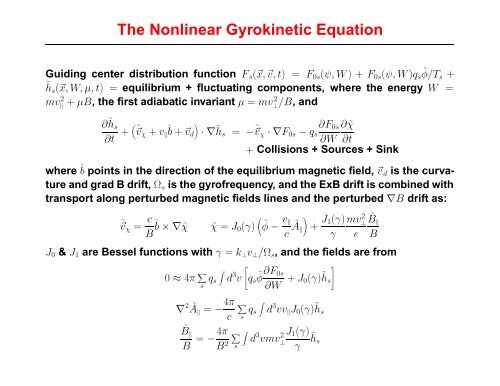
The Nonlinear Gyrokinetic Equation
Guiding center distribution function Fs(x, v, t) = F0s(ψ, W ) + F0s(ψ, W )qs ˜ φ/Ts +
˜hs(x, W, µ, t) = equilibrium + fluctuating components, where the energy W =
mv 2 + µB, the first adiabatic invariant µ = mv 2 ⊥/B, and
∂ ˜ hs
∂t
∂ ˜χ
∂W ∂t
+ Collisions + Sources + Sink
+ ˜vχ + v ˆ
b + vd · ∇˜ hs = −˜ ∂F0s
vχ · ∇F0s − qs
where ˆ b points in the direction of the equilibrium magnetic field, v d is the curvature
and grad B drift, Ωs is the gyrofrequency, and the ExB drift is combined with
transport along perturbed magnetic fields lines and the perturbed ∇B drift as:
˜vχ = c
B ˆ
b × ∇ ˜χ ˜χ = J0(γ) ˜φ − v c Ã
+ J1(γ) mv
γ
2 ⊥
e
J0 & J1 are Bessel functions with γ = k ⊥v⊥/Ωs, and the fields are from
0 ≈ 4π
s qs
d 3 v
∇ 2 Ã = − 4π
c
˜B 4π
= −
B B2
s
⎡
⎣qs ˜ φ ∂F0s
s qs
∂W + J0(γ) ˜ hs
d 3 vv J0(γ) ˜ hs
d 3 vmv 2 ⊥
J1(γ)
γ ˜ hs
⎤
⎦
˜B
B