introduction to gyrokinetic and fluid simulations of ... - Our Home Page
introduction to gyrokinetic and fluid simulations of ... - Our Home Page
introduction to gyrokinetic and fluid simulations of ... - Our Home Page

You also want an ePaper? Increase the reach of your titles
YUMPU automatically turns print PDFs into web optimized ePapers that Google loves.
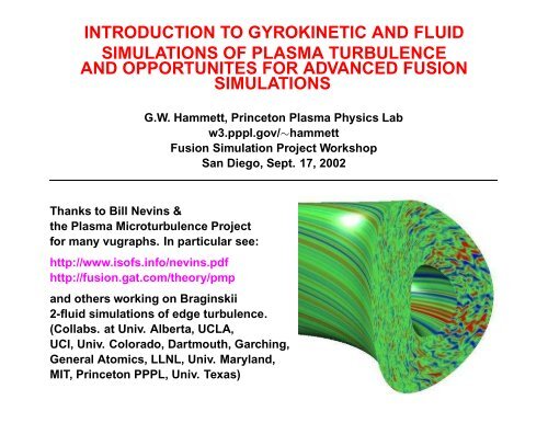
INTRODUCTION TO GYROKINETIC AND FLUID<br />
SIMULATIONS OF PLASMA TURBULENCE<br />
AND OPPORTUNITES FOR ADVANCED FUSION<br />
SIMULATIONS<br />
G.W. Hammett, Prince<strong>to</strong>n Plasma Physics Lab<br />
w3.pppl.gov/∼hammett<br />
Fusion Simulation Project Workshop<br />
San Diego, Sept. 17, 2002<br />
Thanks <strong>to</strong> Bill Nevins &<br />
the Plasma Microturbulence Project<br />
for many vugraphs. In particular see:<br />
http://www.is<strong>of</strong>s.info/nevins.pdf<br />
http://fusion.gat.com/theory/pmp<br />
<strong>and</strong> others working on Braginskii<br />
2-<strong>fluid</strong> <strong>simulations</strong> <strong>of</strong> edge turbulence.<br />
(Collabs. at Univ. Alberta, UCLA,<br />
UCI, Univ. Colorado, Dartmouth, Garching,<br />
General A<strong>to</strong>mics, LLNL, Univ. Maryl<strong>and</strong>,<br />
MIT, Prince<strong>to</strong>n PPPL, Univ. Texas)
A complete description <strong>of</strong> a plasma<br />
is given by the particle distribution function Fs(x, v, t), the density <strong>of</strong> particles<br />
at (near) position x with velocity v <strong>and</strong> time t, for species s (with charge q s <strong>and</strong><br />
mass ms).<br />
The charge density <strong>and</strong> current needed for Maxwell’s equations <strong>to</strong> determine<br />
the electric <strong>and</strong> magnetic fields is then:<br />
σ(x, t) = <br />
s qs<br />
<br />
d 3 vFs(x, v, t)<br />
Fs is determined by the Vlasov-Boltzmann equation<br />
∂F<br />
∂t<br />
+ v · ∂F<br />
∂x<br />
+ qs<br />
ms<br />
⎛<br />
⎞<br />
⎜<br />
⎝ E + v × B ⎟<br />
⎠ ·<br />
c<br />
∂F<br />
∂v<br />
j(x, t) = <br />
s qs<br />
<br />
d 3 vvFs(x, v, t)<br />
= Collisions + sources + sinks ≈ 0<br />
where sources + sinks includes radiation cooling <strong>of</strong> electrons, ionization <strong>and</strong><br />
recombination changes <strong>of</strong> ion charge state, etc.
Equivalent particle approach<br />
Discrete particle density representation (combined with smoothing <strong>and</strong><br />
“particle-in-cell” techniques):<br />
dxi<br />
dt<br />
= vi<br />
Fs = <br />
i=1,N<br />
wi(t)δ(x − xi(t)δ(v − vi(t)<br />
dvi<br />
dt<br />
= qi<br />
mi<br />
⎛<br />
⎜<br />
⎝ E(xi, t) + vi × B(xi, t)<br />
c<br />
plus Monte Carlo treatment <strong>of</strong> collisions, sources <strong>and</strong> sinks.<br />
Both “continuum” F <strong>and</strong> particle descriptions are equivalent (in the limit <strong>of</strong><br />
a large number <strong>of</strong> particles, typical fusion particle density ∼ 10 14 /cm 3 ) <strong>and</strong><br />
are“Exact”, but both include an excessive range <strong>of</strong> time <strong>and</strong> space scales.<br />
Most plasma phenomena <strong>of</strong> interest are slow compared <strong>to</strong> the electron <strong>and</strong> ion<br />
gyr<strong>of</strong>requencies (∼ 10 11 Hz <strong>and</strong> ∼ 10 8 Hz).<br />
⎞<br />
⎟<br />
⎠
The Nonlinear Gyrokinetic Equation<br />
Guiding center distribution function Fs(x, v, t) = F0s(ψ, W ) + F0s(ψ, W )qs ˜ φ/Ts +<br />
˜hs(x, W, µ, t) = equilibrium + fluctuating components, where the energy W =<br />
mv 2 + µB, the first adiabatic invariant µ = mv 2 ⊥/B, <strong>and</strong><br />
∂ ˜ hs<br />
∂t<br />
∂ ˜χ<br />
∂W ∂t<br />
+ Collisions + Sources + Sink<br />
<br />
<br />
+ ˜vχ + v ˆ<br />
b + vd · ∇˜ hs = −˜ ∂F0s<br />
vχ · ∇F0s − qs<br />
where ˆ b points in the direction <strong>of</strong> the equilibrium magnetic field, v d is the curvature<br />
<strong>and</strong> grad B drift, Ωs is the gyr<strong>of</strong>requency, <strong>and</strong> the ExB drift is combined with<br />
transport along perturbed magnetic fields lines <strong>and</strong> the perturbed ∇B drift as:<br />
˜vχ = c<br />
B ˆ <br />
b × ∇ ˜χ ˜χ = J0(γ) ˜φ − v c à <br />
<br />
+ J1(γ) mv<br />
γ<br />
2 ⊥<br />
e<br />
J0 & J1 are Bessel functions with γ = k ⊥v⊥/Ωs, <strong>and</strong> the fields are from<br />
0 ≈ 4π <br />
s qs<br />
<br />
d 3 v<br />
∇ 2 Ã = − 4π <br />
c<br />
˜B 4π<br />
= −<br />
B B2 <br />
<br />
s<br />
⎡<br />
⎣qs ˜ φ ∂F0s<br />
s qs<br />
<br />
∂W + J0(γ) ˜ hs<br />
d 3 vv J0(γ) ˜ hs<br />
d 3 vmv 2 ⊥<br />
J1(γ)<br />
γ ˜ hs<br />
⎤<br />
⎦<br />
˜B <br />
B
˜E = −∇ ˜ φ − 1 ∂<br />
c<br />
à ∂t ˆb B = B0 + ∇ Ã × ˆ b + ˜ B ˆ b<br />
In a full-<strong>to</strong>rus simulation where plasma variations must be kept<br />
J0(k ⊥v ⊥/Ωs)φ → 〈φ〉(x) = 1<br />
2π<br />
<br />
dρφ(x + ρ)
C<strong>and</strong>y/Waltz movies available at:<br />
http://web.gat.com/comp/parallel/gyro gallery.html<br />
<strong>and</strong> other movies can be found from various links starting at:<br />
http://fusion.gat.com/theory/pmp
The Plasma Microturbulence<br />
Project supports a 2x2 matrix<br />
<strong>of</strong> codes (geometry x algorithm),<br />
each type <strong>of</strong> code is tuned <strong>to</strong><br />
optimize in various regimes <strong>and</strong><br />
so are optimized <strong>to</strong> study certain<br />
types <strong>of</strong> problems.<br />
Codes using flux-tube geometry<br />
(shown here) take advantage <strong>of</strong><br />
short decorrelation lengths <strong>of</strong> the<br />
turbulence perpendicular <strong>to</strong> magnetic<br />
field lines. Multiple copies <strong>of</strong><br />
a flux-tube pasted <strong>to</strong>gether represent<br />
a <strong>to</strong>roidal annulus.
We Support a 2x2 Matrix <strong>of</strong><br />
Plasma Turbulence Simulation Codes<br />
Continuum PIC<br />
Flux Tube GS2 SUMMIT<br />
Global GYRO GTC<br />
• Why both Continuum <strong>and</strong> Particle-in-Cell (PIC)?<br />
– Cross-check on algorithms<br />
– Continuum currently most developed (already has kinetic e’s , B )<br />
– PIC may ultimately be more efficient<br />
• If we can do Global <strong>simulations</strong>, why bother with Flux Tubes?<br />
– Electron-scale ( e , e =c/ pe ) physics (ETG modes, etc.)<br />
– Turbulence on multiple space scales (ITG+TEM, TEM+ETG, ITG+TEM+ETG, …)<br />
– Efficient parameter scans<br />
June 5, 2002 Plasma Microturbulence Project 3
Current ‘state-<strong>of</strong>-the-art’<br />
(similar performance achieved in Continuum codes)<br />
Spatial Resolution<br />
• Plasma turbulence is quasi-2-D<br />
Temporal Resolution<br />
• Studies <strong>of</strong> turbulent fluctuations<br />
– Resolution requirement along B–field<br />
determined by equilibrium structure<br />
– Resolution across B–field determined<br />
by microstructure <strong>of</strong> the turbulence.<br />
⇒ ~ 64×(a/ρi ) 2 ~ 2×10⁸ grid points <strong>to</strong><br />
simulate ion-scale turbulence at<br />
burning-plasma scale in a global code<br />
– Require ~ 8 particles / spatial grid point<br />
⇒ ~ 1.6×10⁹ – Characteristic turbulence time-scale<br />
–<br />
⇒ cs /a ~ 1 µs (10 time steps)<br />
Correlation time >> oscillation period<br />
⇒ τc ~ 100× cs /a ~ 100 µs<br />
(10<br />
particles for global ionturbulence<br />
simulation at ignition scale<br />
– ~ 600 bytes/particle<br />
⇒ 1 terabyte <strong>of</strong> RAM<br />
⇒ This resolution is achievable<br />
3 –<br />
time steps)<br />
Many τc ’s required<br />
⇒ Tsimulation ~ few ms<br />
(5×10⁴ time steps)<br />
– 4×10⁻⁹ sec/particle-timestep<br />
(this has been achieved)<br />
⇒ ~90 hours <strong>of</strong> IBM-SP time/run<br />
* Heroic (but within our time allocation)<br />
(Such <strong>simulations</strong> have been performed, see T.S. Hahm, Z. Lin, APS/DPP 2001)<br />
• Simulations including electrons <strong>and</strong> B (short space & time scales) are not<br />
yet practical at the burning-plasma scale with a global code<br />
5/23/02 W.M. Nevins, "Turbulence & Transport" 7
Major Computational <strong>and</strong><br />
Applied Mathematical Challenges<br />
• Continuum kernels solve an advection/diffusion equation on a 5-D grid<br />
– Linear algebra <strong>and</strong> sparse matrix solves (LAPAC, UMFPAC, BLAS)<br />
– Distributed array redistribution algorithms (we have developed or own)<br />
• Particle-in-Cell kernels advance particles in a 5-D phase space<br />
– Efficient “gather/scatter” algorithms which avoid cache conflicts <strong>and</strong> provide<br />
r<strong>and</strong>om access <strong>to</strong> field quantities on 3-D grid<br />
• Continuum <strong>and</strong> Particle-in-Cell kernels perform elliptic solves on 3-D grids<br />
(<strong>of</strong>ten mixing Fourier techniques with direct numerical solves)<br />
• Other Issues:<br />
– Portability between computational platforms<br />
– Characterizing <strong>and</strong> improving computational efficiency<br />
– Distributed code development<br />
– Exp<strong>and</strong>ing our user base<br />
5/23/02 W.M. Nevins, "Turbulence & Transport" 19
Continuum / Eulerian Codes Particle-in-Cell/Lagrangian Codes<br />
Flux-tube / thinannulus<br />
Full-<strong>to</strong>rus or thin annulus Flux-tube Full-<strong>to</strong>rus<br />
All now use field-line following coordinate systems, Δx⊥/Δx|| ~ ρi/L ~ 10 -1 -10 -3<br />
GS2 (Dorl<strong>and</strong>, U. Md.,<br />
Kotschenreuther)<br />
⊥ Pseudo-spectral<br />
linear & nonlinear.<br />
|| 2 cd order finite-diff.<br />
(slight upwind)<br />
Linear: fully implicit<br />
(elegant algorithm)<br />
Nonlinear: 2 cd order<br />
Adams-Bashforth<br />
Elliptic solvers easy<br />
in Fourier space<br />
Gyro (C<strong>and</strong>y-Waltz GA) Summit<br />
(LLNL, U. Co,<br />
UCLA)<br />
Toroidal pseudo-spectral<br />
5 th -6 th order upwind τ grid<br />
<strong>to</strong> avoid 1/v||<br />
collisions w/ direct sparse<br />
solver (UMFPACK)<br />
High accuracy explicit 4 th<br />
order Runge-Kutta<br />
GTC (Z. Lin et.al.<br />
PPPL, UCI)<br />
Delta-f algorithm reduces particle<br />
noise.<br />
Recent hybrid electron algorithm:<br />
<strong>fluid</strong> with kinetic electron closure.<br />
Leap-frog / Predic<strong>to</strong>r-correc<strong>to</strong>r<br />
Elliptic solvers with non-uniform coefficients solved by<br />
combination <strong>of</strong> Fourier, iterative, <strong>and</strong> direct matrix solution<br />
Fast time scales hiding in E & B fields: is there a partially-implicit iterative<br />
algorithm that can help?
Recommendations (I)<br />
Strengthening PMP Support <strong>to</strong> Integrated Modeling<br />
(1) Improve the fidelity <strong>and</strong> performance <strong>of</strong> Plasma<br />
Microturbulence Project codes<br />
(2) Validate these codes against experiment<br />
(3) Exp<strong>and</strong> the user base <strong>of</strong> the PMP codes<br />
(4) Initiate the development <strong>of</strong> a kinetic edge<br />
turbulence simulation code.<br />
5/23/02 W.M. Nevins, "Turbulence & Transport" 13
CORE TURBULENT TRANSPORT STILL IMPORTANT<br />
• Provides most <strong>of</strong> temperature gradient: 20 keV center → 1-4 keV near-edge.<br />
Effects <strong>of</strong> shaping, density peakedness, rotation, impurities, T i/Te?<br />
• Detailed experimental comparisons possible, fluctuation diagnostics.<br />
• Are internal transport barriers possible at reac<strong>to</strong>r scales? P threshold? Torque?<br />
Controllable?<br />
• Electron-scale transport controls advanced reac<strong>to</strong>r performance?<br />
BUT EDGE TURBULENCE CRITICAL<br />
• H-mode pedestal (edge transport barrier) greatest source <strong>of</strong> uncertainty for<br />
reac<strong>to</strong>r predictions.<br />
• Will diver<strong>to</strong>r melt/erode? Need ELM simulation.<br />
• Edge very complicated: Separatrix & diver<strong>to</strong>r geometry matters. Bootstrap<br />
current important, second stability regime. Half <strong>of</strong> power radiated, intense<br />
neutral recycling.<br />
• High <strong>and</strong> low collisionality regimes. Present edge codes are collisional <strong>fluid</strong>s,<br />
need kinetic extensions.
3-D Fluid Simulations <strong>of</strong><br />
Plasma Edge Turbulence<br />
BOUT (X.Q. Xu, )<br />
• Braginskii — collisional, two <strong>fluid</strong><br />
electromagnetic equations<br />
• Realistic ×-point geometry<br />
(open <strong>and</strong> closed flux surfaces)<br />
• BOUT is being applied <strong>to</strong> DIII-D,<br />
C-Mod, NSTX, …<br />
• There is LOTS <strong>of</strong> edge fluctuation data!<br />
⇒ An Excellent opportunity for<br />
code validation<br />
5/23/02 W.M. Nevins, "Turbulence & Transport" 15
More info:<br />
Plasma Microturbulence Project (PMP):<br />
http://fusion.gat.com/theory/pmp<br />
Nevins presentation on PMP <strong>to</strong> ISOFS May 2002:<br />
http://www.is<strong>of</strong>s.info/nevins.pdf<br />
GS2 (Dorl<strong>and</strong> Univ. Md.):<br />
http://gk.umd.edu/GS2/info.html<br />
Useful 2-page <strong>gyrokinetic</strong> summary:<br />
http://gk.umd.edu/GS2/gs2 back.ps<br />
GTC (Lin PPPL UCI):<br />
http://w3.pppl.gov/∼zlin/visualization/<br />
Gyro (C<strong>and</strong>y/Waltz GA):<br />
http://web.gat.com/comp/parallel/gyro.html<br />
Summit (LLNL/UCLA/U. Co.):<br />
http://www.nersc.gov/scidac/summit