Turbo Decoding and Detection for Wireless Applications

More documents

Recommendations

Info

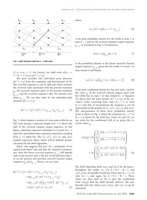
Fig. 3. MAP decoder trellis for K ¼ 3RSCcode. ðs0 ; sÞ )uk ¼ 1. For brevity, we shall write pðSk 1 ¼ s0 ^ Sk ¼ s ^ yÞ as pðs0 ^ s ^ yÞ. We now consider the individual joint densities pðs0 ^ s ^ yÞ from the numerator and denominator of (3). The received sequence y can be split into three sections: the received value associated with the present transition y , the received sequence prior to the present transition k y , and the received sequence after the present tran- j G k sition y . We can thus write for the individual joint j 9 k densities pðs0 ^ s ^ yÞ pðs 0 ^ s ^ yÞ ¼pðs 0 ^ s ^ y j G k ^ y k ^ y j 9 k Þ: (4) Fig. 3, which depicts a section of a four-state trellis for an RSC code having a constraint-length of K ¼ 3, shows this split of the received channel output sequence. In this figure, solid lines represent transitions as a result of a 1 input bit, and dashed lines represent transistion resulting from a þ1 input bit. The k 1ðs 0 Þ, kðs 0 ; sÞ, and kðsÞ symbols represent values, which will be defined shortly, calculated by the MAP algorithm. Bayes’ rule suggests that pða ^ bÞ ¼pðajbÞpðbÞ. Ifwe exploit both Bayes’ rule and that the channel is memoryless, then the future received sequence y j 9 k will depend only on the present state s, butnotonthepreviousstates 0 or on the present and previous received channel output sequences y k and y j G k . Hence, we can write pðs 0 ^ s ^ yÞ ¼pðs 0 ^ s ^ y j G k ^ y k ^ y j 9 k Þ ¼ pðy j 9 k jsÞ pðs 0 ^ s ^ y j G k ^ y k Þ ¼ pðy j 9 k jsÞ p fy k ^ sgjs 0 pðs 0 ^ y j G k Þ ¼ kðsÞ kðs 0 ; sÞ k 1ðs 0 Þ (5) Hanzo et al.: Turbo Decoding and Detection for Wireless Applications where k 1ðs 0 Þ¼pðSk 1 ¼ s 0 ^ y j G k Þ (6) is the joint probability density for the trellis at state s 0 at time k 1 and for the received channel output sequence y j G k ,asvisualizedinFig.3.Furthermore kðsÞ ¼pðy j 9 k jSk ¼ sÞ (7) is the probability density of the future received channel output sequence y j 9 k , given that the trellis is in state s at time instant k and finally kðs 0 ; sÞ ¼p fy k ^ Sk ¼ sgjSk 1 ¼ s 0 (8) is the joint conditional density for the next state s and for the value y k of the received channel output, given that the trellis was in state s 0 at time instant k 1. Equation (5) shows that the joint density pðs 0 ^ s ^ yÞ of the encoder’s trellis traversing from state Sk 1 ¼ s 0 to state Sk ¼ s and that of encountering the sequence y can be represented as the product of k 1ðs 0 Þ, kðs 0 ; sÞ, and kðsÞ. The interpretation of these three probability density terms is shown in Fig. 3, where the transition Sk 1 ¼ s 0 to Sk ¼ s is shown by the bold line. From (3) and (5), we can write for the conditional LLR of uk, given the received value y k P ðs LðukjyÞ¼ln 0 pðSk 1 ¼ s ;sÞ) uk¼þ1 0 ^ Sk ¼ s ^ yÞ P pðSk 1 ¼ s0 0 1 B C B C B C @ ^ Sk ¼ s ^ yÞA ðs 0 ;sÞ) u k ¼ 1 0 P B ¼ lnB P @ ðs0 ;sÞ) uk¼þ1 ðs 0 ;sÞ) u k ¼ 1 k 1ðs0Þ kðs0 ; sÞ kðsÞ k 1ðs0Þ kðs0 1 C C: (9) ; sÞ kðsÞA The MAP algorithm finds kðsÞ and kðsÞ for all states s throughout the trellis, i.e., for k ¼ 0; 1 N 1, and kðs 0 ; sÞ for all possible transitions from state Sk 1 ¼ s 0 to state Sk ¼ s, and again for k ¼ 0; 1 N 1. These values are then used in (9) to give the conditional LLRs LðukjyÞ that the MAP decoder delivers. We now describe how the values kðsÞ, kðsÞ, and kðs 0 ; sÞ can be calculated. Vol. 95, No. 6, June 2007 | Proceedings of the IEEE 1181
Hanzo et al.: Turbo Decoding and Detection for Wireless Applications 2) Forward Recursive Calculation of kðsÞ: Consider first kðsÞ. From the definition of k 1ðs 0 Þ in (6), we can write kðsÞ ¼pðSk ¼ s ^ y Þ j G kþ1 ¼ pðs ^ y ^ y Þ j G k k ¼ X pðs ^ s 0 ^ y ^ y Þ (10) j G k k all s 0 where in the last line we split the density pðs ^ y Þ y G kþ1 into the sum of joint densities pðs ^ s0 ^ y Þ over all j G kþ1 possible previous states s0 . Using Bayes’ rule and the assumption that the channel is memoryless again, we can proceed as follows: kðsÞ ¼ X all s0 pðs ^ s 0 ^ y ^ y Þ j G k k ¼ X all s0 p fs ^ y gjfs k 0 ^ y g pðs j G k 0 ^ y Þ j G k ¼ X all s0 p fs ^ y gjs k 0 pðs 0 ^ y Þ j G k ¼ X k 1ðs 0 Þ kðs 0 ; sÞ: (11) all s 0 Thus, once the kðs 0 ; sÞ values are known, the kðsÞ values can be calculated recursively. Assuming that the trellis has the initial state S0 ¼ 0, the initial conditions for this recursion are 0ðS0 ¼ 0Þ ¼1 0ðS0 ¼ sÞ ¼0 for all s 6¼ 0: (12) Fig. 4 shows an example of how one kðsÞ value, for s ¼ 0, is calculated recursively using values of k 1ðs 0 Þ and kðs 0 ; sÞ for our K ¼ 3 RSC code. Notice that, as we are considering a binary trellis, only two previous states, Sk¼1 ¼ 0 and Sk 1 ¼ 1, have paths to the state Sk ¼ 0. Therefore, the summation in (11) is over only two terms. 3) Backward Recursive Calculation of kðsÞ: Thevaluesof kðsÞ can similarly be calculated recursively. Using a similar derivation to that for (11), it can be shown that k 1ðs 0 Þ¼pðy j 9 k 1 js 0 Þ¼ X all s kðsÞ kðs 0 ; sÞ: (13) Thus, once the values kðs 0 ; sÞ are known, a backward recursion can be used to calculate the values of k 1ðs 0 Þ 1182 Proceedings of the IEEE |Vol.95,No.6,June2007 Fig. 4. Recursive calculation of kð0Þ and kð0Þ. from the values of kðsÞ using (13). Fig. 4 again shows an example of how the kð0Þ value is calculated recursively using values of kþ1ðsÞ and kþ1ð0; sÞ for our K ¼ 3 RSC code. 4) Calculation of kðs 0 ; sÞ: We now consider how the transition densities kðs 0 ; sÞ in (5) can be calculated from the received channel sequence and any aprioriinformation that is available. Using the definition of kðs 0 ; sÞ from (8) and the derivation from Bayes’ rule we have kðs 0 ; sÞ ¼p fy k ^ sgjs 0 ¼ p y k jfs 0 ^ sg Pðsjs 0 Þ ¼ p y k jfs 0 ^ sg PðukÞ ¼ pðy k jx k Þ PðukÞ (14) where uk is the input bit necessary to cause the transition from state Sk 1 ¼ s 0 to state Sk ¼ s, PðukÞ is the apriori probability of this bit, and x k is the transmitted codeword associated with this transition. Hence, the transition probability density kðs 0 ; sÞ is given by the product of the aprioriprobability of the input bit uk necessary for the transition and the conditional density of the received channel sequence for the value y k given that the codeword x k associated with the transition was transmitted. The a priori probability PðukÞ is derived in an iterative decoder from the output of the previous component decoder, andVassuming a memoryless additive white Gaussian noise (AWGN) channel and BPSK
Page 1 and 2: INVITED PAPER Turbo Decoding and De
Page 3: Hanzo et al.: Turbo Decoding and De
Page 7 and 8: Hanzo et al.: Turbo Decoding and De
Page 23: Hanzo et al.: Turbo Decoding and De

Turbo Decoding and Detection for Wireless Applications

Create successful ePaper yourself

Delete template?

Save as template?