770:313-36. Creating a hopeful monster: mouse - Emory University ...

Creating a “Hopeful Monster”: Mouse Forward
Genetic Screens
Vanessa L. Horner and Tamara Caspary
Abstract
Chapter 12
One of the most straightforward approaches to making novel biological discoveries is the forward genetic
screen. The time is ripe for forward genetic screens in the mouse since the mouse genome is sequenced,
but the function of many of the genes remains unknown. Today, with careful planning, such screens
are within the reach of even small individual labs. In this chapter we first discuss the types of screens in
existence, as well as how to design a screen to recover mutations that are relevant to the interests of a lab.
We then describe how to create mutations using the chemical N-ethyl-N-nitrosourea (ENU), including a
detailed injection protocol. Next, we outline breeding schemes to establish mutant lines for each type of
screen. Finally, we explain how to map mutations using recombination and how to ensure that a particular
mutation causes a phenotype. Our goal is to make forward genetics in the mouse accessible to any lab
with the desire to do it.
Key words: ENU, mutagenesis, mutant, phenotype-driven screen.
1. Introduction
Recent years have brought an explosion of whole-genome
sequencing in a wide variety of organisms. From this explosion,
comparative genomics has emerged as a powerful tool for shedding
light on a range of biological processes, with the potential
to reveal much about human variation, development, and disease.
However, comparative genomics will not fulfill its potential until
we have a more complete understanding of the functions of the
individual genes in these genomes, so they can be related back to
their human counterparts. For example, the function of a third
of the genes in the mouse genome is still completely unknown.
F.J. Pelegri (ed.), Vertebrate Embryogenesis, Methods in Molecular Biology 770,
DOI 10.1007/978-1-61779-210-6_12, © Springer Science+Business Media, LLC 2011
313

314 Horner and Caspary
Of the approximately 26,000 genes in the mouse genome, 8,154
(31%) genes have no functional annotation (1). Perhaps more
remarkably, 17,904 (68%) genes in the mouse genome have no
mutant alleles (1). Several international projects are underway
to produce null alleles of every gene in the mouse genome, so
that gene function can be inferred from the resulting phenotype
(2, 3). Such a “reverse genetics” approach will provide valuable
resources to the mouse community and fill many gaps in our
knowledge. Complementary to this approach is forward genetics,
which begins with a mutant phenotype in a biological process
of interest and then asks what gene is disrupted to produce that
particular phenotype. Forward genetic screens, therefore, can give
us an unbiased view of a biological process from which novel discoveries
can flow. Furthermore, the nature of the allele obtained
in a mutagenesis screen can tell us a great deal about a particular
protein’s role in a specific process in a way that deletion of
the protein cannot. Finally, another benefit of alleles created via
chemical mutagenesis is that they tend to mimic human disease
alleles (4).
Reverse genetics has become the preferred method for individual
labs studying specific mammalian genes. Recently, however,
a growing number of labs are interested in forward genetics,
largely for two reasons. First, the availability of the mouse genome
sequence has made positional cloning much more straightforward,
due in part to a denser set of markers that allows one to
more easily narrow down the region in which a mutation lies. Further,
we now know exactly how many genes are in any particular
region. This information, combined with available gene expression
data, makes it easier to prioritize which genes to sequence to
find the causative mutation. Second, mutagenesis screens in the
mouse have the unique ability to impartially reveal a collection
of genes involved in a biological process of interest. In the current
genomics era, where the focus is shifting from understanding
single gene products to understanding how networks of gene
products interact and influence one another, forward genetics is a
particularly apt and powerful tool.
How practical is it for an individual lab to perform a forward
genetic screen in the mouse? General concerns are time, breeding
space required, and cost. Although the time from mutagenization
to the establishment of mutant lines is about 1 year, much of
this is passive time spent waiting for males to recover fertility after
mutagenization and setting up crosses. The active screening time
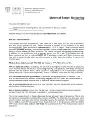
is 4 or 5 months. The amount of breeding space required reflects
this passive/active time pattern, with a long period of housing
relatively few mice, followed by the active screening phase, when
a burst of mice are produced (Fig. 12.1). Once mutant lines
are established, active positional cloning takes several months to
about a year to complete. However, next-generation resequencing
technology holds promise that we will further accelerate this

2. Materials
Creating a “Hopeful Monster”: Mouse Forward Genetic Screens 315
Fig. 12.1. Approximate breeding space required per month in a generic yearlong screen
for recessive mutations.
step, as longer portions of a chromosome can be sequenced for
less time and cost. Overall, it is quite feasible for an individual lab
to carry out a mutagenesis screen, and the goal of this chapter is to
provide the reader with practical considerations and instructions
to do just that.
1. Mice: 7- to 8-week-old males of the desired strain for mutagenization
(Section 3.2).
2. N-ethyl-N-nitrosourea (ENU).
3. 95% ethanol: make fresh each time.
4. Phosphate/citrate buffer: 0.1 M dibasic sodium phosphate
and 0.05 M sodium citrate, adjust to pH 5.0 with phosphoric
acid. Make fresh each time.
5. ENU inactivating solution: Use one of the following:
0.1 M potassium hydroxide
Alkaline sodium thiosulfate: 0.1 M sodium hydroxide and
1.3 M sodium thiosulfate.
6. Syringes/needles: For ENU dilution: 18-gauge needles,
10 mL syringes, and 30–50 mL syringes. For ENU injections:
25-gauge needles and 1 mL syringes.
7. Squirt bottles.
8. Waste containers: hazardous waste plastic bags, container
for deactivated ENU, and sharps disposal box.
9. Personal protective equipment for handling ENU: disposable
gowns, masks, gloves.
10. Disposable bench paper to line hood during ENU
injections.

316 Horner and Caspary
3. Methods
3.1. Designing
a Screen
The initial consideration is a critical one: how to design a screen
to recover mutations that suit the interests and goals of the lab?
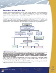
One way to approach this question is to first determine whether
you are interested in a general biological process or a particular
gene or region of the genome (Fig. 12.2). Those interested in
a general biological process are best served by a genome-wide
screen, since it is likely that numerous genes scattered throughout
the genome control the process of interest. Those more interested
in the functional content of a given region of the genome,
or in generating an allelic series of a particular gene, will find a
region-specific screen more appropriate. Another consideration is
the time it will take to map and clone causative mutations once
the screening is complete. In a genome-wide screen, the recovered
mutations can be at any position on any chromosome. Positional
cloning takes several months to a year to complete, because
one must generate enough embryos to allow up to 1,500 opportunities
for recombination, design primers to find polymorphic
markers, and sequence. Since region-specific screens are limited to
a defined portion of the genome, finding the causative mutation
is greatly simplified, reducing the overall time and cost. We will
examine several classes of both genome-wide and region-specific
genetic screens below.
Having defined screening criteria is another important factor
to consider when designing a screen, for ease of phenotype
identification and reproducibility. For example, our lab recently
completed a screen for recessive mutations that affect embryonic
development. We broadly examined embryos for morphological
abnormalities, but for consistency we chose nine key features to
Fig. 12.2. Classes of genome-wide and region-specific forward genetic screens.
Adapted with permission from Macmillan Publishers Ltd: Nat Rev Genet (33), copyright
2005.

3.1.1. Genome-Wide
Screens
Creating a “Hopeful Monster”: Mouse Forward Genetic Screens 317
score, such as brain lobes, eyes, and pharyngeal arches. Increasingly
complex assays can lead to lengthy or slow screening. For
instance, screens that include criteria such as serum analysis or
behavioral assays may limit the number of mutant lines that can
be screened. Each lab must weigh for itself the relative costs and
benefits of including extra steps in a screen.
Genome-wide screens can be designed to recover mutations that
create either dominant or recessive alleles. Dominant alleles cause
a phenotype that is observed in the heterozygous state, either
because two normal alleles are required for normal function of
the gene (haploinsufficiency), because the mutant allele disrupts
the function of the normal allele (dominant negative), or because
the mutant allele has new or increased activity (gain of function).
One purely practical reason to screen for dominant alleles is that
they can be recovered in the fewest number of crosses, thereby
reducing time and cost (Section 3.3). Another possible rationale
for performing a dominant screen is to model a human disease
condition with a dominant mode of transmission (for examples,
see (5)).
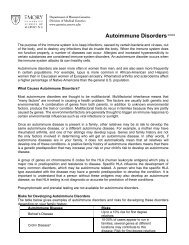
Recessive alleles can have partial or total loss of function, and
both alleles must be mutant to produce a phenotype. Therefore,
three crosses are required to recover mutations that create recessive
alleles (Fig. 12.3). The additional breeding time can be justified,
however, since it is easier to infer normal gene function from
recessive alleles, as they are generally loss of function.
The final class of genome-wide screen is the modifier screen:
recovering new genes that suppress or enhance a phenotype of
Fig. 12.3. Crossing scheme for dominant (upper gray box) or recessive (lower gray box)
mutant alleles. In this and all subsequent figures, chromosomes from the mutagenized
black mouse are represented as black bars; chromosomes from the white mouse are
represented as white bars. Additionally, in all figures stars represent mutant alleles.

318 Horner and Caspary
3.1.2. Region-Specific
Screens
interest. Modifier screens are performed when at least one gene
is known to be necessary for a biological process of interest, and
the goal is to discover other genes in the same pathway or same
process. Modifier screens can be designed to recover dominant or
recessive alleles, as above. They can also be performed with known
alleles that are not viable in the homozygous state, although the
crossing scheme is more involved (Fig. 12.4).
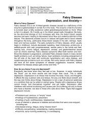
The narrowest type of region-specific screen is the noncomplementation
screen. The purpose of a non-complementation
screen is to find new alleles of a gene of interest, because
mutations in different protein domains can reveal much about
the function of those domains and/or can help to define specific
interactions with other proteins. In a non-complementation
screen, one crosses an animal carrying a known mutation in
a particular allele with an animal carrying random mutations
(Fig. 12.5). If the progeny of such a cross exhibit the mutant
phenotype of the known allele, the newly mutagenized allele is
said to “fail to complement” the original allele. It is important to
note that since mutations are induced randomly in the genome,
a failure to complement can be either allelic or non-allelic; if it is
allelic, then the mutation will be revealed through sequencing the
gene in the new mutant background. If it is non-allelic, the mutation
must be mapped via meiotic recombination (Section 3.4).
Deletion screens incorporate mouse strains with deletions in
known portions of their genome. A number of deletion strains are
available in the mouse, with about half of the chromosomes having
at least one “deletion complex” or collection of overlapping
deletions (Table 12.1). The first seven deletion complexes were
Fig. 12.4. Crossing scheme for dominant (upper gray box) or recessive (lower gray box)
modifier alleles. In this crossing scheme the allele to be modified (in the white mouse)
is assumed to be homozygous lethal or sterile. The half-black/half-white chromosome
in the second generation indicates that either allele is acceptable in this cross.

Creating a “Hopeful Monster”: Mouse Forward Genetic Screens 319
Fig. 12.5. Non-complementation crossing scheme. (a) The allele to be tested (in white
mouse) is viable and fertile as a homozygote. (b) The allele to be tested (in white mouse)
is lethal or sterile as a homozygote.
generated by irradiating or chemically mutating mice and then
crossing them to mice with visible markers. In this way deletions
could be located to the region surrounding the visible marker
(specific locus test; (6)). These initial deletion complexes each
contain many available mouse strains with overlapping deletions
(Table 12.1, gray rows). More recently, deletion complexes are
created in genomic areas of interest using embryonic stem cells
(ES cells). Deletions are generated in ES cells through irradiation
or through Cre–loxP-mediated recombination and then mice
bearing the deletions are produced from the ES cells, when possible
(Table 12.1, white rows) (7–10). In addition to simplifying
the mapping process, another practical reason to perform a deletion
screen is that recessive mutations can be recovered in fewer
crosses than in a genome-wide recessive screen (Fig. 12.6). The
only caveat is that the deletion strain used in the screen must be
viable as a heterozygote (i.e., cannot be haploinsufficient), a fact
not yet known for the deletions that only exist as ES cells.
The final region-specific screen is the balancer screen, modeled
after successful screens performed in Drosophila melanogaster
and Caenorhabditis elegans. A “balancer chromosome” is one that
contains inversions to prevent recombination with its homolog,
plus a dominant marker, so that animals carrying it can be recognized.
Balancer chromosomes may contain recessive lethal mutations
as well. They are called “balancers” because they prevent
any lethal or sterile mutations on the homologous chromosome
from being removed from a population (i.e., they maintain

320 Horner and Caspary
Table 12.1
Mouse chromosomal deletion complexes
Chr
Deletion
Complex
2 Non-agouti
(a)
No.
mouse/cell
lines Mode of generation
∼17 mouse
lines
Mixed (chemical
and radiation) of
mouse/germ cells
2 Notch1 10 cell lines ES cell:
recombinationmediated
deletion
4 Brown
(Tyrp1 b )
5 Hdh, Dpp6,
Gabrb1
∼35 mouse
lines
10 mouse
lines
7 Albino (Tyr c ) ∼55 mouse
lines
7 Pink-eyed
dilution (p)
9 Dilute
(Myo5a d )
9 Short ear
(Bmp5 se )
9 Dilute and
Short ear
(d se)
∼65 mouse
lines
∼16 mouse
lines
∼4 mouse
lines
∼29 mouse
lines
Mixed (chemical
and radiation) of
mouse/germ cells
ES cell: X-ray
irradiation
Mixed (chemical
and radiation) of
mouse/germ cells
Mixed (chemical
and radiation) of
whole mouse
Mixed (chemical
and radiation) of
mouse/germ cells
Mixed (chemical
and radiation) of
mouse/germ cells
Mixed (chemical
and radiation) of
mouse/germ cells
9 Ncam 28 cell lines ES cell: X and UV
irradiation
11 Hsd17b1 [Del
(11) Brd]
14 Piebald
(Ednrb s )
8 mouse lines ES cell:
recombinationmediated
deletion
20 mouse
lines
Mixed (chemical
and radiation) of
mouse/germ cells
15 Sox10 2 mouse lines ES cell: X-ray
irradiation
15 Oc90 2 mouse lines ES cell: X-ray
irradiation
15 Cpt1b 192 cell lines ES cell: X-ray
irradiation
Total span of
nested
deletions,
if known Reference
6.2–7.7 cM
(10.4 Mb)
(1, 6, 34, 35)
(36)
∼21 Mb (1, 6, 37–39)
40 cM (40)
6–11 cM for
29 of the
lines
28 cM (8)
8Mb (49)
(1, 6, 41, 42)
(1, 6, 43–45)
(1, 6, 46, 47)
(1, 6, 47, 48)
(1, 6, 47)
15.7–18 cM (1, 6, 50, 51)
577 kb (52)
658 kb-5 Mb (52)
(52)

Table 12.1
(continued)
Chr
Deletion
Complex
17 D17Aus9 3–7 mouse
lines
17 Sod2,
D17Leh94
Creating a “Hopeful Monster”: Mouse Forward Genetic Screens 321
No.
mouse/cell
lines Mode of generation
ES cell:
X-ray irradiation
8 mouse lines ES cell: X-ray
irradiation
X Hprt 4 cell lines ES cell:
recombinationmediated
deletion
X Hprt 9 cell lines ES cell: X and UV
irradiation
X Hprt 2 mouse lines ES cell: X-ray
irradiation
Total span of
nested
deletions, if
known Reference

322 Horner and Caspary
Fig. 12.7. Balancer screen crossing scheme. The white bar with double-sided arrows
indicates the balanced chromosome. In the first generation, F1 mice are crossed to
mice carrying the inversion in trans to a WT chromosome marked with a dominant
visible mutation (dotted bar with black circle). Mutant alleles are recovered in the third
generation (gray box).
rently there are not yet many balancer mouse strains available (see
Table 12.2). However, they can be generated using recombination
in ES cells (7, 11, 12). Furthermore, more G0 males may
need to be injected, because only half of the F1 males will be
subsequently used (those carrying the balancer, see Fig. 12.7).
Finally, when screening for embryonic lethal phenotypes, it is best
to use a balancer that is viable when homozygous to prevent confusion
about the cause of lethality.
3.2. Mutagenization There are several methods to mutagenize the mouse genome:
chemicals like N-ethyl-N-nitrosourea (ENU) and chlorambucil,
irradiation with X-rays or gamma rays, and transposons such
as sleeping beauty (6, 13–17). For the purposes of this chapter
we focus on the most widely used method, the chemical
ENU. ENU is a powerful mutagen. Depending on the strain of
mouse and the dose given, ENU induces a point mutation every
0.5–16 Mb throughout the genome (18–22), which is about 100
times higher than the spontaneous mutation rate per generation
in humans (23). Further, ENU primarily affects spermatogonial
stem cells, so that one male mouse will produce multiple clones
of mutated sperm after completion of spermatogenesis (24). In
addition to its efficient nature, another advantage of ENU is the
variety of protein altercations that can result from this form of
mutagenization. Since ENU is an alkylating agent that induces
point mutations, nonsense (10%), missense (63%), splicing (26%),
and “make-sense” (1%) mutations can all occur (reviewed in
(25–27)). Therefore, in addition to null alleles, other alleles
will also be generated, including hypomorphs, hypermorphs, and

Creating a “Hopeful Monster”: Mouse Forward Genetic Screens 323
Table 12.2
Mouse balancer strains (strains that are viable as homozygotes are indicated)
Chr Name
4 Inv
(4)Brd1 Mit281-Mit51
4 Inv
(4)Brd1 Mit117-Mit281
Dominant
marker
phenotype
(gene)
Coat color
(Tyrosinase and
K14-agouti)
Coat color
(Tyrosinase and
K14-agouti)
5 Rump white (Rw) Coat color (Kit
receptor tyrosine
kinase)
10 Steel panda (Sl pan ) Coat color (Kit
ligand)
11 Inv (11) Trp53-Wnt3 Coat color
(K14-agouti)
11 Inv (11) Wnt3-D11Mit69 Coat color
(K14-agouti)
11 Inv (11) Trp53-EgfR Coat color
(K14-agouti)
15 In (15)2R1 Short, hairy ears
(Eh)
15 In (15)21Rk Coat color
(K14-agouti)
3.2.1. Inbred Strains and
ENU Dose
Recessive
lethal?
(gene, if
known)
Mode of
generation Reference
No Cre–loxPmediated
recombination
No Cre–loxPmediated
recombination
(55)
(55)
Yes Irradiation (56, 57)
No Irradiation (58)
Yes (Wnt3) Cre–loxPmediated
recombination
Yes (Wnt3) Cre–loxPmediated
recombination
No Cre–loxPmediated
recombination
Yes Chemical
mutagenesis or
irradiation
Yes Modification of
line derived
from chemical
mutagenesis or
irradiation
(12)
(59)
(59)
(60)
(61)
dominant-negative alleles. This ability to generate an allelic series
is one of the great strengths of forward genetics.
One of the first practical considerations is which strain of mice to
mutagenize. A popular choice is C57BL/6J, because the effective
dose of ENU is well defined and the genome is sequenced for
this strain, facilitating future mapping and analysis portions of the
screen. Nevertheless, with the increased density of genetic markers
and cheaper and more advanced resequencing technologies,
choosing other strains has become feasible. Such advancements
allow more flexibility in screen design, for instance by enabling

324 Horner and Caspary
3.2.2. Number of Mice
to Inject
Table 12.3
Recommended dose of ENU for different inbred mouse strains
Inbred
mouse strain
Recommended
dose (mg/kg) a
No. days of
sterility
Percent
regained
fertility
A/J 3 × 90 74–113 90 (n = 10)
BALB/cJ 3 × 100 89–154 83 (n = 6)
BTBR/N 1 × 150–200 70–210 50–83 (ND)
C3He/J 3 × 85 96–148 70 (n = 10)
C3HeB/FeJ 3 × 75 89–142 90 (n = 10)
C57BL/6J 3 × 100 90–105 80 (n = 10)
a The doses are recommended based on the least amount of death and shortest period
of sterility. For details and alternate doses, see the original papers.
ND = no data.
Modified from (28, 29).
one to incorporate visible markers (such as GFP) that may only
be available on a particular genetic background. When choosing
the strain of mice to mutagenize, it is important to note that
ENU affects inbred strains differently (Table 12.3). In all strains,
ENU initially depletes all spermatogonia from the testes, leading
to a period of sterility from which some males never recover.
In addition, some mice may die during the sterile period due to
somatic mutations that lead to cancer or increase susceptibility
to pathogens. The length of the sterile period and the deaths
vary with ENU dosage and each inbred strain; some strains (like
BALB/cJ and C57BL/6J) can tolerate a relatively high dose,
whereas others (like FVB/N) are very sensitive to ENU. For successful
mutagenesis, one must balance the highest possible mutation
load with the lowest rates of sterility and death. Thanks to
careful analysis and experimentation by Justice et al. (28) and
Weber et al. (29), the optimal ENU dose for various inbred strains
can be estimated; we provide a summary in Table 12.3. Asindicated
in Table 12.3, a fractionated series of injections at weekly
intervals is generally more effective than one single large injection,
since a series maximizes the mutagenic effect and minimizes
animal lethality (30). For instance, rather than a single dose of
300 mg/kg, inject 3 doses of 100 mg/kg at weekly intervals
(written as 3 × 100 mg/kg).
The number of males to inject depends on how many genes in
the genome one wishes to survey. Each F1 animal is estimated
to be heterozygous for about 20–30 gene-inactivating mutations,
based on the specific locus test and data from other mutagenesis
screens (6, 31). In a genome-wide screen, 100 F1 lines will

3.2.3. ENU Injection
Protocol
3.2.3.1. Prior to Injection
3.2.3.2. Day of Injection
Creating a “Hopeful Monster”: Mouse Forward Genetic Screens 325
therefore interrogate 2,000–3,000 genes, about 8–12% of the
genome. Since ENU mutagenizes spermatogonial stem cells leading
to clones of mutant sperm, not more than eight F1 animals
should come from any particular G0 father, to avoid rescreening
the same mutation. In theory, for 100 F1 lines, a minimum of
12–13 G0 males should be injected. However, since some percentage
of the G0 males will either fail to recover fertility or die
(or both), it is good practice to inject about three times the minimum
number of males. For example, in a recently completed
genetic screen in our lab, we injected 50 C57/BL6 males with 3
× 100 mg/kg ENU. After 10–12 weeks, about half the males had
died before recovering fertility. From the remaining G0 males, we
recovered 122 F1 males.
ENU is carcinogenic and must be handled with extreme care
(modified from (32)). Most institutions require an IACUC safety
approval justification and common FAQs on ENU. ENU can be
obtained as 1 g of powder in a light-protected ISOPAC container.
ENU is sensitive to light, humidity, and pH. For this reason, it
should be stored at –20 ◦ C in the dark until use and then diluted
not more than 3 h before injection.
1. Complete all institutional IACUC safety approval procedures
(varies from institution to institution).
2. Order male mice of the strain to be injected so that they will
be 7–8 weeks old at the time of injection, keeping in mind
that they will need at least 1 week to adjust to their new
environment after arrival.
3. Make all solutions and gather all materials (see above).
4. Weigh all males to be injected and calculate the amount of
ENU to inject per mouse, based on the following formula:
10 mg/mL ENU (x mL to inject)
= (final concentration of ENU)(mouse body weight)
For example, if you want a final concentration of 100 mg/kg
ENU in a 20 g C57BL/6J mouse:
10 mg/mL ENU (x mL to inject) = (0.1 mg/g)(20 g)
x = 0.2 mL of 10 mg/mL ENU, for a final concentration of
100 mg/kg ENU
5. Dissolve and dilute ENU to 10 mg/mL (see Note 1):
a. Inject 10 mL of 95% ethanol into the ISPOAC container.
Swirl gently to dissolve. When dissolved, ENU is a clear
yellow liquid.

326 Horner and Caspary
3.2.3.3. After Injection
3.3. Breeding
Crosses and
Establishment
of Mutant Lines
3.3.1. Genome-Wide
Screen: Dominant
Mutations
b. Vent ISOPAC with an 18-gauge needle. Inject 90 mL of
phosphate/citrate buffer into container.
6. Inject mice: an experienced person familiar with intraperitoneal
injections should inject each mouse with the proper
volume (determined from the formula above) following
standard procedures.
7. After injection, the mice will become uncoordinated from
the alcohol and lose consciousness for a short time, usually
about 20 min. During this time they should be monitored
to ensure they recover consciousness.
8. Deactivate and dispose of ENU: ENU should be completely
deactivated. Since it has a short half-life under alkaline conditions,
use one of the two inactivating solutions given above
to thoroughly rinse all materials that came in contact with
ENU. In our experience it is best to minimize handling
the materials on the day of injection; therefore, we leave all
materials in the hood with the light on overnight to further
ensure that the ENU is deactivated. Prominent signs should
be displayed on the hood and room in which ENU is deactivating,
alerting unknowing staff and coworkers to the presence
of ENU.
9. After the last weekly injection, let males recover for 2–3
weeks.
10. A good indication that the mutagenesis was successful is
sterile males. To ensure that males are sterile, mate them
with females (at this time the females can be any strain
and can likely be used for other experiments if the males
are indeed sterile). Males are sterile if mating plugs are
observed but the females do not become pregnant.
11. Starting 2–3 weeks before the males are expected to regain
fertility (see Table 12.3), set males up with 1 or 2 females
of the desired strain (usually different from the G0 strain,
for mapping purposes, see below).
Once the G0 males have recovered fertility, the more active phase
of the screening process begins: breeding crosses to screen for
mutant phenotypes and establish mutant lines. The class of screen
dictates the series of crosses to perform; each crossing scheme is
outlined below.
1. 1st cross: Cross the mutagenized G0 male to one or two
females of a different (preferably inbred) strain. It is advantageous
to cross the G0 males to females of a different
strain, as polymorphic markers between the strains permit

Creating a “Hopeful Monster”: Mouse Forward Genetic Screens 327
Table 12.4
The number of informative SNPs between common inbred strains. The polymorphic
SNPs are derived from a low-density whole-genome SNP panel of 768 SNPs
C57BL/
6J
129X1/
SvJ
BALB/
cJ
C3H/
HeJ
DBA/2J FVB/NJ A/J CBA/J C57BL/
10J
C57BL/6J 508 497 598 555 539 581 562 68
129X1/SvJ 315 333 365 316 367 313 455
BALB/cJ 233 323 285 203 262 448
C3H/HeJ 241 294 226 111 552
DBA/2J 323 325 235 518
FVB/NJ 274 281 492
A/J 276 547
CBA/J 514
From the Mutation Mapping and Developmental Analysis Project (MMDAP), with permission from J. L. Moran and
D. R. Beier (personal communication).
3.3.2. Genome-Wide
Screen: Recessive
Mutations
straightforward mutation mapping (Section 3.4). The number
of polymorphisms between strains varies, so this should
be taken into account when choosing the crossing strain
(Table 12.4).
2. Dominant mutations will be recovered in the first generation
(F1) (upper gray box in Fig. 12.3). Since the mutations
occur randomly in the sperm of the G0 male, each F1 animal
represents a unique suite of mutations and is thus considered
a “line.” However, since the G0 spermatogonial stem cells
are mutated, it is best to screen not more than eight F1 animals
from any one G0 male to avoid rescreening the same
mutation. Collect F1 animals and screen for the phenotype
of interest. Once F1 animals with an interesting phenotype
are identified, they must be maintained as separate lines. If
the dominant mutation is viable and fertile, it is simply a
matter of breeding the F1 animal to the same inbred strain
chosen in cross #1.
1. 1st cross: Same as above. Collect eight F1 males per G0 male
and allow them to come to breeding age. Discard F1 females
(Fig. 12.3).

328 Horner and Caspary
3.3.3. Genome-Wide
Screen: Dominant or
Recessive Modifier
3.3.4. Region-Specific
Screen:
Non-complementation,
if the Starting Allele Is
Homozygous Viable and
Fertile
2. 2nd cross: Breed each F1 male individually to two wild-type
females of the same inbred strain used in the 1st cross.
Collect G2 females only and allow them to come to breeding
age; discard G2 males to save mouse room space and cost
(new G2 males can be obtained later, if needed, to establish
lines of interest).
3. 3rd cross: Backcross G2 females to their F1 fathers. Mate at
least six G2 females to each F1 male. When a phenotype has
been observed in at least two G3 animals from two separate
G2 females, it is likely genetic (see Note 2). To maintain
the line, collect G2 males and mate them to their sibling G2
females to determine whether the G2 male is a carrier; carrier
males are then kept for subsequent breeding and analysis
(Section 3.4).
Alternative 3rd cross: A theoretical drawback to backcrossing the
G2 females to F1 males is that it places reproductive strain on
the F1 male, since he will be needed to produce many litters.
In our experience, however, we have not encountered problems
with this. Nonetheless, an alternative to backcrossing is intercrossing
G2 male and female siblings. This method has the advantage
that G2 carrier males are immediately identified; a drawback is
that both G2 males and females must be weaned from the second
cross, above, increasing mouse room space and cost.
The breeding scheme presented here assumes that the mutation
to be modified is not viable in the homozygous state (white
mouse in Fig. 12.4).
1. 1st cross: Cross G0 males to females of a different strain who
are heterozygous for the allele to be modified. Collect F1
animals (not more than eight per G0 male, as above) and
allow them to come to breeding age.
2. 2nd cross: Cross F1 animals to animals of the same strain as
the females crossed to G0 males, above. Dominant modifiers
will be seen in G2 animals; collect and screen for enhancement
or suppression of the phenotype of interest.
3. 3rd cross: Backcross G2 females to their F1 fathers. Recessive
modifiers will be seen in G3 animals; collect and screen for
enhancement or suppression of the phenotype of interest.
1. 1st cross: Cross G0 males with females of a different inbred
strain who are homozygous for the allele of interest. Collect
F1 animals (not more than eight per G0 male, as
above) and screen them for failure to complement the mutation
(Fig. 12.5) (i.e., exhibit the same phenotype as animals
homozygous for the starting allele (white mouse in
Fig. 12.5a)).

3.3.5. Region-Specific
Screen:
Non-complementation, if
the Starting Allele Is
Homozygous Lethal or
Sterile
3.3.6. Region-Specific
Screen: Deletion Screen
for Lethal or Sterile
Recessive Mutations
3.3.7. Region-Specific
Screen: Using Balancers
3.4. Analysis and
Cloning
Creating a “Hopeful Monster”: Mouse Forward Genetic Screens 329
1. 1st cross: Cross G0 males with wild-type females of the same
genetic background as those containing the allele of interest.
Collect F1 animals (not more than eight per G0 male, as
above) and allow them to come to breeding age.
2. 2nd cross: Cross F1 animals to animals that are heterozygous
for the allele of interest. Screen the resulting G2 progeny for
a failure to complement the allele of interest. As mentioned
above, a failure to complement (Fig. 12.5) can be either
allelic or non-allelic, and this can be determined through
direct sequencing of the gene in the new mutant background
(White Mouse in Fig. 12.5b).
1. 1st cross: Cross G0 males to wild-type females from the same
genetic background as the deletion strain used in the 2nd
cross, below. Collect F1 animals and allow them to come to
breeding age (Fig. 12.6).
2. 2nd cross: Cross F1 animals to animals hemizygous for a
deleted region of interest. Any recessive mutations that
occur in trans to the deleted region will be observable in
the G2 progeny.
1. 1st cross: Cross G0 males to females of a different inbred
strain who are heterozygous for a balancer chromosome.
Collect F1 animals carrying the balancer chromosome (onehalf
of the F1 progeny) and allow them to come to breeding
age (Fig. 12.7).
2. 2nd cross: Cross F1 animals carrying the balancer to animals
carrying the balancer in trans to a wild-type chromosome
marked with a dominant visible marker that is distinct
from the visible marker on the balancer chromosome. Collect
G2 animals that are heterozygous for the newly mutated
chromosome over the balancer chromosome (can be distinguished
based on visible markers). Discard the rest of the
progeny.
3. 3rd cross: Backcross G2 animals to their F1 parents. The G3
animals can again be distinguished by their visible markers. If
a G3 animal is not carrying a balancer chromosome, then it
is homozygous for the newly mutated chromosome. If such
animals exhibit a phenotype, then the mutation lies in the
balanced region of the genome. However, if a G3 animal
has a phenotype but is heterozygous for the balancer, then
the mutation lies outside the balanced region, elsewhere in
the genome.
The excitement of establishing a new mutant line with an interesting
phenotype may only be surpassed by discovering the

330 Horner and Caspary
3.4.1. Mapping Based
on Recombination
underlying genetic change that causes the phenotype. Traditionally,
there are three main steps to accomplish this goal: recombination
mapping to narrow down the genomic interval in which a
mutation lies, sequencing candidate genes in this genomic interval,
and confirming that a particular mutation is indeed responsible
for the observed phenotype.
Since mice from one inbred strain (x) are mutagenized and then
crossed to mice of another inbred strain (y), the F1 generation
is 50% x and 50% y. In the process of establishing and maintaining
mutant lines, mice are continually crossed to the nonmutagenized
(y) background, all the while selecting for the mutation.
Over several generations, therefore, the genome of the
mutant lines will largely be of the y background, while the region
surrounding the mutation will be of the x background. The
premise of recombination mapping is that the causative mutation
will be linked to the x background, which can be distinguished
by polymorphisms that differ between the x and y backgrounds.
There are two main classes of polymorphisms used in
recombination mapping: simple sequence length polymorphisms
(SSLPs), which are short repeated segments that differ in length
between inbred strains, and single nucleotide polymorphisms
(SNPs). Both classes can be used to create polymorphic “markers.”
SSLP markers are created by designing PCR primers around
the SSLP, so that the size of the PCR product differs between
two strains. SNP markers can be created by finding SNPs that
create restriction fragment length polymorphisms (RFLPs), also
detectable by PCR. In addition, SNPs can be genotyped directly
using array-based SNP panels (see below).
The first step of recombination mapping is to determine on
which chromosome the mutation lies. This is achieved by performing
a genome-wide scan using polymorphic markers that are
spaced at regular intervals throughout the genome at low density.
Several commercially available SNP panels have been designed
for this purpose. For example, Illumina’s mouse Low Density
(LD) and Medium Density (MD) Linkage Panels contain 377 and
1,449 SNPs, respectively, spaced across the entire mouse genome.
DNA from affected (mutant) animals is obtained, and the SNPs
contained in the linkage panels are genotyped to determine which
chromosome has the largest cluster of DNA from the mutagenized
background. The required starting amount of DNA is low
(750 ng–1.5 μg) and can be obtained from tissue from a single
animal. To detect linkage, DNA from eight or nine affected animals
should be SNP genotyped.
The next step is high-resolution mapping, which is essentially
the same process, but using markers that are more closely spaced.
In the course of mapping their own mutations, several groups
have created polymorphic markers and made them available to

Creating a “Hopeful Monster”: Mouse Forward Genetic Screens 331
the public (see online resources, below). You should first determine
whether any of the available markers are appropriate for your
use. If there are no informative markers in the region of interest,
then markers will need to be created. Step-by-step instructions
are available from the Sloan-Kettering site, below. Use the markers
to genotype both affected and non-affected animals from each
line. Since affected animals are known to carry the mutation, and
the mutation lies in a region of mutagenized background DNA
(e.g., “x”), informative animals will be recombinants that have
wild-type DNA (e.g., y) adjacent to mutagenized DNA. Since the
portion of the chromosome containing wild-type DNA cannot
contain the mutation, that portion can be ruled out. As more
affected recombinant animals are genotyped, longer portions of
the chromosome are eliminated. Conversely, non-affected recombinant
animals are used to rule out portions of the chromosome
that are homozygous for mutagenized DNA (for recessive alleles).
It is important to note that, if there are any issues with penetrance
of the phenotype one can easily be misled by apparently
non-affected animals and may want to exclude them from analysis.
Below is a partial list of online resources to locate or design
appropriate markers:
Sloan-Kettering Mouse Project Website: https://mouse.mskcc.
org
1. MarkerBase: Provides a list of available Sloan-Kettering
Institute (SKI) developed makers, a searchable database
of Massachusetts Institute of Technology (MIT) markers,
and a guide to create your own.
Mouse Genome Informatics (MGI): www.informatics.jax.org
1. Integrated Whitehead/MIT Linkage and Physical maps:
Provides a list of available MIT markers by chromosome:
www.informatics.jax.org/reports/mitmap
2. Strains, SNPs, and polymorphisms
a.SNP query: search for SNPs by strain, SNP attributes,
genomic position, or associated genes.
b.Search for RFLP- or PCR-based polymorphisms by
strain, locus symbol, or map position.
Ensembl Genome Browser: www.ensembl.org/Mus_
musculus/Info/Index
1. Browse for SNPs by chromosome (karyotype) or enter
genomic location.
a. Genetic variation: resequencing data for nine inbred
strains are compared with the C57BL/6J genomic
sequence, and SNPs are highlighted.
3.4.2. Sequencing Once the genomic interval in which a mutation lies has been narrowed
sufficiently, the next step is to sequence candidate gene(s)
in the interval. A number of factors influence the decision of when

332 Horner and Caspary
and what to begin sequencing. One consideration is whether
there are additional polymorphisms that could potentially narrow
the interval further. However, the chance of obtaining recombinant
animals decreases as the interval is narrowed. Perhaps the
best indicator that the time to sequence has come is that there are
a manageable number of genes in the interval, which may or may
not be correlated with the physical size of the interval. What is
“manageable” depends on the investigator, but larger collections
of genes can be prioritized for sequencing based on expression
data or any available phenotypic data. In addition, since ENU
causes mutations in exons and splice sites in the vast majority of
cases, sequencing entire genes is not necessary.
The availability of next-generation resequencing technologies
is poised to change how investigators perceive what is a manageable
number of genes to sequence. It is becoming practical to
sequence very long portions of a chromosome at a time and for
less money. This technology may drastically alter the balance of
time spent mapping versus sequencing, to the point that, ultimately,
one may only need to know which chromosome contains
the mutation before beginning to sequence.
3.4.3. Confirmation How do you know that a mutation actually causes the observed
phenotype? Direct evidence includes genetic rescue or complementation.
Genetic rescue occurs when a wild-type copy of the
gene is introduced into the mutant background, and the mutant
phenotype is no longer observed. Although direct, this method
is time consuming because it involves creating transgenic mice.
The other direct method is a complementation analysis, which
involves creating mice that have one copy of your mutant allele
and one copy of a known mutant allele in the suspected gene. If
the mutant phenotype is seen in such an animal, then your allele
fails to complement the phenotype and is an allele of the suspected
gene. While this is faster than genetic rescue, it depends
on the availability of mutant alleles in the gene of interest. There
can also be indirect evidence that a mutation causes the observed
phenotype, including disruption of gene expression, protein production,
protein activity, or cellular/tissue localization. Other
indirect evidence may be that the observed mutant phenotype
is similar to other alleles of the suspected gene or is similar to the
mutant phenotype of genes in the same pathway.
4. Notes
1. ENU: To spec or not to spec? The concentration of ENU
can be determined by spectrophotometry after dilution
in phosphate/citrate buffer. This is the best way to be

References
1. Bult, C. J., Eppig, J. T., Kadin, J. A., Richardson,
J. E., and Blake, J. A. (2008) The Mouse
Genome Database (MGD): mouse biology
and model systems. Nucleic Acids Res. 36,
D724–728.
2. Collins, F. S., Finnell, R. H., Rossant, J., and
Wurst, W. (2007) A new partner for the international
knockout mouse consortium. Cell
129, 235.
3. Collins, F. S., Rossant, J., Wurst, W., and
Consortium, T. I. M. K. (2007) A mouse for
all reasons. Cell 128, 9–13.
4. O‘Brien, T. P. and Frankel, W. N. (2004)
Moving forward with chemical mutagenesis
in the mouse. J. Physiol. 554, 13–21.
5. Hamosh, A., Scott, A. F., Amberger, J.
S., Bocchini, C. A., and McKusick, V. A.
(2005) Online Mendelian Inheritance in
Man (OMIM), a knowledgebase of human
genes and genetic disorders. Nucleic Acids
Res. 33, D514–517.
6. Russell, W. L., Kelly, E. M., Hunsicker, P. R.,
Bangham, J. W., Maddux, S. C., and Phipps,
E. L. (1979) Specific-locus test shows ethyl-
Creating a “Hopeful Monster”: Mouse Forward Genetic Screens 333
absolutely certain about the exact amount of ENU you are
injecting into the mice, since it is possible that there is not
exactly 1 g of ENU in the container provided by Sigma.
Problems can result if the amount of ENU injected is too
high (e.g., all the G0 males die or fail to recover fertility)
or too low (e.g., failure to obtain relevant mutant lines). If
you are experiencing one of these problems despite having
taken the inbred mouse strain into consideration, you may
need to spec the ENU. A good protocol can be found in
(32). However, in our experience we have found that handling
the ENU as little as possible is best, and following the
strain guidelines and injecting a sufficient number of males
yield good results.
2. It may be hard to tell if a particular phenotype is truly genetic
or just a random phenomenon. A good rule of thumb is that
the phenotype should be seen in multiple animals from separate
litters, at a frequency of approximately 25% (for recessive
alleles).
If screening for embryonic lethal mutations, the
G2 females will be dissected to view the G3 embryos. To
avoid an overwhelming number of dissections on any 1 day,
it is best to mate only two G2 females to the F1 male at
a time. As mating plugs are observed, place the pregnant
females in a separate cage and replenish the mating cage with
new G2 females.
nitrosourea to be the most potent mutagen
in the mouse. Proc. Natl. Acad. Sci. USA 76,
5818–5819.
7. Mills, A. A. and Bradley, A. (2001) From
mouse to man: generating megabase chromosome
rearrangements. Trends Genet. 17,
331–339.
8. Thomas, J. W., LaMantia, C., and Magnuson,
T. (1998) X-ray-induced mutations
in mouse embryonic stem cells. Proc. Natl.
Acad. Sci. USA 95, 1114–1119.
9. You, Y., Bergstrom, R., Klemm, M., Lederman,
B., Nelson, H., Ticknor, C., Jaenisch,
R., and Schimenti, J. (1997) Chromosomal
deletion complexes in mice by radiation
of embryonic stem cells. Nat. Genet. 15,
285–288.
10. You, Y., Browning, V. L., and Schimenti, J.
C. (1997) Generation of radiation-induced
deletion complexes in the mouse genome
using embryonic stem cells. Methods 13,
409–421.
11. Hentges, K. E. and Justice, M. J. (2004)
Checks and balancers: balancer chromosomes

334 Horner and Caspary
to facilitate genome annotation. Trends
Genet. 20, 252–259.
12. Zheng, B., Sage, M., Cai, W. W., Thompson,
D. M., Tavsanli, B. C., Cheah, Y.
C., and Bradley, A. (1999) Engineering a
mouse balancer chromosome. Nat. Genet.
22, 375–378.
13. Flaherty, L., Messer, A., Russell, L. B.,
and Rinchik, E. M. (1992) Chlorambucilinduced
mutations in mice recovered in
homozygotes. Proc. Natl. Acad. Sci. USA 89,
2859–2863.
14. Russell, L. B., Hunsicker, P. R., Cacheiro,
N. L., Bangham, J. W., Russell, W. L., and
Shelby, M. D. (1989) Chlorambucil effectively
induces deletion mutations in mouse
germ cells. Proc. Natl. Acad. Sci. USA 86,
3704–3708.
15. Russell, L. B. and Russell, W. L. (1992) Frequency
and nature of specific-locus mutations
induced in female mice by radiations
and chemicals: a review. Mutat. Res. 296,
107–127.
16. Russell, W. L. (1951) X-ray-induced mutations
in mice. Cold Spring Harb. Symp.
Quant. Biol. 16, 327–336.
17. Takeda, J., Keng, V. W., and Horie, K.
(2007) Germline mutagenesis mediated by
Sleeping Beauty transposon system in mice.
Genome Biol. 8 Suppl. 1, S14.
18. Beier, D. R. (2000) Sequence-based analysis
of mutagenized mice. Mamm. Genome 11,
594–597.
19. Chen, Y., Yee, D., Dains, K., Chatterjee, A.,
Cavalcoli, J., Schneider, E., Om, J., Woychik,
R. P., and Magnuson, T. (2000) Genotypebased
screen for ENU-induced mutations in
mouse embryonic stem cells. Nat. Genet. 24,
314–317.
20. Coghill, E. L., Hugill, A., Parkinson, N.,
Davison, C., Glenister, P., Clements, S.,
Hunter, J., Cox, R. D., and Brown, S. D.
(2002) A gene-driven approach to the identification
of ENU mutants in the mouse. Nat.
Genet. 30, 255–256.
21. Concepcion, D., Seburn, K. L., Wen, G.,
Frankel, W. N., and Hamilton, B. A. (2004)
Mutation rate and predicted phenotypic target
sizes in ethylnitrosourea-treated mice.
Genetics 168, 953–959.
22. Gondo, Y., Fukumura, R., Murata, T., and
Makino, S. (2009) Next-generation gene targeting
in the mouse for functional genomics.
BMB Rep. 42, 315–323.
23. Nachman, M. W. and Crowell, S. L. (2000)
Estimate of the mutation rate per nucleotide
in humans. Genetics 156, 297–304.
24. Russell, L. B. (2004) Effects of male germcell
stage on the frequency, nature, and spec-
trum of induced specific-locus mutations in
the mouse. Genetica 122, 25–36.
25. Balling, R. (2001) ENU mutagenesis: analyzing
gene function in mice. Annu Rev
Genomics Hum. Genet. 2, 463–492.
26. Justice, M. J., Noveroske, J. K., Weber,
J. S., Zheng, B., and Bradley, A. (1999)
Mouse ENU mutagenesis. Hum. Mol. Genet.
8, 1955–1963.
27. Noveroske, J. K., Weber, J. S., and Justice,
M. J. (2000) The mutagenic action of Nethyl-N-nitrosourea
in the mouse. Mamm.
Genome 11, 478–483.
28. Justice, M. J., Carpenter, D. A., Favor, J.,
Neuhauser-Klaus, A., Hrabe de Angelis, M.,
Soewarto, D., Moser, A., Cordes, S., Miller,
D., Chapman, V., Weber, J. S., Rinchik, E.
M., Hunsicker, P. R., Russell, W. L. „ and
Bode, V. C. (2000) Effects of ENU dosage
on mouse strains. Mamm. Genome 11,
484–488.
29. Weber, J. S., Salinger, A., and Justice, M.
J. (2000) Optimal N-ethyl-N-nitrosourea
(ENU) doses for inbred mouse strains. Genesis
26, 230–233.
30. Russell, W. L., Hunsicker, P. R., Carpenter,
D. A., Cornett, C. V., and Guinn, G. M.
(1982) Effect of dose fractionation on the
ethylnitrosourea induction of specific-locus
mutations in mouse spermatogonia. Proc.
Natl. Acad. Sci. USA 79, 3592–3593.
31. Wilson, L., Ching, Y. H., Farias, M., Hartford,
S. A., Howell, G., Shao, H., Bucan,
M., and Schimenti, J. C. (2005) Random
mutagenesis of proximal mouse chromosome
5 uncovers predominantly embryonic lethal
mutations. Genome Res. 15, 1095–1105.
32. Salinger, A. P. and Justice, M. J. (2008)
Mouse Mutagenesis Using N-Ethyl-N-
Nitrosourea (ENU). Cold Spring Harbor
Protocols, New York, NY.
33. Kile, B. T. and Hilton, D. J. (2005) The art
and design of genetic screens: mouse. Nat.
Rev. Genet. 6, 557–567.
34. Barsh, G. S. and Epstein, C. J. (1989) Physical
and genetic characterization of a 75kilobase
deletion associated with al, a recessive
lethal allele at the mouse agouti locus.
Genetics 121, 811–818.
35. Miller, M. W., Duhl, D. M., Vrieling, H.,
Cordes, S. P., Ollmann, M. M., Winkes, B.
M., and Barsh, G. S. (1993) Cloning of the
mouse agouti gene predicts a secreted protein
ubiquitously expressed in mice carrying
the lethal yellow mutation. Genes Dev. 7,
454–467.
36. LePage, D. F., Church, D. M., Millie, E.,
Hassold, T. J., and Conlon, R. A. (2000)
Rapid generation of nested chromosomal

deletions on mouse chromosome 2. Proc.
Natl. Acad. Sci. USA 97, 10471–10476.
37. Bennett, D. C., Huszar, D., Laipis, P. J.,
Jaenisch, R., and Jackson, I. J. (1990) Phenotypic
rescue of mutant brown melanocytes by
a retrovirus carrying a wild-type tyrosinaserelated
protein gene. Development 110,
471–475.
38. Smyth, I. M., Wilming, L., Lee, A. W., Taylor,
M. S., Gautier, P., Barlow, K., Wallis,
J., Martin, S., Glithero, R., Phillimore,
B., Pelan, S., Andrew, R., Holt, K., Taylor,
R., McLaren, S., Burton, J., Bailey, J.,
Sims, S., Squares, J., Plumb, B., Joy, A.,
Gibson, R., Gilbert, J., Hart, E., Laird, G.,
Loveland, J., Mudge, J., Steward, C., Swarbreck,
D., Harrow, J., North, P., Leaves,
N., Greystrong, J., Coppola, M., Manjunath,
S., Campbell, M., Smith, M., Strachan, G.,
Tofts, C., Boal, E., Cobley, V., Hunter, G.,
Kimberley, C., Thomas, D., Cave-Berry, L.,
Weston, P., Botcherby, M. R., White, S.,
Edgar, R., Cross, S. H., Irvani, M., Hummerich,
H., Simpson, E. H., Johnson, D.,
Hunsicker, P. R., Little, P. F., Hubbard, T.,
Campbell, R. D., Rogers, J., and Jackson,
I. J. (2006) Genomic anatomy of the Tyrp1
(brown) deletion complex. Proc. Natl. Acad.
Sci. USA 103, 3704–3709.
39. Rinchik, E. M. (1994) Molecular genetics
of the brown (b)-locus region of mouse
chromosome 4. II. Complementation analyses
of lethal brown deletions. Genetics 137,
855–865.
40. Schimenti, J. C., Libby, B. J., Bergstrom, R.
A., Wilson, L. A., Naf, D., Tarantino, L. M.,
Alavizadeh, A., Lengeling, A., and Bucan, M.
(2000) Interdigitated deletion complexes on
mouse chromosome 5 induced by irradiation
of embryonic stem cells. Genome Res. 10,
1043–1050.
41. Rikke, B. A., Johnson, D. K., and Johnson,
T. E. (1997) Murine albino-deletion complex:
high-resolution microsatellite map and
genetically anchored YAC framework map.
Genetics 147, 787–799.
42. Shibahara, S., Okinaga, S., Tomita, Y.,
Takeda, A., Yamamoto, H., Sato, M., and
Takeuchi, T. (1990) A point mutation in
the tyrosinase gene of BALB/c albino mouse
causing the cysteine—serine substitution at
position 85. Eur. J. Biochem. 189, 455–461.
43. Gardner, J. M., Nakatsu, Y., Gondo, Y., Lee,
S., Lyon, M. F., King, R. A., and Brilliant,
M. H. (1992) The mouse pink-eyed dilution
gene: association with human Prader-
Willi and Angelman syndromes. Science 257,
1121–1124.
Creating a “Hopeful Monster”: Mouse Forward Genetic Screens 335
44. Johnson, D. K., Stubbs, L. J., Culiat, C.
T., Montgomery, C. S., Russell, L. B., and
Rinchik, E. M. (1995) Molecular analysis of
36 mutations at the mouse pink-eyed dilution
(p) locus. Genetics 141, 1563–1571.
45. Russell, L. B., Montgomery, C. S., Cacheiro,
N. L., and Johnson, D. K. (1995) Complementation
analyses for 45 mutations encompassing
the pink-eyed dilution (p) locus of
the mouse. Genetics 141, 1547–1562.
46. Mercer, J. A., Seperack, P. K., Strobel, M.
C., Copeland, N. G., and Jenkins, N. A.
(1991) Novel myosin heavy chain encoded
by murine dilute coat colour locus. Nature
349, 709–713.
47. Rinchik, E. M., Russell, L. B., Copeland,
N. G., and Jenkins, N. A. (1986) Molecular
genetic analysis of the dilute-short ear (d-se)
region of the mouse. Genetics 112, 321–342.
48. Kingsley, D. M., Bland, A. E., Grubber, J.
M., Marker, P. C., Russell, L. B., Copeland,
N. G., and Jenkins, N. A. (1992) The mouse
short ear skeletal morphogenesis locus is
associated with defects in a bone morphogenetic
member of the TGF beta superfamily.
Cell 71, 399–410.
49. Su, H., Wang, X., and Bradley, A. (2000)
Nested chromosomal deletions induced with
retroviral vectors in mice. Nat. Genet. 24,
92–95.
50. Roix, J. J., Hagge-Greenberg, A., Bissonnette,
D. M., Rodick, S., Russell, L. B., and
O‘Brien, T. P. (2001) Molecular and functional
mapping of the piebald deletion complex
on mouse chromosome 14. Genetics
157, 803–815.
51. Hosoda, K., Hammer, R. E., Richardson, J.
A., Baynash, A. G., Cheung, J. C., Giaid,
A., and Yanagisawa, M. (1994) Targeted
and natural (piebald-lethal) mutations of
endothelin-B receptor gene produce megacolon
associated with spotted coat color in
mice. Cell 79, 1267–1276.
52. Chick, W. S., Mentzer, S. E., Carpenter, D.
A., Rinchik, E. M., Johnson, D., and You, Y.
(2005) X-ray-induced deletion complexes in
embryonic stem cells on mouse chromosome
15. Mamm. Genome 16, 661–671.
53. Browning, V. L., Bergstrom, R. A., Daigle,
S., and Schimenti, J. C. (2002) A haplolethal
locus uncovered by deletions in the mouse T
complex. Genetics 160, 675–682.
54. Kushi, A., Edamura, K., Noguchi, M.,
Akiyama, K., Nishi, Y., and Sasai, H.
(1998) Generation of mutant mice with large
chromosomal deletion by use of irradiated
ES cells--analysis of large deletion around
hprt locus of ES cell. Mamm. Genome 9,
269–273.

336 Horner and Caspary
55. Nishijima, I., Mills, A., Qi, Y., Mills, M.,
and Bradley, A. (2003) Two new balancer
chromosomes on mouse chromosome 4 to
facilitate functional annotation of human
chromosome 1p. Genesis 36, 142–148.
56. Hough, R. B., Lengeling, A., Bedian, V.,
Lo, C., and Bucan, M. (1998) Rump white
inversion in the mouse disrupts dipeptidyl
aminopeptidase-like protein 6 and causes
dysregulation of Kit expression. Proc. Natl.
Acad. Sci. USA 95, 13800–13805.
57. Stephenson, D. A., Lee, K. H., Nagle, D.
L., Yen, C. H., Morrow, A., Miller, D.,
Chapman, V. M., and Bucan, M. (1994)
Mouse rump-white mutation associated with
an inversion of chromosome 5. Mamm.
Genome 5, 342–348.
58. Bedell, M. A., Brannan, C. I., Evans, E.
P., Copeland, N. G., Jenkins, N. A., and
Donovan, P. J. (1995) DNA rearrangements
located over 100 kb 5 ′ of the Steel (Sl)coding
region in Steel-panda and Steelcontrasted
mice deregulate Sl expression and
cause female sterility by disrupting ovarian
follicle development. Genes Dev. 9, 455–470.
59. Klysik, J., Dinh, C., and Bradley, A. (2004)
Two new mouse chromosome 11 balancers.
Genomics 83, 303–310.
60. Davisson, M. T., Roderick, T. H., Akeson, E.
C., Hawes, N. L., and Sweet, H. O. (1990)
The hairy ears (Eh) mutation is closely associated
with a chromosomal rearrangement
in mouse chromosome 15. Genet. Res. 56,
167–178.
61. Chick, W. S., Mentzer, S. E., Carpenter, D.
A., Rinchik, E. M., and You, Y. (2004) Modification
of an existing chromosomal inversion
to engineer a balancer for mouse chromosome
15. Genetics 167, 889–895.